Long-Term Techno-Economic Performance Monitoring to Promote Built Environment Decarbonisation and Digital Transformation—A Case Study

Abstract

Buildings’ long-term techno-economic performance monitoring is critical for benchmarking in order to reduce costs and environmental impact while providing adequate services. Reliable building stock performance data provide a fundamental knowledge foundation for evidence-based energy efficiency interventions and decarbonisation strategies. Simply put, an adequate understanding of building performance is required to reduce energy consumption, as well as associated costs and emissions. In this framework, Variable-base degree-days-based methods have been widely used for weather normalisation of energy statistics and energy monitoring for Measurement and Verification (M & V) purposes. The base temperature used to calculate degree-days is determined by building thermal characteristics, operation strategies, and occupant behaviour, and thus varies from building to building. In this paper, we develop a variable-base degrees days regression model, typically used for energy monitoring and M & V, using a “proxy” variable, the cost of energy services. The study’s goal is to assess the applicability of this type of model as a screening tool to analyse the impact of efficiency measures, as well as to understand the evolution of performance over time, and we test it on nine public schools in the Northern Italian city of Seregno. While not as accurate as M & V techniques, this regression-based approach can be a low-cost tool for tracking performance over time using cost data typically available in digital format and can work reasonably well with limited resolution, such as monthly data. The modelling methodology is simple, scalable and can be automated further, contributing to long-term techno-economic performance monitoring of building stock in the context of incremental built environment digitalization.

1. Introduction

Decarbonisation of the building stock is today a fundamental component of strategies to limit the impact of climate change [1]. Most of the building existing today will be still in use in 2050 and the current rate of energy retrofits (i.e., 0.4–1.2% depending on the country) [2] is insufficient to meet the targets set by energy and environmental policies. On the other hand, techno-economic analysis is a valuable approach to evaluate transparently the costs and benefits of efficiency measures [3] and to enable the creation of innovative business models focused on efficiency and carbon reduction [4]. Innovative business models are crucial to stimulate the market (i.e., increasing the rate of energy retrofit), thereby accelerating the process of decarbonisation. It is worth noting that innovative technologies in the building sector are also an important part of the economy recovery strategies that can be adopted during the post-pandemic period [5] (i.e., short-term perspective) but also in a circular economy vision for the built environment [6], in relation to the ambitious goal of zero carbon emission [7] (i.e., long-term perspective).

The design of efficiency measures has to consider multiple criteria [8] and the impact of user behaviour on energy performance shouldn’t be neglected or underestimated. For this reason, energy benchmarking [9] (providing useful statistics on the actual energy consumption of buildings) is an important tool to evaluate the feasibility of an energy refurbishment. More in general, crowd sourced data [10] are important for the evolution of the building sector as a whole, because they can provide robust evidence in decision-making processes. Essentially, the importance of open data for the energy sector is already well-known [11], in relation also to the built environment co-evolution, because built environment constitutes a substantial part of global energy demand. To assess the impact of innovative technologies in buildings as well as their interaction with infrastructures, multiple modelling approaches and techniques are available today, ranging from top-down [12] to bottom-up [13]. The increasing use of machine learning (ML) techniques is determining a rapid evolution in this area of research, but reflection on the concepts of explainability and interpretability is required. They are described respectively as the “level of understanding how the AI-based system came up with a given result” (explainability) and the “level of understanding how the underlying (AI) technology works” (interpretability) in the ISO/IEC TR 29119-11:2020 standard [14] for Artificial Intelligent (AI) software testing. While the distinction may appear subtle at first, explainability refers to the extent to which the internal mechanics of a machine learning algorithm can be explained in human terms, whereas interpretability refers to the extent to which a cause and effect can be observed within a system. Given this causality stance, interpretability becomes a slippery concept [15], but it is still useful if our goal is to provide the user with the ability to grasp and predict what will happen when the model input is changed.

In this framework, energy modelling and energy analytics using interpretable ML techniques [16] can contribute to the construction sector’s sustainability transition process by employing (temporally and spatially) scalable techniques that can provide insights and feedback on performance. Furthermore, they can ensure a certain level of continuity in the way performance analysis is conducted from design to operation [17]; this aspect is particularly critical in a “circular” economy perspective. Finally, they can provide a physical interpretation of the quantities [18], contributing to the further development of harmonised and standardised approaches [19,20]. The purpose of this paper is to adapt some of the previously reviewed techniques [16] and use them in a workflow aimed at evaluating the cost of energy services in buildings and the impact of energy efficiency measures on this cost. The two fundamental questions are whether variable-base degree-days regression models can be used for long-term monitoring of energy service costs and what is the goodness of fit that can be achieved using monthly utility billing data, frequently available in digital format. The reasons for choosing energy services cost as a variable are discussed in greater detail in Section 2 and Section 3, respectively, in relation to the background knowledge and to the modelling technique used.

2. Background and Motivation

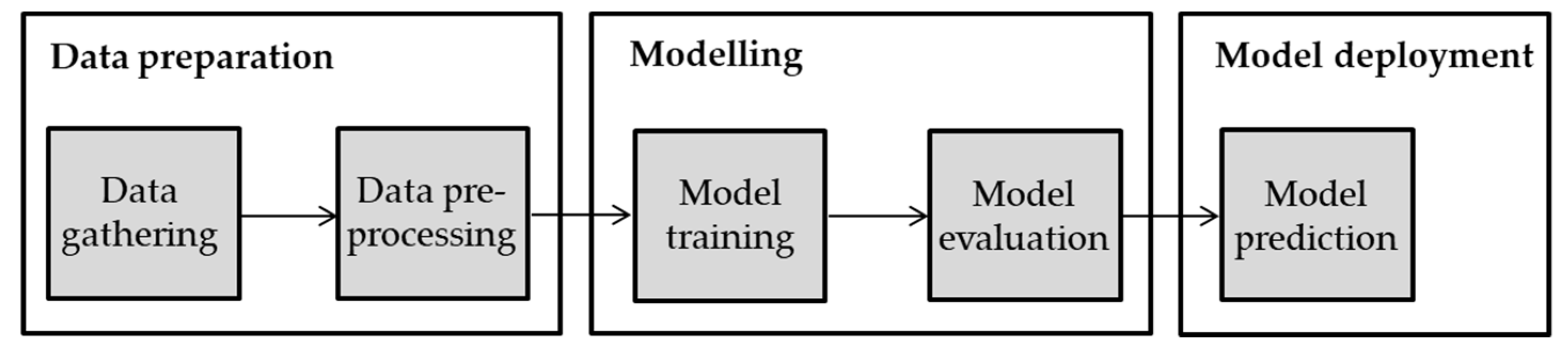
As introduced before, building stock decarbonisation is a fundamental component of the strategies to limit the impact of climate change. Buildings for education such as kindergartens, schools and universities display many similar design, operation and maintenance features in most countries in EU. The two most notable similarities between these building types are their high energy consumption and their inclusion in an ageing building stock, where significant energy saving measures are only rarely implemented due to decision-makers’ lack of knowledge regarding the effectiveness of potential energy saving measures [21], which require substantial investment and planning capacity. Beside energy demand, indoor air quality (IAQ) represents another important issue. In fact, even though the indoor environmental quality of a school has a strong influence on the health and productivity of students and teachers, poor indoor air quality has been reported in many cases in the published literature, even in newly constructed school buildings. The interplay between energy efficiency and indoor air quality is therefore a key issue for education buildings [22] and efficiency measures should address both aspects coherently, with an appropriate consideration of the trade-off between comfort, cost and environmental impact. More in general the sustainable long-term management of building stock requires multiple layers of information regarding its state (e.g., size and composition, etc.), dynamics (e.g., rate of new construction, refurbishment, demolition, etc.) and performance (e.g., energy and indoor air quality, etc.).

As a result, the use of data analytics, which refers to the process of examining datasets in order to draw conclusions about the information contained within them, is necessary to understand the temporal evolution of the stock considered [23] and digitalization appears as a crucial pre-requisite to perform these analytical processes efficiently and in a cost-effective way. As anticipated, investments are needed to increase the level of efficiency of the building stock as well as to increase its level of digitalization, but these investments can contribute to the economic recovery [5,24] in the post-pandemic period, as well as to the more ambitious (and long-term oriented) targets of net zero emissions and circular economy for the built environment [6].

Clearly, investments in energy efficiency have to deliver an appropriate level of performance, quantifiable in terms of energy and cost savings, which are the key enablers for innovative business models [3] built upon smart energy services and technologies. The techno-economic impact of energy efficiency measures should be assessed using cost-optimal analysis [25], which allows for the evaluation of the trade-offs between energy performance (or related carbon emissions) and cost (even life cycle cost) for multiple technologies at the same time. The operational cost determined by energy consumption is one of the components of cost-optimal analysis (together with investment cost, replacement cost and maintenance) and we decided to use it in this research for the reasons that will be illustrated in Section 3 hereafter.

3. Methods

Following the arguments presented in Section 2, which described the background and motivations for this research, we decided to use energy services cost as a variable in our study because it is an essential component of cost-optimal analysis (together with investment cost and maintenance cost) [25] and may be available in digital format for relatively long periods of time due to accounting procedures (tracking of expenses). In fact, even at low resolution, (e.g., monthly data from utility bills), energy performance monitoring data are rarely available in digital format for long periods (i.e., multiple years). This clearly represents a limiting factor (i.e., lack of robust evidence regarding energy performance). For this reason, we use in our research digital records of expenses for energy services obtained by the local public administration and weather data (air temperature in particular), from a local weather station. The study’s goal is to test the applicability of the modelling approach proposed as a screening tool for understanding the impact of energy efficiency measures and monitor energy related costs. The modelling approach can be seen as an extension of other regression-based approached for energy monitoring and Measurement and Verification (M & V), reviewed in recent literature [16,17]. While not as accurate and reliable as techniques for M & V [20,26,27], this regression-based approach can be nonetheless an inexpensive tool to track performance in time using cost data that are normally available in a digital format (e.g., for accounting purpose, as explained before) and may serve as a screening tool to assess the impact of efficiency measures across multiple buildings with similar characteristics when more contextual information is available. In this research, we present data in terms of energy services cost per unit of net floor area, to enable a comparison independent on the size of the building (but clearly dependent on its specific characteristics). Indeed, energy services cost is a “proxy” variable. A “proxy” variable is a variable that is not directly relevant in itself, but serves to replace an unobservable or immeasurable variable (in this case we assume energy consumption has not been recorded digitally). In order to be a good “proxy”, a variable must have a close correlation with the variable of interest. The cost of an energy service is determined by the amount of energy consumption and the unitary cost of energy. Therefore, it includes both dimensions (consumption and energy market dynamics) and it is subject to the temporal evolution of both. On the one hand, the amount of energy consumption, in particular for heating, cooling and ventilation services in buildings is highly influenced by weather conditions and the main independent variable for weather normalization is outdoor air temperature [28]. On the other hand, the unitary cost of energy depends on energy market dynamics and characteristics of energy service contracts.

The regression model proposed is substantially similar to the standardized ones described in ASHRAE 14:2014 [20] and ISO 50006:2014 [29] for energy monitoring. A continuous monitoring process in the long-term (i.e., across multiple years) determines the possibility to evaluate robustly the change in performance determined by efficiency measures and, in turn, could enable multiple feedback loops and could stimulate the continuous improvement process depicted in energy management standards such as ISO 50001:2018 [30].

From a technical standpoint, the model is a variable base degree-days one, proposed initially from Kissock et al. [31], which has been evolving steadily in time with the introduction of algorithmic techniques for the selection of base temperatures [32], up to the explicit solution for the three parameters case (heating and base load, as in this study). The definition of degree-days is itself part of international standards [33], even though the a-priori definition of a fixed base temperature (i.e., calculation of degree-days with a temperature established a priori [34]) is not correct when addressing individual buildings instead of groups of buildings (for which an average base temperature could be sufficient to perform weather normalization), as illustrated for example by Meng and Murshed [35]. Overall, recent technological advances in M & V, leading to M & V 2.0 [36], are yielding promising results that could be applied to the analysis of building performance at multiple levels and scales, including a physical interpretation of the regression coefficients [18], which can be employed also in the calibration [37] of detailed energy models [38]. Better models can aid in addressing the primary goals of efficiency and achieving stringent decarbonisation targets [1].

The different phases of the research and modelling workflow are reported in Figure 1. The data collection phase entails the acquisition of data from previous studies on the buildings under consideration, as well as the acquisition of digital records of public administration expenses for energy services for the buildings. The weather data for the corresponding period were then collected by a local weather station and provided by Meteonetwork, as mentioned in the acknowledgements. Following that, in the data pre-processing phase, we calculated the cost per unit of net floor area to improve cross-building comparability, and we defined the base temperature for calculating variable-base heating degree days (VB-HDD), using the method described in ISO 15927-6:2007 [33]. Following that, the regression models (for various buildings) were trained, and their performance was assessed using R² and adjusted R² (indicated in ISO 50006:2014 [33] as indicators for baseline energy models), as well as Mean Absolute Deviation (MAD) and Root Mean Square Error (RMSE) [39] to understand their goodness of fit. Finally, the trained regression models were used with a reference weather dataset (input) to predict heating service cost (output) in reference conditions.

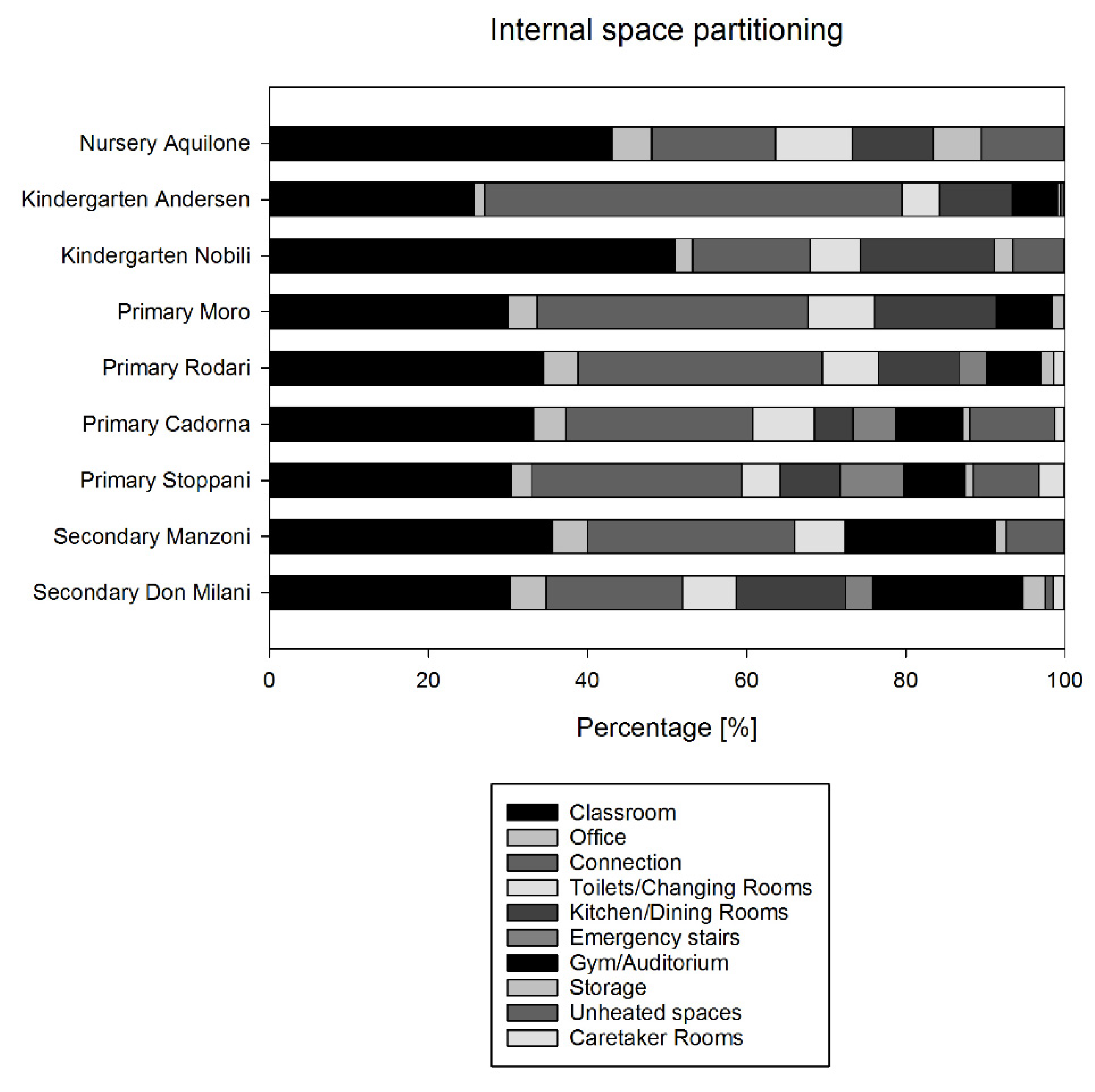
4. Case Study Description

The case study consists of nine public schools in Seregno, Province of Monza-Brianza, in Northern Italy. All of these buildings were monitored for six years (2009–2014) and two of them were monitored for an additional two years (2015–2016) after some renovation measures were implemented. In

Table 1. Building characteristics summary.

N°	School Name	Type of School	Total Net Floor Area (m2)	Floor Shape	Year of Construction	Renovation
1	Asilo Nido Aquilone	Nursery	867.2		1975	No
2	Scuola dell’Infanzia H.C. Andersen	Kindergarten	2116.4		1973	Yes, 1999, 2013/14
3	Scuola dell’Infanzia Nobili	Kindergarten	2049.6		1969	No
4	Istituto Comprensivo Aldo Moro	Primary	4487.2		1972	Yes, 2014/15
5	Istituto Comprensivo Gianni Rodari	Primary	4815.5		1974	No
6	Istituto Comprensivo Luigi Cadorna	Primary	6500.1		1920–1940	No
7	Istituto Comprensivo Antonio Stoppani	Primary	2325.0		1900–1920	No
8	Istituto Comprensivo Alessandro Manzoni	Secondary	4255.0		1970	No
9	Scuola Secondaria Don Milani	Secondary	6945.3		1987	No

, we present a summary of building characteristics, including the school name, type, total net floor area, floor shape, year of construction and renovation process. In Figure 1 we indicate the subdivision of space according to different functions (i.e., space partitioning).

The two buildings renovated are Andersen Kindergarten (number 2 in Table 1) and Moro School (number 4 in Table 1). The efficiency measures applied were, respectively, glazing system substitution for Andersen Kindergarten and heating system refurbishment for Moro School. In the first building, the effect of efficiency measures was already visible during year 2014, while in the second building the renovations was more profound and the building was not operated during year 2015 and reopened during 2016. As anticipated, we can analyse the partitioning of internal spaces based on the reported functions in Figure 2 to gain a better understanding of the characteristics of all the buildings considered in this study. All the buildings allocate similar percentages for similar functions, with the exception of Aquilone Nursery and Nobili Kindergarten, which have more space for classrooms.

As explained in Section 3, the goal of this paper is to adapt a well-developed regression-based approach used for energy data analysis to another “proxy” variable, heating service cost. By comparing the data in a weather-normalized manner, we can determine the impact of efficiency measures on energy services costs per unit of net floor area before and after renovation. In our analysis, we concentrate on the cost of heating service, which is the highest cost and has a significant temperature dependence, implying the necessity of weather normalisation of data. The use of a “proxy” variable is considered because it could allow long-term analysis of energy performance even when energy consumption data have not been recorded digitally for a long period of time, which is what happens in many cases, especially in old buildings. While energy data may not be directly available, utility bill payments may be available in digital form, at least in recent years, due to accounting procedures. As a result, where these data are available in digital form, this represents an opportunity for building stock digitalization, both in the public and private sectors. Therefore, in this research we use monthly utility billing data, made available in digital format by the local public administration, and weather data, recorded from a local weather monitoring station. As anticipated in Section 3, the model proposed is similar to the ones used reported in ASHRAE 14:2014 [20] and in particular to the three parameters model, focused on heating and baseline energy demand.

As anticipated in Section 3 and in Figure 1, we consider monthly heating service cost per unit of floor area, expressed in €/m², as the dependent variable and variable base heating degree-days (VB-HDD) as the independent variable to enable a meaningful comparison independent on the size of each individual building. The calculation of VB-HDD is performed after determining a base temperature specific to each building, as discussed in greater detail in the following section, using the method described in ISO 15927-6:2007 [33]. The developed regression models are then used to compare performance with a reference design weather data file [40] for which the VB-HDD variable was calculated with the same building specific base temperature mentioned before.

5. Results and Discussion

As reported in the introduction, the two fundamental questions are whether it is possible to use variable-base degree-days regression models for the long-term monitoring of energy services cost and what is the goodness of fit that they can achieve using monthly utility billing data, frequently available in digital format. First of all, we report the ranges of cost for heating and electricity services for all the buildings, from year 1 to year 6 (2009–2014). The cost of heating service is much larger and generally much more variable (due to weather dependence) than the one for electricity as can be seen in Figure 3.

The data are then reported in

Table 2. Yearly costs of heating service per unit of net floor area for all the buildings.

School Name and Type	Monitoring Years						Range of Data
	2009	2010	2011	2012	2013	2014	Min	Avg	Max
	€/m2	€/m2	€/m2	€/m2	€/m2	€/m2	€/m2	€/m2	€/m2
Nursery Aquilone	25.8	25.8	26.1	34.5	41.4	35.4	25.8	31.5	41.4
Kindergarten Andersen	10.4	13.9	12.5	12.6	13.2	8.7	8.7	11.9	13.9
Kindergarten Nobili	15.9	15.5	12.2	15.0	25.5	20.9	12.2	17.5	25.5
Primary Moro	10.7	12.0	13.2	18.0	17.5	12.9	10.7	14.1	18.0
Primary Cadorna	8.8	13.2	8.3	19.0	19.7	14.0	8.3	13.8	19.7
Primary Rodari	12.6	13.2	12.4	16.3	16.1	10.3	10.3	13.5	16.3
Primary Stoppani	12.3	9.3	11.4	14.3	16.9	12.3	9.3	12.8	16.9
Secondary Manzoni	11.4	11.6	8.5	13.0	11.8	10.9	8.5	11.2	13.0
Secondary Don Milani	13.9	17.2	12.1	15.5	20.1	15.2	12.1	15.7	20.1

and

Table 3. Yearly costs of electricity service per unit of net floor area for all the buildings.

School Name and Type	Monitoring Years						Range of Data
	2009	2010	2011	2012	2013	2014	Min	Avg	Max
	€/m2	€/m2	€/m2	€/m2	€/m2	€/m2	€/m2	€/m2	€/m2
Nursery Aquilone	6.2	5.8	5.7	6.6	6.7	6.8	5.7	6.3	6.8
Kindergarten Andersen	2.1	3.1	2.5	2.9	3.3	3.4	2.1	2.9	3.4
Kindergarten Nobili	7.0	7.0	7.4	8.9	9.1	9.4	7.0	8.1	9.4
Primary Moro	5.2	4.6	4.7	5.2	6.0	6.2	4.6	5.3	6.2
Primary Cadorna	4.4	4.8	5.0	5.1	5.8	5.3	4.4	5.1	5.8
Primary Rodari	4.4	4.2	4.5	5.3	5.6	5.7	4.2	5.0	5.7
Primary Stoppani	4.5	4.0	4.4	4.4	4.7	4.2	4.0	4.4	4.7
Secondary Manzoni	2.6	2.1	1.8	2.1	2.3	2.0	1.8	2.1	2.6
Secondary Don Milani	3.3	3.5	3.2	4.0	4.3	4.2	3.2	3.8	4.3

, respectively, for heating service and electricity service, with summary statistics minimum, average, maximum.

In the next Section we focus on the two buildings that have been renovated, Andersen Kindergarten and Moro School, developing a more in-depth analysis.

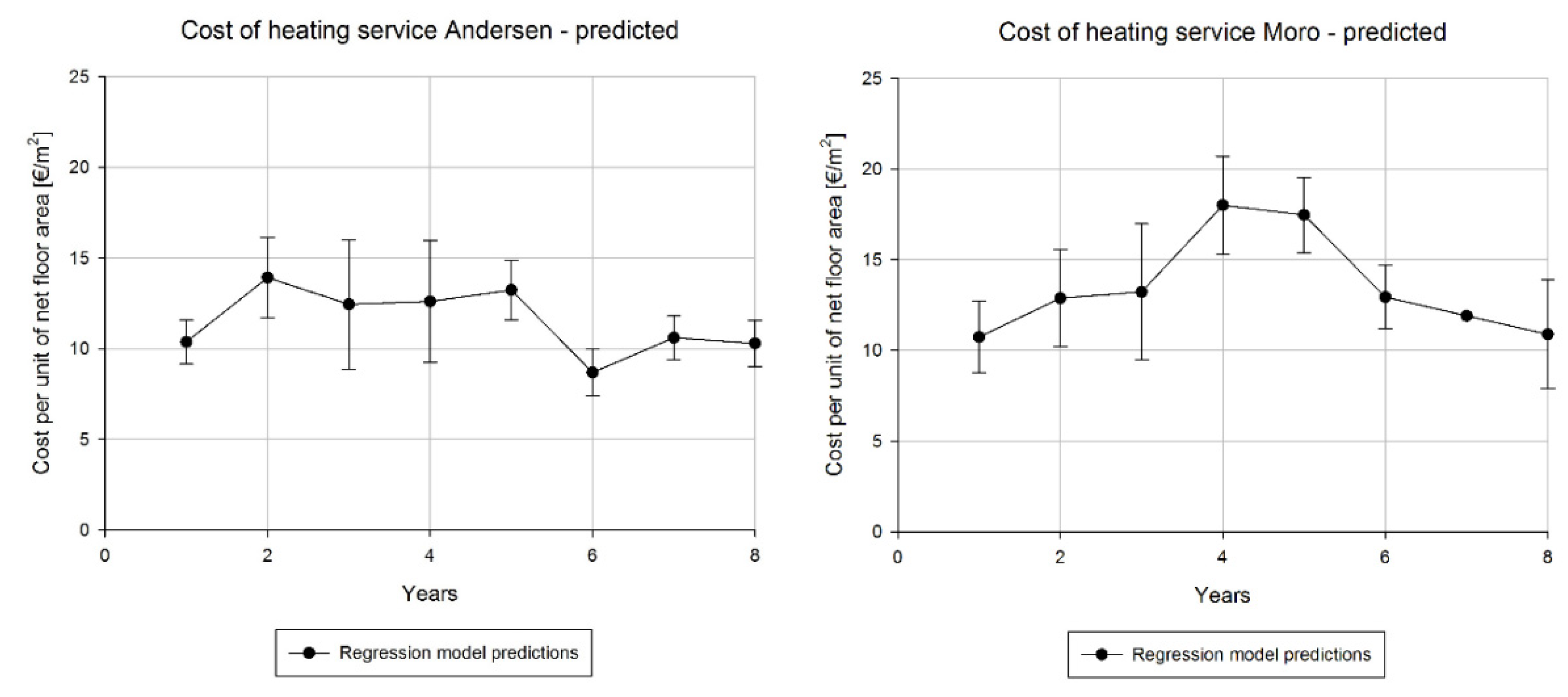
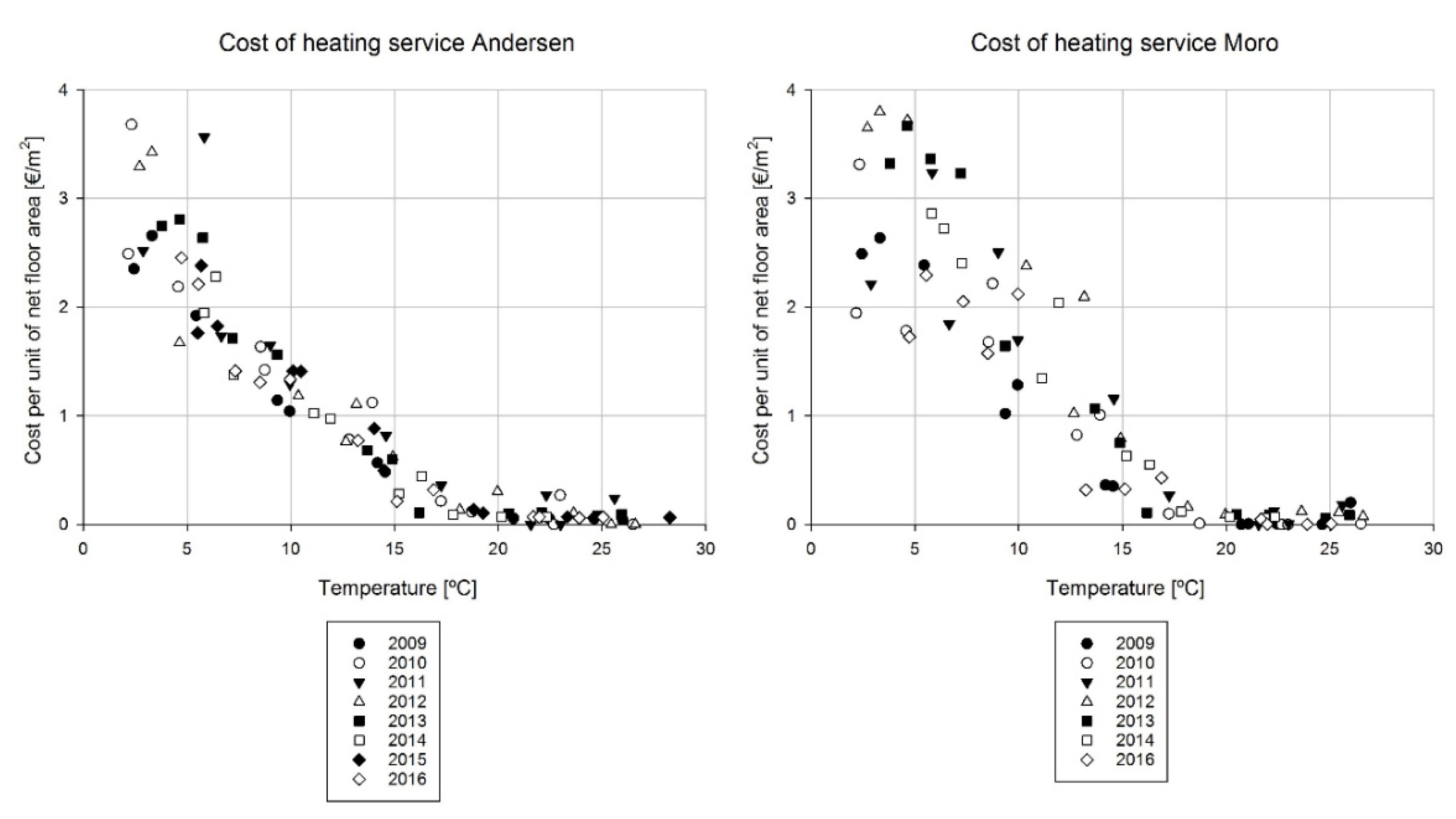
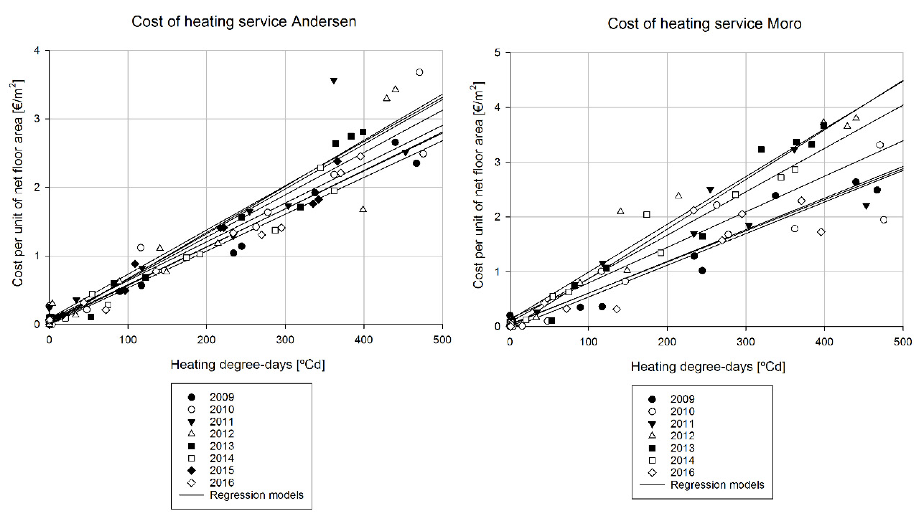
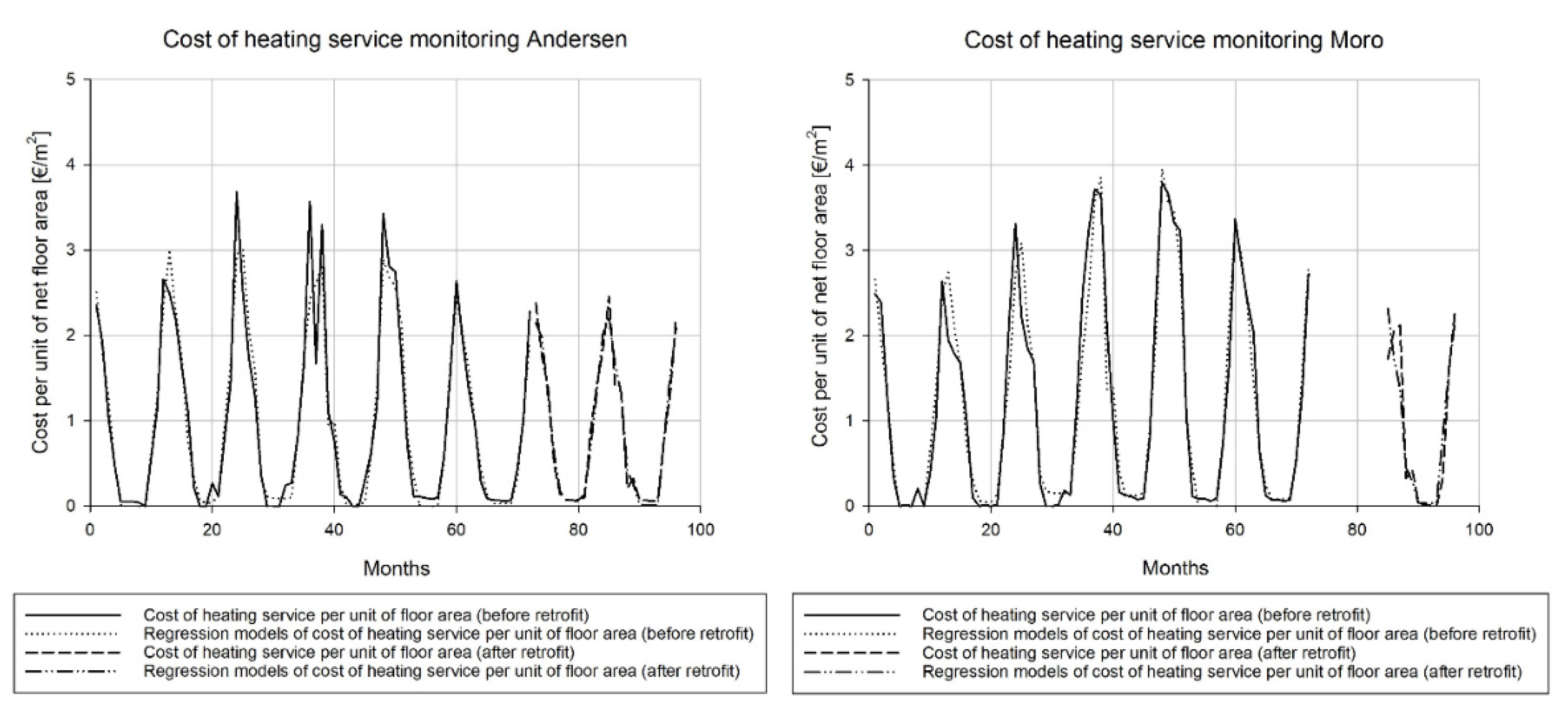
5.1. Analysis of Heating Service Cost before and after Renovation for Andersen Kindergarten and Moro School

Hereafter, we present the application of the regression-based approach introduced in Section 3 to the two renovated buildings, Andersen Kindergarten and Moro School. The main steps of the analysis process are depicted below. In the first phase, we established the base temperature to be used when calculating variable base heating degree-days (VB-HDD) by plotting heating service cost (per unit of net floor area) with respect to temperature. This is depicted graphically in Figure 3 and will be explained more in detail later. After determining the base temperature, the VB-HDD was calculated using the method described in ISO 15927-6:2007 [33]. The third step was the training and evaluation of regression models. The fourth and final step was to use the regression models with a reference design weather data file to allow for a weather-normalized comparison of heating service cost. While the original regression method was the one proposed in ASHRAE 14:2014 [20], which provides rigorous rules and thresholds for the acceptability of models using statistical indicators such as Normalized Mean Bias Error (NMBE) and Coefficient of Variation of Root Mean Square Error (CV(RMSE)), in this case we consider more basic statistical indicators such as R², adjusted R². Mean Absolute Deviation (MAD) and Root Mean Square Error (RMSE) [39]. R² and adjusted R² are indicated in ISO 50006:2014 [29] as indicators to understand the goodness of fit of energy models. These two statistical indicators range from 0 (no correlation) to 100% (perfect fit to a linear model).

In Figure 4, we plot the cost of heating service per unit of floor area on a monthly basis (y-axis) for both Andersen Kindergarten and Moro School, in relation to the monthly average outdoor air temperature (x-axis). In this manner, we can graphically identify the correlation between the two variables as well as the appropriate model to use. We can clearly see that the shape in this case is the one of a three parameter model, as defined in ASHRAE 14:2014 [20], i.e., a piecewise linear regression with a constant term and a temperature dependent term that starts below the base temperature, which in both buildings is approximately 17.5 °C. The base temperature is essentially the average outdoor temperature that corresponds to a heating demand equal to zero. When the temperature is lower than the base temperature, we can have a base load determined by hot water demand for sanitary use. The base temperature depends on the thermal characteristics of the building, the use of spaces, the operational strategies, and the behaviour of the occupants. As a result, it may differ from building to building, as shown in recent research [35], and must be considered as the first step in developing an appropriate regression model for the specific building. The piecewise linear pattern is clear for Andersen Kindergarten while data are more scattered for Moro School. However, in both cases the base temperature is approximately 17.5 °C.

Variable-base heating degree-days (VB-HDD) were computed after selecting 17.5 °C as the base temperature, and the same data in Figure 4 were reported in Figure 5 as a function of VB-HDD. It is clear in this case how multiple linear models can be used to fit the behaviour year after year. We created one model for each year because we didn’t know a priori the evolution of the unitary energy cost for the service (i.e., the variation of the unitary cost year on year) and wanted to test it as a top-down approach to identify anomalies in the cost’s evolution.

Following the correlation analysis in Figure 4, we can see how for Moro School data have a larger spread than for Andersen Kindergarten. This is reflected in a much greater year-to-year variation in the slopes of regression models. In turn, this indicates an anomaly because, after removing the temperature dependence (VB-HDD), the slope variability can be determined by tariff evolution, operational changes or performance degradation, which should have a reasonably a smaller magnitude (as in Andersen Kindergarten for example) compared to what we see in the case of Moro School in Figure 5 on the right. In this case, the rapid variation of slope was determined by a performance degradation of the heating system, which has been renovated then in 2014/15.

Hereafter we present the numerical results of the regression analysis for both buildings, respectively in

Table 4. Results of VB-HDD regression models—Andersen Kindergarten.

N°	Year	Weather	Economic Indicators		Statistical Indicators
		VB-HDD	Yearly Cost Measured	Yearly Cost Predicted	R2	Adj-R2	MAD	RMSE
		°Cd	€/m2	€/m2	%	%	€/m2	€/m2
1	2009	1936	10.4	10.4 ± 1.2	97.9	97.7	0.10	0.13
2	2010	2178	13.9	13.9 ± 2.2	92.8	92.1	0.22	0.30
3	2011	1766	12.5	12.5 ± 3.6	87.4	86.1	0.25	0.39
4	2012	1898	12.6	12.6 ± 3.4	89.7	88.7	0.26	0.37
5	2013	1973	13.2	13.2 ± 1.6	97.2	96.9	0.15	0.18
6	2014	1510	8.7	8.7 ± 1.3	96.6	96.3	0.10	0.14
7	2015	1717	10.6	10.6 ± 1.2	97.3	97.1	0.10	0.13
8	2016	1818	10.3	10.3 ± 1.3	97.2	96.9	0.11	0.14

for Andersen Kindergarten and in

Table 5. Results of VB-HDD regression models—Moro School.

N°	Year	Weather	Economic Indicators		Statistical Indicators
		VB-HDD	Yearly Cost Measured	Yearly Cost Predicted	R2	Adj-R2	MAD	RMSE
		°Cd	€/m2	€/m2	%	%	€/m2	€/m2
1	2009	1936	10.7	10.7 ± 2.0	95.5	95.0	0.16	0.21
2	2010	2178	12.9	12.9 ± 2.7	87.3	86.0	0.27	0.38
3	2011	1766	13.2	13.2 ± 3.8	86.3	84.9	0.29	0.41
4	2012	1898	18.0	18.0 ± 2.7	96.1	95.7	0.21	0.29
5	2013	1973	17.5	17.5 ± 2.1	97.5	97.3	0.17	0.23
6	2014	1510	12.9	12.9 ± 1.8	96.9	96.6	0.11	0.19
7	2015	1717	-	-	-	-	-	-
8	2016	1818	10.9	10.9 ± 3.0	86.9	85.6	0.22	0.33

for Moro School. The goodness of fit achieved by the models in the first case (Andersen Kindergarten) is high (R² in the range 87.4–97.9%, Adj-R² 88.7–97.7%) and the uncertainty in the prediction of cost on a yearly base is relatively small, as expected due to the relative modest spread of data.

On the other hand, in the second building (Moro School) the goodness of fit achieved by the models (R² in the range 86.3–97.5%, Adj-R² 84.9–97.3%) is high as well, but the uncertainty in the prediction of cost on a yearly base is much larger, despite having similar values, as expected due to the larger spread of data already highlighted in the previous steps of the analysis. The results of the regression predictions are then plotted in time (monthly intervals) in Figure 6 for the entire monitoring period (96 months) for both buildings; the Moro building was not in operation in 2015.

We can see how, despite their simplicity, the models can approximate the temporal pattern quite well, with only a few points where the difference (measured-predicted) is significant. To go deeper into the analysis from a time series perspective, we would obviously need energy consumption and unitary cost of energy as separate variables (the selected “proxy” variable is the product of the two, as discussed in Section 3), but this is not part of this research, which aims to highlight the possibility of using this method as a screening tool. Nonetheless, we can try to identify if there is a recurrent pattern in the deviations between measured data and model predictions for monthly costs of heating service per unit of net floor area, which could depend on the utility billing method.

As can be seen in Figure 7 there is a quite large oscillation of the deviations, but we cannot identify a clear pattern in them. After that, we summed up the monthly values of regression predictions to obtain the yearly value (with its confidence interval) and the results are reported in Figure 8, again for both buildings.

The cost for 2015 for Moro School is reported as a linear interpolation due to the missing data point and we can see how the cost increase is particularly relevant between year 3 and 4 (2011–2012), probably determined by a rapid performance degradation and operational changes. The results identified in Figure 8 are still dependent on the specific weather year on year but our goal is identifying the actual evolution by projecting the cost using a reference design weather data file [40], for which VB-HDD has been calculated, using 17.5 °C as base temperature, for the reasons specified before. With this weather data file, we obtain 2147 °Cd and the corresponding results are reported (with their confidence interval) in Figure 9, highlighting a consistent increase in cost for Moro School from year 2 (2010) up to 4 (2012).

Finally, we employ the same method as in Figure 9 to determine the cost savings achieved by efficiency measures, employing 2147 °Cd (reference year) and 2013 for Andersen and 2014 for Moro School. The savings percentages achieved, 16% and 30%, are indicated in

Table 6. Identification of cost savings using VB-HDD regression models for typical design year—Andersen Kindergarten and Moro School.

School Name	VB-HDD	Before Retrofit— Reference Year	Before Retrofit— Cost	After Retrofit— Cost	Relative Variation— Savings
	°Cd		€/m2	€/m2	%
Andersen	2147	2013	14.4 ± 1.7	12.1 ± 1.3	−16%
Moro	2147	2014	18.0 ± 1.8	12.8 ± 3.1	−30%

and are plausible for the renovation measures implemented, namely the replacement of the glazing system for Andersen Kindergarten and the refurbishment of the heating system for Moro School. This confirms the suitability of the approach as a screening tool.

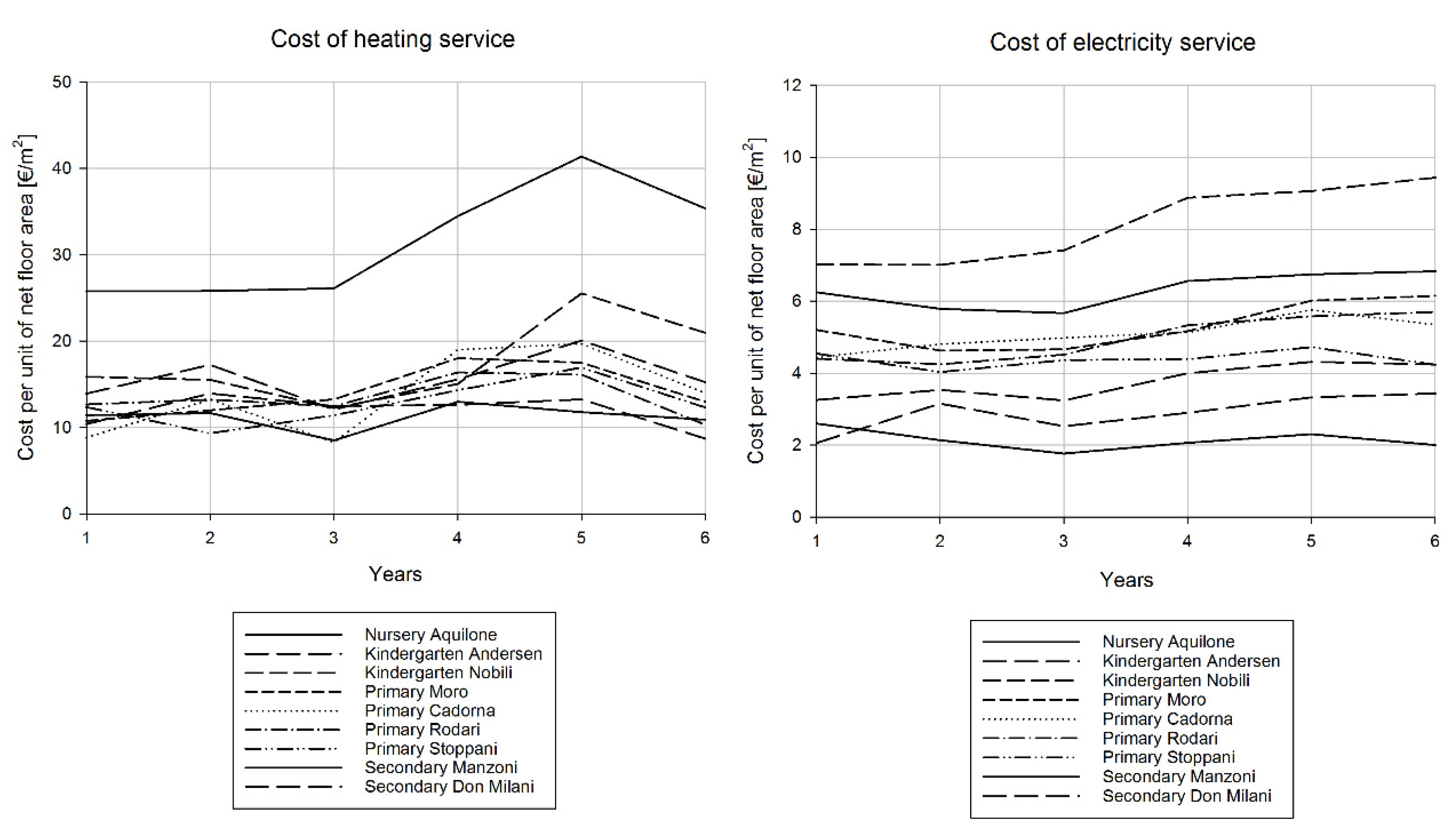
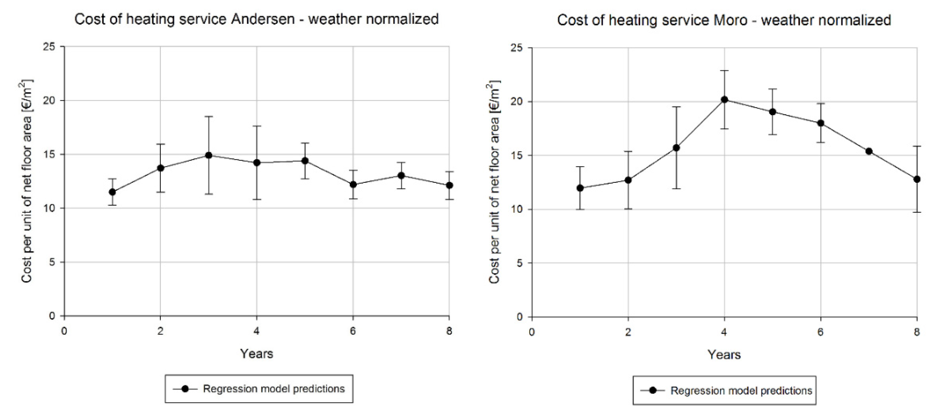
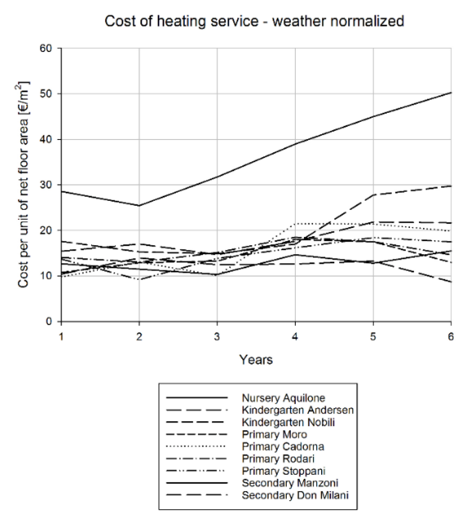
5.2. Comparison of Heating Service Cost after Weather Normalisation for All the Buildings in This Study

In this Section we use the same methodological approach employed before for the weather normalization of heating service cost for Andersen Kindergarten and Moro (presented in Section 5.1), but we apply it to the all the building considered in the study for the first 6 years of monitoring (2009–2014).

We present the data in Figure 10, similarly to Figure 3 and Table 2 at the beginning of this section, but we compute them with the VB-HDD of the reference year chosen for comparison [40]. The corresponding data are reported in

Table 7. Yearly costs of heating services per unit of net floor area—Weather normalized model predictions for all buildings.

School Name and Type	Monitoring Years						Range of Data
	2009	2010	2011	2012	2013	2014	Min	Avg	Max
	€/m2	€/m2	€/m2	€/m2	€/m2	€/m2	€/m2	€/m2	€/m2
Nursery Aquilone	28.6	25.4	31.7	39.0	45.0	50.3	25.4	36.7	50.3
Kindergarten Andersen	10.4	13.9	12.5	12.6	13.2	8.7	8.7	11.9	13.9
Kindergarten Nobili	17.6	15.3	14.9	17.0	27.8	29.8	14.9	20.4	29.8
Primary Moro	10.7	12.9	13.2	18.0	17.5	12.9	10.7	14.2	18.0
Primary Cadorna	9.8	13.0	10.0	21.5	21.4	19.8	9.8	15.9	21.5
Primary Rodari	14.0	13.0	15.1	18.5	17.5	14.6	13.0	15.5	18.5
Primary Stoppani	13.7	9.2	13.8	16.2	18.4	17.5	9.2	14.8	18.4
Secondary Manzoni	12.7	11.5	10.3	14.7	12.8	15.5	10.3	12.9	15.5
Secondary Don Milani	15.4	17.0	14.7	17.6	21.8	21.6	14.7	18.0	21.8

. We can see that there is a moderate shift in costs between year 3 (2011) and 4 (2012) for most of the buildings, but the most evident anomalies are represented by Aquilone Nursery and Nobili Kindergarten which show a strong increasing trend in cost of heating service and should be considered for more in-depth analysis.

Overall, the modelling process described here allows for the normalisation of energy cost data as well as the detection of anomalies and changes of relevant entity. As anticipated, it could be used for a low-cost screening analysis when billing and temperature data are easily accessible in digital format, with some potential extensions discussed in the following section.

5.3. Limitations and Further Research

The limitations of this research have been partially anticipated in Section 3 and they reside in the fact that we are using a consolidated technique (regression using variable-base degree-days) on a “proxy” variable, heating service cost, which depends on both the amount of energy consumption for heating (influenced by weather as well as other factors) and the unitary cost of energy (influenced by energy market dynamics). The method presented cannot be as accurate as the ones for M & V from which it has been derived (due to the multiple underlying dynamic and potential errors). Furthermore, as described in Section 5.1 and indicated in Figure 3, the selection of the base temperature (i.e., the change-point for the piecewise linear regression) has been determined by means of graphical analysis. This step can be automated further, as Paulus et al. [32] discuss, and the search range for base temperatures can be informed by an analysis of building characteristics [35]. Nonetheless, even in absence of long-term energy monitoring data, when energy services costs are available in digital format for accounting purpose, this modelling approach can be applied as a simple screening tool effectively and its application can be easily automated, exploiting also the interpretability of the regression modelling techniques [16] to identify the impact of building characteristics on base temperature and slope. Overall, our study aims to help in the process of building stock digitalization that is a key step in the process of meeting decarbonisation targets and can be framed within an area of research that uses the fundamentals of building energy calibration techniques [37] to create data-driven workflows that can be applied at different stages of the building life cycle, e.g., early design stage optimization [41], automated identification of best-fitting models [42] and operational patterns [43] and linking with top-down statistical analysis [44]. In this sense, different types of models, if properly designed for interoperability and combined into systems [45] can determined a radical contribution to the digital transformation of the built environment, becoming “digital twins”. A “digital twin” is a computer-generated representation of a physical object, process, or service (i.e., a digital replica) that can overcome the limitations of the simulation-based approaches normally used in engineering. While simulations and “digital twins” are both virtual representations of objects, digital twins can verify how a physical object, process or service performs in real time and in real world conditions, providing a continuous feedback loop (and consequently continuous improvements). Furthermore, when interpretable data-driven techniques are employed [16] it is becomes possible to combine human and machine intelligence in a virtuous circle (human-in-the-loop approach), whose fundamental goals can be that of accelerating the transition towards a net zero carbon society.

6. Conclusions

The essential goals of this research work were fundamentally two. The first one was testing the applicability of regression-based techniques, originally developed for Measurement & Verification (M & V), to energy services cost analytics. The second one was to normalize energy services cost with respect to weather conditions and highlight the actual reduction determined by energy efficiency measures, with an approach resembling the one used for energy consumption in M & V, but applied to a “proxy” variable, in this case heating service cost. Overall, we highlighted the fact that a regression-based approach can work reasonably well as a screening method even with limited information such as monthly data, making it suitable for quick and inexpensive performance assessment (potentially on a large-scale base, due to its scalability and possibility of automation), using data records of utility bills and basic weather data. Additionally, multiple directions for further research in this area have been indicated, highlighting the fact that different data-driven models can work a system, if properly conceived. The more relevant directions for further research are related to model automation and integration with other techniques, to complement them. The first aspect is related to the automation of base point temperature selection in regression-based models and subsequently to the calculation of variable-base degree-days. As already discussed in the paper, base temperature depends on several building characteristics and can have a certain variability; the ability to define it in an automated way for multiple building typologies, can greatly enhance the scalability of the approach. The second aspect is related to the integration of this approach with other regression-based approaches for M & V; in this case, measured energy services cost could be helpful as a benchmark which involves both energy tariffs and energy consumption in an integrated way, together with contextual information. As a conclusion, the possibility to combine multiple analytical techniques, from top-down to bottom-up, can highly increase the reliability of estimates in techno-economic assessment, which is crucial for the deployment of innovative business models and technologies in the built environment in present state and in future perspective.

References

1. Norton, B.; Gillett, W.B.; Koninx, F. Decarbonising Buildings in Europe: A Briefing Paper. Proc. Inst. Civ. Eng. Energy 2021, 174, 147–155. [Google Scholar] [CrossRef]
2. Esser, A.; Dunne, A.; Meeusen, T.; Quaschning, S.; Denis, W.; Hermelink, A.; Schimschar, S.; Offermann, M.; John, A.; Reiser, M.; et al. Comprehensive Study of Building Energy Renovation Activities and the Uptake of Nearly Zero-Energy Buildings in the EU Final Report; Publications Office of the European Union: Luxembourg, 2019. [Google Scholar]
3. Manfren, M.; Nastasi, B.; Tronchin, L.; Groppi, D.; Garcia, D.A. Techno-economic analysis and energy modelling as a key enablers for smart energy services and technologies in buildings. Renew. Sustain. Energy Rev. 2021, 150, 111490. [Google Scholar] [CrossRef]
4. Sibilla, M.; Manfren, M. Envisioning Building-as-Energy-Service in the European context. From a literature review to a conceptual framework. Archit. Eng. Des. Manag. 2021, 1–26. [Google Scholar] [CrossRef]
5. Unsworth, S.; Andres, P.; Cecchinato, G.; Mealy, P.; Taylor, C.; Valero, A. Jobs for a Strong and Sustainable Recovery from COVID-19; Centre for Economic Performance, London School of Economics and Political Science: London, UK, 2020. [Google Scholar]
6. McKinsey. Growth Within: A Circular Economy Vision for a Competitive Europe; McKinsey Center for Business and Environment: New York, NY, USA, 2014. [Google Scholar]
7. Xing, Y.; Hewitt, N.; Griffiths, P. Zero carbon buildings refurbishment––A Hierarchical pathway. Renew. Sustain. Energy Rev. 2011, 15, 3229–3236. [Google Scholar] [CrossRef]
8. Castro, S.S.; Suárez López, M.J.; Menéndez, D.G.; Marigorta, E.B. Decision matrix methodology for retrofitting techniques of existing buildings. J. Clean. Prod. 2019, 240, 118153. [Google Scholar] [CrossRef]
9. The Energy Benchmarking Tool—CIBSE. Available online: https://www.cibse.org/knowledge/digital-tools/the-energy-benchmarking-tool-(beta-version) (accessed on 23 November 2021).
10. Robertson, C.; Mumovic, D.; Hong, S.M. Crowd-sourced building intelligence: The potential to go beyond existing benchmarks for effective insight, feedback and targeting. Intell. Build. Int. 2015, 7, 147–160. [Google Scholar] [CrossRef]
11. Pfenninger, S.; DeCarolis, J.; Hirth, L.; Quoilin, S.; Staffell, I. The importance of open data and software: Is energy research lagging behind? Energy Policy 2017, 101, 211–215. [Google Scholar] [CrossRef]
12. Burman, E.; Hong, S.-M.; Paterson, G.; Kimpian, J.; Mumovic, D. A comparative study of benchmarking approaches for non-domestic buildings: Part 2—Bottom-up approach. Int. J. Sustain. Built Environ. 2014, 3, 247–261. [Google Scholar] [CrossRef] [Green Version]
13. Hong, S.-M.; Paterson, G.; Burman, E.; Steadman, P.; Mumovic, D. A comparative study of benchmarking approaches for non-domestic buildings: Part 1—Top-down approach. Int. J. Sustain. Built Environ. 2013, 2, 119–130. [Google Scholar] [CrossRef] [Green Version]
14. ISO/IEC. TR 29119-11:2020(en) Software and Systems Engineering—Software Testing—Part 11: Guidelines on the Testing of AI-Based Systems; ISO: Geneva, Switzerland, 2020. [Google Scholar]
15. Lipton, Z.C. The Mythos of Model Interpretability: In machine learning, the concept of interpretability is both important and slippery. Queue 2018, 16, 31–57. [Google Scholar] [CrossRef]
16. Manfren, M.; Sibilla, M.; Tronchin, L. Energy Modelling and Analytics in the Built Environment—A Review of Their Role for Energy Transitions in the Construction Sector. Energies 2021, 14, 679. [Google Scholar] [CrossRef]
17. Manfren, M.; Nastasi, B.; Tronchin, L. Linking Design and Operation Phase Energy Performance Analysis Through Regression-Based Approaches. Front. Energy Res. 2020, 8, 288. [Google Scholar] [CrossRef]
18. Tronchin, L.; Manfren, M.; Nastasi, B. Energy analytics for supporting built environment decarbonisation. Energy Procedia 2019, 157, 1486–1493. [Google Scholar] [CrossRef]
19. ISO. 16346:2013 Energy Performance of Buildings—Assessment of Overall Energy Performance; ISO: Geneva, Switzerland, 2013. [Google Scholar]
20. ASHRAE. ASHRAE Guideline 14-2014: Measurement of Energy, Demand, and Water Savings; American Society of Heating, Refrigerating and Air-Conditioning Engineers: Atlanta, GA, USA, 2014. [Google Scholar]
21. Erhorn, H.; Mroz, T.; Mørck, O.; Schmidt, F.; Schoff, L.; Thomsen, K.E. The Energy Concept Adviser—A tool to improve energy efficiency in educational buildings. Energy Build. 2008, 40, 419–428. [Google Scholar] [CrossRef]
22. Dascalaki, E.G.; Sermpetzoglou, V.G. Energy performance and indoor environmental quality in Hellenic schools. Energy Build. 2011, 43, 718–727. [Google Scholar] [CrossRef]
23. Kohler, N.; Yang, W. Long-term management of building stocks. Build. Res. Inf. 2007, 35, 351–362. [Google Scholar] [CrossRef] [Green Version]
24. OECD. Making the Green Recovery Work for Jobs, Income and Growth. Available online: https://www.oecd.org/coronavirus/policy-responses/making-the-green-recovery-work-for-jobs-income-and-growth-a505f3e7/ (accessed on 23 November 2021).
25. Ferrara, M.; Monetti, V.; Fabrizio, E. Cost-Optimal Analysis for Nearly Zero Energy Buildings Design and Optimization: A Critical Review. Energies 2018, 11, 1478. [Google Scholar] [CrossRef] [Green Version]
26. EVO IPMVP New Construction Subcommittee. International Performance Measurement & Verification Protocol: Concepts and Option for Determining Energy Savings in New Construction; Efficiency Valuation Organization (EVO): Washington, DC, USA, 2003; Volume 3. [Google Scholar]
27. FEMP. Federal Energy Management Program, M&V Guidelines: Measurement and Verification for Federal Energy Projects Version 3.0; U.S. Department of Energy Federal Energy Management Program: Washington, DC, USA, 2008. [Google Scholar]
28. Fazeli, R.; Ruth, M.; Davidsdottir, B. Temperature response functions for residential energy demand—A review of models. Urban Clim. 2016, 15, 45–59. [Google Scholar] [CrossRef]
29. ISO. 50006:2014 Energy Management Systems—Measuring Energy Performance Using Energy Baselines (EnB) and Energy Performance Indicators (EnPI)—General Principles and Guidance; ISO: Geneva, Switzerland, 2014. [Google Scholar]
30. ISO. 50001:2018 Energy Management Systems—Requirements with Guidance for Use; ISO: Geneva, Switzerland, 2018. [Google Scholar]
31. Kissock, J.K.; Haberl, J.S.; Claridge, D.E. Inverse modeling toolkit: Numerical algorithms. ASHRAE Trans. 2003, 109, 425. [Google Scholar]
32. Paulus, M.T.; Claridge, D.E.; Culp, C. Algorithm for automating the selection of a temperature dependent change point model. Energy Build. 2015, 87, 95–104. [Google Scholar] [CrossRef]
33. ISO. 15927-6:2007 Hygrothermal Performance of Buildings—Calculation and Presentation of Climatic Data—Part 6: Accumulated Temperature Differences (Degree-Days); ISO: Geneva, Switzerland, 2007. [Google Scholar]
34. Azevedo, J.A.; Chapman, L.; Muller, C.L. Critique and suggested modifications of the degree days methodology to enable long-term electricity consumption assessments: A case study in Birmingham, UK. Meteorol. Appl. 2015, 22, 789–796. [Google Scholar] [CrossRef]
35. Meng, Q.; Mourshed, M. Degree-day based non-domestic building energy analytics and modelling should use building and type specific base temperatures. Energy Build. 2017, 155, 260–268. [Google Scholar] [CrossRef]
36. Granderson, J.; Fernandes, S. The state of advanced measurement and verification technology and industry application. Electr. J. 2017, 30, 8–16. [Google Scholar] [CrossRef] [Green Version]
37. Chong, A.; Gu, Y.; Jia, H. Calibrating building energy simulation models: A review of the basics to guide future work. Energy Build. 2021, 253, 111533. [Google Scholar] [CrossRef]
38. Fumo, N.; Torres, M.J.; Broomfield, K. A multiple regression approach for calibration of residential building energy models. J. Build. Eng. 2021, 43, 102874. [Google Scholar] [CrossRef]
39. Montgomery, D.C.; Peck, E.A.; Vining, G.G. Introduction to Linear Regression Analysis; John Wiley & Sons: Hoboken, NJ, USA, 2021. [Google Scholar]
40. UNI. 10349-1:2016 Riscaldamento e Raffrescamento Degli Edifici—Dati Climatici—Parte 1: Medie Mensili per la Valutazione Della Prestazione Termo-Energetica Dell’Edificio e Metodi per Ripartire L’Irradianza Solare Nella Frazione Diretta e Diffusa e per; UNI: Milan, Italy, 2016. [Google Scholar]
41. Kang, H.J. Development of an Nearly Zero Emission Building (nZEB) Life Cycle Cost Assessment Tool for Fast Decision Making in the Early Design Phase. Energies 2017, 10, 59. [Google Scholar] [CrossRef]
42. Song, S.; Park, C.G. Alternative Algorithm for Automatically Driving Best-Fit Building Energy Baseline Models Using a Data—Driven Grid Search. Sustainability 2019, 11, 6976. [Google Scholar] [CrossRef] [Green Version]
43. Ridwana, I.; Nassif, N.; Choi, W. Modeling of Building Energy Consumption by Integrating Regression Analysis and Artificial Neural Network with Data Classification. Buildings 2020, 10, 198. [Google Scholar] [CrossRef]
44. Ha, S.; Tae, S.; Kim, R. Energy Demand Forecast Models for Commercial Buildings in South Korea. Energies 2019, 12, 2313. [Google Scholar] [CrossRef] [Green Version]
45. Bollinger, L.A.; Davis, C.B.; Evins, R.; Chappin, E.J.L.; Nikolic, I. Multi-model ecologies for shaping future energy systems: Design patterns and development paths. Renew. Sustain. Energy Rev. 2018, 82, 3441–3451. [Google Scholar] [CrossRef]
Figure 1. Modelling workflow.
Sustainability 14 00644 g001
Figure 2. Building internal space partitioning.
Sustainability 14 00644 g002
Figure 3. Yearly costs of heating and electricity services per unit of net floor area for all the buildings.
Sustainability 14 00644 g003
Figure 4. Correlation between monthly costs of heating service per unit of net floor area and average outdoor air temperature—Andersen Kindergarten and Moro School.
Sustainability 14 00644 g004
Figure 5. Variable-base degree-days regression of monthly costs per unit of net floor area—Andersen Kindergarten and Moro School.
Sustainability 14 00644 g005
Figure 6. Time series of monthly costs of heating service per unit of net floor area—Andersen Kindergarten and Moro School.
Sustainability 14 00644 g006
Figure 7. Time series of deviations between measured data and model predictions for monthly costs of heating service per unit of net floor area—Andersen Kindergarten and Moro School.
Sustainability 14 00644 g007
Figure 8. Yearly costs of heating service per unit of net floor area—Model prediction and ranges—Andersen Kindergarten and Moro School.
Sustainability 14 00644 g008
Figure 9. Yearly costs of heating service per unit of net floor area—Weather normalized model predictions—Andersen Kindergarten and Moro School.
Sustainability 14 00644 g009
Figure 10. Yearly costs of heating service per unit of net floor area—Weather normalized model predictions for all buildings.
Sustainability 14 00644 g010