1. Introduction
As global industrialization continues, fossil energy sources are facing increasing depletion [
1,
2,
3]. At the same time, the massive consumption of fossil energy sources has caused serious environmental pollution problems [
4,
5]. Photovoltaic power generation is receiving increasing attention as a clean and renewable energy source and is gradually becoming an important support for the global energy transition [
6,
7]. According to statistics, by the end of 2020, the global cumulative installed photovoltaic capacity reached 760.4 GW. Photovoltaic power generation brings significant economic and environmental benefits [
8,
9]. However, due to various meteorological factors, the photovoltaic power output has fluctuating, random, and non-smooth characteristics [
10,
11]. These characteristics bring serious challenges to the safe operation of the power system after a high percentage of the photovoltaic system is connected [
12], and seriously hinders the power system’s absorption of photovoltaic power [
13,
14]. Photovoltaic power prediction is an effective way to address these challenges. Accurate and reliable forecasting can predict in advance the future development and variation trend of photovoltaic power. It is the key science and technology that can promote the consumption of photovoltaic energy [
15] and can provide useful decision-making support for reliability and economic management of the power system [
16,
17]. Accurate photovoltaic power forecasting is a technical prerequisite for the massive penetration of photovoltaic in power systems [
18].
Currently, photovoltaic power output prediction techniques have been extensively researched and many prediction methods have been proposed. Classified in terms of the time scale of forecasts, they can be classified as ultra-short-term forecasts, short-term forecasts, medium-term forecasts, and long-term forecasts [
19]. The data obtained from photovoltaic short-term power forecasting are essential for power market trading, energy storage system control, and grid-connected power dispatching, which directly affects the safety and stability of power system operation [
1,
20]. Short-term prediction of photovoltaic power is significant for increasing the penetration of photovoltaic power in the power system [
21]. Depending on the form of the forecast result, it can be categorized as a point forecast, an interval forecast, or a probabilistic forecast [
22,
23]. The result obtained from point prediction is a definite photovoltaic power value at a given prediction moment. Traditional forecasting research mostly considers point predictions, which cannot depict the fluctuation range of forecast errors well [
24,
25]. Uncertainty prediction mainly includes interval prediction and probability prediction [
26,
27], which can quantitatively describe the uncertainty of photovoltaic output and offer more prediction information for power system decision makers [
28,
29]. The interval prediction model obtains upper and lower bounds for the photovoltaic power generation at the future predicted moment. The probabilistic prediction gives a probability density curve of the photovoltaic power at the future predicted moment. Therefore, research on quantitative theory and technology of short-term forecast uncertainty is of great significance for promoting large-scale new energy absorption and ensuring the financial and safe functioning of power systems [
30,
31,
32].
1.1. Related Works
Generally, existing forecasting models can be divided into four main categories: physical models (e.g., numerical weather-forecasting models), statistical models (e.g., ARIMA, etc.), combinatorial models, and models based on artificial intelligence techniques (including neural networks and deep learning models) [
33,
34,
35]. Aloysius W. Aryaputera et al. [
36] developed the WRF model for solar irradiance prediction, which is a typical physical prediction model. Dazhi Yang et al. [
37] used the lasso model for very short-term irradiance prediction. The lasso model is a typical statistical regression model. With the rapid development of artificial intelligence technology in recent years, forecasting techniques based on neural networks have been widely applied in the field of photovoltaic forecasting [
38,
39]. Neural network models have better feature extraction capabilities than the other three traditional forecasting methods [
40,
41], allowing for more accurate forecasting results. Compared to traditional neural networks, deep learning networks have a more refined architecture and network depth to capture dependencies in memory time series and avoid gradient disappearance or explosion problems [
42]. A hybrid deep learning model based on wavelet packet decomposition and LSTM was built by Li, P. et al. to predict photovoltaic power one hour ahead [
43]. A hybrid deep learning model (SSA-RNN-LSTM) was proposed by Muhammad Naveed Akhter for predicting the power output of multiple photovoltaic systems [
44]. Hence, the excellence of deep learning has been demonstrated in the field of deterministic prediction [
45]. Nonetheless, the abovementioned related research is based on deterministic predictive methodologies, which cannot capture uncertainty [
46]. Specifically, forecasting errors are inevitable from point prediction models, which are incapable of conveying information about the uncertainty of photovoltaic power production.
The Bayesian theory provides a type for neural network modeling to quantify the non-determinacy of the interval prediction. Buntine and Weigand first proposed the BNN model, which originated from the Bayesian probability theory [
47]. Sun et al. [
48] used Bayesian theory to simulate the conditional probability density function of the latest weather prediction to generate a large number of weather circumstances. A photovoltaic power forecast model is established on the basis of machine learning to obtain probabilistic solar power generation predictions. The results show that the BNN has significant advantages compared to the support vector regression (SVR) and other benchmark models in the prediction of photovoltaic power a day ahead. Meanwhile, BNN is used for predicting weather-related faults in the distribution network [
49]. Through the comparative experiments with other benchmark models, the BNN-based model has better forecasting behaviors under different assessment metrics. Confidence intervals for the forecast results can provide enough information to provide guidance on risk management. Additionally, Solaiman et al. built BNN models to address the complicated non-linear relationships between ozone and climatic variables, which can be used for short-term prediction of ozone levels [
50]. To compare the performance of this BNN model, a time delay feedforward network and recurrent neural network are also built. The prediction results show that the BNN model can provide estimates of forecast uncertainty in the form of confidence intervals, with the intrinsic capability to prevent the problem of overfitting. In summary, the BNN model has the ability to estimate uncertainty, which can provide narrower prediction intervals and advance the precision of uncertainty forecasting [
51].
Consequently, the Bayesian theory provides a novel framework for quantifying the uncertainty of deep learning model predictions. Bayesian deep learning techniques have been applied initially to probabilistic forecasting of wind power, wind speed, electricity load, and electricity prices the day ahead. Yun Wang built a fusion model for wind power probability prediction based on an adaptive robust multicore regression model and a Bayesian approach [
52]. To generate wind speed probability forecasts, Yongqi Liu et al. built a spatio-temporal neural network and combined it with a Bayesian approach [
53]. Alessandro Brusaferri et al. proposed a new method for implementing probabilistic day-ahead electricity price forecasting based on Bayesian deep learning [
54]. Mingyang Sun et al. integrated the deep learning model with Bayesian theory to build a short-term load-interval prediction model [
55]. Notably, the existing Bayesian deep learning fusion models mentioned above invariably adopt a variational inference approach to acquire a posteriori inference. Bayesian variational inference frameworks involve the addition of complex parameters, which undoubtedly increases time consumption. In summary, the combination of Bayesian theory and deep learning can provide a solution to overcome the overfitting problem in the training process of deep learning models and generate the reliable prediction interval, thus greatly improving the prediction accuracy of the uncertainty-forecasting models [
56].
1.2. Research Gaps and Scientific Contributions
Although preliminary studies on incorporating deep learning models with Bayesian methods have been conducted, there is little research in the field of photovoltaic short-term interval prediction that deals with the incorporation of deep learning models and Bayesian methods in current studies, let alone further comparative studies with traditional Bayesian neural networks. Meanwhile, the combined effect of numerous meteorological factors results in a high degree of uncertainty in photovoltaic output fluctuation [
57]. Existing photovoltaic power prediction techniques struggle to produce satisfactory interval prediction results, especially on cloudy days. Furthermore, when combined with Bayesian methods, deep learning techniques involve complex high-dimensional integration problems, resulting in lengthy model training times in Bayesian deep learning techniques.
For that reason, as an extension of earlier research, two Advanced Bayesian Neural Network (ABNN) models are built in this paper to further compare and validate the effectiveness of Bayesian deep learning models and Bayesian shallow neural networks in photovoltaic power interval prediction. The main contributions of this paper are as follows:
- (1)
An ABNN-I model in combination with Monte Carlo Dropout and LSTM is built for short-term interval forecasting of photovoltaic power. The feasibility of Bayesian deep learning for time series uncertainty prediction is demonstrated and implemented in practice. An ABNN-II model is created by combining an enhanced MCMC and Feedforward Neural Network (FNN). The modified MCMC combines Langevin dynamics with the Metropolis and Hastings algorithm, which can improve the efficiency of the sampling plan in the Markov chain. Notably, the predictive performance of Bayesian methods when applied to deep learning models and conventional models is compared for the first time. Specifically, the interval prediction performance of the ABNN-I and ABNN-II models is compared under different weather conditions.
- (2)
Considering the three-dimensional characteristics from the number of peaks and valleys, the average power value, and the non-stationary measurement coefficient, an improved K-means clustering method is proposed to generate similar daily datasets for mining the useful information contained in historical data under different weather conditions.
The main organizational parts of this article are as follows: The second part introduces the methods and models involved in this article. The third part introduces the acquisition of data and datasets for similar days. The fourth part of this paper verifies the performance of the built model based on actual data under different weather conditions. Four evaluation indicators are used to evaluate the model. The fifth part is the result discussion. The sixth part summarizes the full text.
2. Interval Prediction Framework Based on ABNN
The development of efficient interval prediction models can provide data support for decision making and help improve the economy and reliability of energy interconnection operation. In the area of short-term interval prediction of photovoltaic power, it is difficult to obtain high-quality interval prediction results with the existing forecasting technology when the photovoltaic power fluctuates very violently. Meanwhile, there is room for further improvement in the interval prediction performance on non-sunny days. To further promote the development of short-term interval prediction technology for photovoltaic power, ABNN-I and ABNN-II models are developed.
2.1. ABNN-I
An LSTM approximate ABNN based on Monte Carlo Dropout (ABNN-I) is built for short-term photovoltaic power interval forecasting. This ABNN-I model combined advanced deep learning. The BNN is described in detail as follows and the flowchart is shown in
Figure 1.
A clustering method based on the three-dimensional characteristics is proposed. The details of this three-dimensional clustering method are depicted in
Section 3.2. The clustering method is used to generate datasets for similar days. By using similar-day datasets, the data information under different weather can be fully mined. Therefore, the photovoltaic power data are divided into a sunny similar-day set and a non-sunny similar-day set.
An LSTM approximate BNN Model is proposed based on Monte Carlo Dropout (ABNN-I). In this ABNN-I model, a fully connected neural network layer is added in the internal network layer of the LSTM from deep learning to improve prediction accuracy. Unlike dropout, which is switched off during the test phase, the Monte Carlo Dropout in this model can remain active during the test phase. This distinction allows the Monte Carlo Dropout method to carry out multiple forward propagation procedures on the same input and to simulate the output of various network structures. The details of the Monte Carlo Dropout-based ABNN are described in
Section 2.4. The cell structure of the LSTM model is briefly described in
Section 2.7.
The clustering data, including the sunny similar-day set and the non-sunny similar-day set, are separated into the training, verification, and testing set, separately. The clustering sets are input into the ABNN-I and the prediction results are obtained for short-term interval photovoltaic power. Prediction Interval Coverage Probability (PICP) and Prediction Interval Normalized Average Width (PINAW) are introduced as the assessment indicators for evaluating the goodness of this proposed ABNN-I model.
2.2. ABNN-II
An ABNN based on the advanced MCMC method was built using a Feedforward Neural Network and Langevin dynamics-improved Metropolis and Hastings algorithm (ABNN-II). This ABNN-II model, which combined a traditional neural network and the Bayesian method, is described in detail as follows, and the flowchart is shown in
Figure 2.
The three-dimensional feature K-means clustering is used to divide the photovoltaic power dataset into sunny and non-sunny similar-day data sets. The details of the method can be seen in
Section 3.2.
ABNNs based on the advanced MCMC method are trained with different similar-day datasets. The BNN based on the advanced MCMC method is introduced in
Section 2.5 and
Section 2.6.
The forecast of the photovoltaic power interval under diverse weather conditions is obtained by the corresponding forecast model. Prediction Interval Coverage Probability (PICP) and Prediction Interval Normalized Average Width (PINAW) are introduced as the assessment indicators for evaluating the goodness of the proposed ABNN-II model.
2.3. BNN
The BNN is a mathematical neural network model based on the Bayesian method. The Bayesian method originated from the famous Bayes theorem, which regards the conditional probability of two random events [
47]. The Bayesian formula is also called the posterior probability formula. This formula combines the prior information obtained from historical data or experience with the sample information obtained through sampling experiments, and the prior information is corrected to obtain the posterior information to achieve a deeper understanding of the purpose of the event information. The Bayesian formula is as follows: let
be the whole sample space of random test S,
be the specific division of the sample space, and
A be an event, then:
In contrast to the original conventional neural network model, the weight and bias parameters of the BNN model are treated as random variables rather than constants. All weights and bias parameters in a BNN are represented by the probability distribution.
Figure 3 depicts the structure diagrams of the traditional neural network model and the BNN. Based on the sample number data, the BNN structure can compute the posterior probability distribution of weights and bias parameters, as well as the weight and bias parameter matrix that maximizes the posterior probability distribution function to obtain the optimal parameter results. Theoretically, the BNN structure can provide an effective solution to the overfitting problem of deep learning neural network models, improving prediction accuracy and generalization ability.
However, in practice, it has been discovered that many problems must be solved in the BNN structure. The main difficulties encountered in the actual BNN modeling process are as follows: (1) the structure is very complicated, its model parameters may number in the thousands, and the large number of model parameters makes actual calculations difficult to realize. (2) Processing high-dimensional data is difficult. It is unavoidable to perform integration operations in a high-dimensional vector space when learning the best model weights and bias parameters during BNN training or when using BNN models for prediction. This operation is difficult to perform in practice because the traditional numerical integration method cannot be completed. In practice, the approximate modeling method based on Monte Carlo Dropout and the MCMC method are typically used to overcome the modeling problem of the BNN.
Section 2.4,
Section 2.5, and
Section 2.6 go into great detail about the contents of these two methods.
2.4. Monte Carlo Dropout
When fused with Bayesian methods, deep learning techniques involve complex high-dimensional integration problems, which form the difficulty in practice. Although Markov chain Monte Carlo methods are a common and popular Bayesian implementation, approximating a large number of parameters using MCMC leads to high computational cost, which prevents MCMC from being applied to LSTM. Monte Carlo Dropout is a promising approach to approximate Bayesian reasoning in deep learning networks without adding too much computational burden. Monte Carlo Dropout [
58] is a technique that uses dropout in the forward pass of a network. Multiple forward passes can produce a variety of distinct outputs. The distribution of these samples can be used to describe the uncertainty of a neural network model. The Monte Carlo Dropout technique has been proven to be an approximate deep Gaussian process [
59].
Dropout is a technique used in neural networks to avoid overfitting by randomizing some units during training [
59]. Gal et al. found that the dropout network can be approximately regarded as a variant of the posterior of the BNN [
60]. The dropout layer is equivalent to the variational inference process of the neural network parameters. Adding the dropout layer to the standard deep neural network can approximately achieve the construction of the BNN model [
61]. The dropout method is equivalent to adding a probability process to the neural network training process. Each node of the neural network obeys the Bernoulli binomial distribution with probability
p. It makes some neurons not play a role in the forward propagation process of this neural network training, but this does not mean that they do not participate in the next new neural network training process, because any one of the neural network training processes where neurons are discarded is a random process. This is because of the randomness of the dropout method, which means that the neural network structure generated during each training is different. However, the weight of the node is shared for each structure. The structure comparison between the traditional neural network model and the approximate BNN model based on dropout is shown in
Figure 4, and the network calculation also has significant differences, as shown in
Figure 5.
In summary, the dropout technique has significant advantages. The dropout technique reduces the joint adaptation of neuron nodes and improves the robustness of the model. This technique simplifies the neural network structure by dropping network neurons with a certain probability, which can effectively avoid overfitting. It is worth noting that the use of dropout is a key part of the uncertainty gained by the proposed deep learning model.
The predicted value of photovoltaic power can be approximately expressed as the average value of multiple forward pass results. The uncertainty when using this model to predict photovoltaic power can also be obtained by performing multiple forward passes. Many different photovoltaic power point prediction results can be obtained with the help of the Monte Carlo sampling technique. The mean and variance of statistical sampling can obtain the uncertainty prediction result of photovoltaic power. Moreover, this process can be parallelized, so it can be equal to one forward propagation in time [
60].
The calculation formula of the traditional neural network without adding the dropout layer is as follows:
where
z is the vector input,
w is the value of the weight parameter,
y is the input and output, and
b is the value of the bias parameter.
where
f is the activation function.
The calculation formula of the neural network after adding the dropout layer based on the Bernoulli binomial distribution is as follows [
62]:
where
Bernoulli(
p) represents the Bernoulli distribution with probability
p.
where
r is the hidden layer index value.
2.5. MCMC
The traditional Monte Carlo integration algorithm only supports static simulation [
63]. Combining the Markov process with the Monte Carlo simulation algorithm yields the MCMC method, which allows for the dynamic simulation of changing sampling distributions. The MCMC method [
64] is a numerical simulation algorithm that uses Markov chains to sample from complex random distributions within the framework of Bayesian theory. It compensates for the limitations of the traditional Monte Carlo method and is widely used in a variety of fields. The MCMC method has several advantages. Specifically, after obtaining the prior probability density function and likelihood function of the input sample set D, the Bayesian formula can be used to obtain the posterior probability density function. When there are multiple unknown network weight parameters, however, calculating the posterior probability density function requires difficult high-dimensional integral solutions. To obtain the posterior probability density function for these complex models, numerical simulations using the MCMC method can be performed. As a result, uncertainty can be quantified as well.
The following steps summarize the main ideas of the MCMC methodology. To begin, define the random variable x and construct a Markov chain in its state space S. (the Markov chain is defined as the probability of state transition at this moment only depends on its previous state). The constructed Markov chain has a specified stationary distribution, which means that the Markov chain’s transition distribution eventually converges to a specific posterior distribution. The target distribution is this stationary distribution. After a sufficient number of iterations, when the state distribution on the chain is sufficiently close to the specified stationary distribution, the sample value simulated by the Markov chain can be approximated from a sample from the target distribution.
2.6. Advanced MCMC
The MCMC method can be implemented in a variety of ways. The various realization methods are primarily distinguished in the Markov chain’s establishment method. Transfer nuclei differ between Markov chain establishment methods. The Gibbs Sampling algorithm [
65,
66] and the Metropolis and Hastings algorithm are currently the most popular and widely used MCMC implementation methods.
The Metropolis and Hastings algorithm [
67] is used as the realization style in the MCMC method used in the ABNN-I model. The MH algorithm is a popular and efficient numerical simulation algorithm. It can generate a Markov chain using continuous iteration and simulation, and then construct a probability density function for the Markov chain that meets the target requirements. It primarily constructs the desired Markov chain by introducing the acceptance rate. It decides whether to accept the sample taken from the transfer core based on this acceptance rate.
The detailed process of the Metropolis and Hastings algorithm [
68] is as follows.
- (1)
Construct a suitable proposed distribution Q(Z).
- (2)
Generate a random sample , based on the proposed distribution Q(Z).
- (3)
Generate a random value u from the uniform distribution of (0, 1).
- (4)
Calculate the acceptance rate.
where
denotes the probability of being
Z at time
t + 1 if
is at time
t.
is the distribution to be sampled and
is the acceptance rate.
- (5)
Determine if the acceptance rate is satisfied.
If it is satisfied, the original sample is replaced by a new one at this point.
Otherwise, it is not updated. That is, the previous sample is taken as the sample at this point.
Follow the above procedure for N times to obtain ,,, .
The MCMC method uses the Langevin gradient [
69] to update the parameters in each iteration to suppress the random walk behavior of the MCMC sampler. The method combines gradients with Gaussian noise in the parameter update. The Langevin gradient information is used to generate the Metropolis-and-Hastings-recommended distribution, and choosing the recommended distribution is critical to influencing the Metropolis and Hastings algorithm’s performance. The use of Langevin dynamics in conjunction with the Metropolis and Hastings algorithm improves the efficiency of the sampling plan in the Markov chain. This algorithm outperforms the random walk MCMC algorithm. The Langevin dynamics-improved Metropolis and Hastings algorithm is the name given to the new algorithm.
Figure 6 depicts the MCMC with Metropolis–Hastings.
2.7. LSTM
The LSTM neural network model is an improved new neural network built by Sepp Hochreiter and Jurgen Schmidhuber to compensate for the gradient disappearance defect of the recurrent neural network [
71]. The LSTM neural network introduces linear connection and a gating unit to provide solutions for the problem of gradient disappearance in a cyclic neural network. It can learn long-term-dependent information. Therefore, the LSTM can achieve better prediction results in many long-correlated time series prediction scenarios.
Figure 7 shows the structure of the LSTM neural network unit, which is composed of four important parts: Cell State, Forget Gate, Input Gate, and Output Gate [
72]. The functions of these units are expressed mathematically as follows:
where
is the forget gate output,
and tanh is the activation function,
is the weight coefficient,
b is the bias vector,
h is the data output information, and
X is the data input information.
where
is the output of the input gate.
where
is the output of the input gate, and tanh is the activation function.
where
is the cell state.
where
represents the output after activation by the activation function of sigmoid.
2.8. Model Evaluation
PICP and PINAW are introduced as the evaluation indicators of the goodness of the interval prediction [
74,
75].
The interval coverage index can characterize the probability that the true value of photovoltaic power falls within the upper and lower bounds of the prediction interval. The higher the interval coverage of the prediction result, the better the interval forecast model. The calculation method is as follows:
where
N represents the total number of photovoltaic power points to be predicted, and
represents a Boolean function. When the upper and lower boundaries of the photovoltaic power prediction interval include the true value, the value of the function is 1. Otherwise, it is 0.
The average width of the interval can characterize the clarity of the interval prediction model. The smaller the
PINAW value of the interval average width under the same confidence level, the better the interval prediction model. Its calculation formula is as follows:
where
N represents the total number of photovoltaic power points to be predicted,
E represents the difference between the maximum value and the minimum value of the target variable, and
and
, respectively, represent the upper and lower bound power values of the interval prediction.
The root means square error (
RMSE) and the mean absolute percentage error (
MAPE) are used as the deterministic evaluation index to evaluate the accuracy of the model prediction [
76,
77].
The
MAPE is defined as:
where
N denotes the total number of photovoltaic power points to be predicted,
denotes the true value, and
denotes the forecast value.
3. Data Description and Division of Similar-Day Datasets
3.1. Data Description
The photovoltaic data comprise the actual dataset from the Alice Springs solar demonstration power station disclosed on the third-party test platform of the Desert Knowledge Australia Solar Centre. The actual photovoltaic power generation data of the photovoltaic power generation system produced by the Australian photovoltaic manufacturer eco-Kinetics in 2020 are selected as the simulation data. The photovoltaic power station’s location and site are shown in
Figure 8. The total installed capacity of the photovoltaic power station is 26.52 kW. The sampling time interval of the photovoltaic power sequence of these data is 5 min, and the photovoltaic power generation data are recorded 24 h a day. Therefore, the forecasting time interval in this study was 5 min. Since the power generated by the photovoltaic system at night is very small and negligible, the data before 6:00 a.m. and after 7:00 p.m. every day are excluded. After the photovoltaic power data are eliminated, the remaining data after the elimination are used as the model simulation data.
Figure 9 is a simple schematic diagram of the photovoltaic power data of the photovoltaic power station from January to March 2020. The simulation data also include data on the meteorological factors at the location of the power station. The meteorological variables include wind speed (m/s), weather temperature (°C), weather relative humidity (%), global horizontal radiation (
), diffuse horizontal radiation (
), wind direction (°), global tilted radiation (
), and diffuse tilted radiation (
). The sampling interval for the meteorological data is 5 min.
3.2. Division of Similar-Day Datasets
Due to the influence of many complex meteorological factors, the non-stationary feature of the photovoltaic power curve is very prominent on non-sunny days [
78]. This non-stationary feature causes great difficulties for photovoltaic power prediction. An effective photovoltaic power clustering technique can lay the foundation for deep learning to further mine the data information and improve the accuracy of prediction. In previous studies, similar-day clustering features were selected from many meteorological features [
20]. However, meteorological and other historical data in remote areas are often unavailable. Therefore, a more applicable similar-day acquisition method is the K-means [
79] clustering method, considering the three-dimensional characteristics proposed in this study. The three-dimensional features include the number of peaks and valleys, the average power value, and the non-stationary measurement coefficient obtained from the photovoltaic power curve. Two adjacent PV power values that are both less than the middle are defined as a peak. Two adjacent PV power values that are both greater than the middle are defined as a valley. All peaks and valleys are counted to obtain the number of peaks and valleys. The flowchart of this K-means-based three-dimensional feature-clustering method is depicted in
Figure 10 [
80].
The power average calculation formula is as follows:
where
is the power value,
N is the number of sampling points, and
is the average value of power.
where
L represents the non-stationary logical value representation of each sample point in the day
where
represents the non-stationary measurement coefficient of the day.
K-means clustering is a common and efficient algorithm for cluster analysis [
81]. It can identify the intrinsic relationship between the photovoltaic power curves of each day according to the characteristics of the set of photovoltaic power changes. It uses an iterative method to cluster the photovoltaic power curves of each day according to the degree of similarity [
82]. The optimal number of clusters is usually determined using the elbow method [
83]. The elbow method is a method to determine the number of clusters K in the K-means algorithm by observing the sum of squares of errors (SSE) [
84]. The basic idea is that, as the number of values increases, the agglomeration of each cluster progressively increases and the SSE progressively decrease. When the K value is less than the optimal number of clusters, the slope of the SSE curve decreases considerably, and when the K-value is equal to the optimal number of clusters, the slope of the corresponding SSE curve decreases sharply, thus forming a curve similar to an arm. The elbow shape is a line graph, and the K-value corresponding to the “elbow” is the optimal number of clusters in this dataset. However, there are specific situations in which the elbow method does not apply. In some cases, the “elbow point” is not obvious. At this time, there is a large deviation in the determination of the K value using the elbow method, which affects the clustering results of the photovoltaic power curve. To solve the problems of the elbow method, this paper adopts the silhouette coefficient method for auxiliary judgment. The silhouette coefficient method scores the clustering effect under each cluster number by calculating the degree of separation and cohesion [
85]. The value range of the coefficient is [−1, 1]. The closer the value is to 1, the better the clustering effect.
3.3. Matching of Similar-Day Datasets
The measures used in this paper to achieve the matching of the day to be predicted and the similar-day dataset are as follows.
The matrix of n meteorological features (e.g., irradiance series, temperature series, etc.) for the day to be predicted is , where is the t-th meteorological feature series for that day. The matrix of meteorological feature series of the similar-day dataset is . The vector is the mean series of the t-th meteorological series of all historical days in the similar-day dataset.
The correlation vector is obtained by calculating the correlation between the day to be predicted and the corresponding meteorological feature of each similar-day dataset. Correlations are calculated using the MIC method, where . The MIC value is calculated as shown in steps (1)–(3).
- (1)
A binary dataset
consisting of a sequence
of meteorological features for the day to be predicted and a sequence
of such meteorological features for the historical day is considered. The binary dataset
D is divided into a grid
G of
x columns and y rows. The correlation between the meteorological data can be reflected in the distribution of the data within the grid, whose mutual information values are calculated using the following equation.
where
is the joint probability density of
S and
T, and
and
are the edge probability densities of
S and
T, respectively.
- (2)
The mutual information value
has multiple values due to the various options for the partitioning of the grid
G. The maximum value of these is taken as the maximum mutual information value for the partitioning of the grid
G.
- (3)
The maximum mutual information value obtained is normalized using the following formula.
where
. The denominator
is the normalization operation.
The combined meteorological similarity between the day to be predicted and each similar-day dataset is calculated according to Equation (27). The dataset with the highest combined meteorological similarity is selected as the training set for the day to be predicted.
where
X is the combined meteorological similarity.
4. Case Studies and Results
4.1. Clustering
Considering the characteristics of the number of peaks and valleys of the photovoltaic power curve, average power value, and the non-stationary measurement coefficient, the three-dimensional K-means clustering method proposed in this paper can generate sunny and non-sunny datasets from the 366-day photovoltaic power curve in 2020. Specifically, the elbow method is used to determine the optimal number of clusters, and the contour coefficient method is used as an auxiliary judgment to guarantee the correctness of the judgement. The results of the two judgment methods are shown in
Figure 11.
The position of the bend (joint) of the elbow curve shown in
Figure 11 indicates that the optimum number of clusters for the photovoltaic power dataset is two types.
Figure 11 also shows that the silhouette coefficient score is the closest to 1 when the number of clusters is two, which means that the clustering effect is the best. It can be seen that the optimum number of groups is two types from the results of the elbow and silhouette coefficient methods.
Based on the optimal clustering number obtained from the above results, the original data can be clustered into two categories, which can be named Sunny days and Non-sunny days.
Figure 12 shows the comparison before and after clustering; each point in the figure symbolizes one day. In the figure on the right of
Figure 12, the blue square represents Non-sunny days, and the orange pentagram represents Sunny days. The Sunny days contain 259 photovoltaic power data, and the Non-sunny days contain 107 photovoltaic power data. To display the effect of clustering, the 40-day sunny and non-sunny similar-day datasets are shown in
Figure 13. The photovoltaic power curve can be effectively clustered by using this clustering method.
The clustering strategy based on the three-dimensional characteristics of the photovoltaic power curve has better applicability to areas where meteorological data cannot be obtained. The novel clustering method can generate similar-day datasets, which can be further used for validating the interval prediction behavior of the built forecasting models. Meanwhile, it serves to help auxiliary comparative research in the Bayesian method applied to deep learning and traditional methods for photovoltaic interval prediction.
4.2. Model Parameter Settings and Dataset Division
Considering the diverse fluctuation characteristics of the photovoltaic power curve on sunny and non-sunny days, the performance of the ABNN model was verified under different weather datasets. The concrete parameter settings for the two ABNN models are provided in
Table 1. The early stop strategy was applied to the ABNN-I and ABNN-II models to avoid overfitting.
The clustering data, including the sunny similar-day set and the non-sunny similar-day set, are segmented into the training, verification, and testing set, separately. The training set is used to learn the photovoltaic power dataset to fit the data samples. The verification set is used to monitor the learning process of the network to avoid overfitting. Test sets are employed to test the behaviors of the predictive models built. For ABNN-I, the sunny dataset set containing 259 days of photovoltaic generation and meteorological data in 2020 was divided into a training set, a validation set, and a test set. The test sample set contains two days of photovoltaic data randomly selected from the sunny similar-day dataset. The remaining datasets are used as the training set and the validation set, with a ratio of 3:1. The non-sunny similar-day set contains 107 days of photovoltaic power and meteorological data. The dataset is divided in the same way when it is not sunny. For ABNN-II, the sunny day set containing 259 days of photovoltaic power generation and meteorological data in 2020 is segmented into a training set and a test set. The test sample set comprises two-day data randomly selected from the sunny day similar-day dataset. The remaining dataset is used as the training set. The non-sunny similar-day set contains 107 days of photovoltaic power and meteorological data. The dataset is divided in the same way as when it is in the condition of non-sunny days.
4.3. Evaluation of the Interval Prediction Performance on Sunny Days
The 95% confidence interval prediction results of the proposed ABNN models on sunny clustering dataset 1 and 2, respectively, are discussed. Scatter plots of true values and median values of interval prediction are also given in
Figure 14 and
Figure 15. The evaluation results of the interval and the median value of the interval of the ABNN models are shown in
Table 2. PICP and PINAW indicators are used to assess the interval forecast results. RMSE and MAPE are used to evaluate the extent of deviation between the median value of the interval prediction and the true value. The average run time for the ABNN-I model is 326 s on a clear day. The average run time for the ABNN-II model is 953 s.
As shown in
Figure 14 and
Figure 15, the interval prediction results of the two ABNN models on the clustering sunny dataset are reasonable and satisfactory. The 95% confidence level prediction interval can completely cover the true value. This reflects the effectiveness of the built two-interval forecast models. In addition, the median value of the interval prediction is very close to the true value. The interval evaluation index (
Table 2) shows that the coverage value of the prediction interval obtained by the ABNN -I model is higher and the interval width value is narrower. Meanwhile, it can be seen from the deterministic predictive evaluation indicators in
Table 2 that the performance of ABNN-I is superior to ABNN-II. Therefore, it can be inferred that the ABNN-I model has better interval forecast performance on sunny clustering datasets. A deep learning model incorporating a Bayesian approach creates favorable conditions for improving the accuracy and reducing the uncertainty of photovoltaic power prediction.
4.4. Evaluation of the Interval Prediction Performance on Non-Sunny Days
Scatter plots of true values and median values of interval prediction are depicted in
Figure 16 and
Figure 17. It shows the 95% confidence interval prediction results of the two ABNN models on non-sunny clustering datasets 3 and 4, respectively. The evaluation results of the interval and the median value of the interval of the two ABNN models are shown in
Table 3. PICP and
PINAW indicators are used to assess the interval prediction results of the two models.
RMSE and
MAPE are used to assess the extent of deviation between the median value of the interval prediction and the true value. The average run time of the ABNN-I model during non-clear weather is 752 s. The average run time of the ABNN-II model is 1827 s.
As shown in
Figure 16 and
Figure 17, the prediction performance of the two ABNN models in the non-sunny clustering dataset is slightly inferior to that of the sunny datasets. Considering that the photovoltaic power fluctuates sharply when it is not sunny, such a prediction result is reasonable and acceptable. Meanwhile, it can be seen the deviation between the median and the true value of the interval prediction in non-sunny weather is greater than that in sunny weather. The interval evaluation index (
Table 3) shows that the coverage value of the prediction interval obtained by the ABNN-I model is higher and the interval width value is narrower. It can also be seen from the deterministic predictive evaluation indicators that the performance of ABNN-I is superior to ABNN-II. Therefore, it can be inferred that the ABNN-I model has better interval forecast performance on non-sunny clustering datasets. A deep learning model incorporating a Bayesian approach creates favorable conditions for improving the accuracy and reducing the uncertainty of photovoltaic power prediction.
4.5. Comparative Analysis of Prediction Results with and without Three-Dimensional Clustering Method
For further exploring prediction performance, the proposed ABNNs are applied with and without considering the clustering process, respectively. Take ABNN-I as an example to do the following prediction research, selecting sunny clustering dataset 1 and non-sunny clustering dataset 3 as the experimental data.
Figure 18 and
Figure 19 plot a comparison of the interval predictions with and without the clustering method under the two cases.
From
Figure 18 and
Table 4, it can be obtained that the short-term interval prediction performance of the ABNN-I model is better when the clustering method is used on sunny clustering dataset 1. From
Figure 19 and
Table 4, it can be obtained that the short-term interval prediction performance of the ABNN-I model is better when the clustering method is used in the non-sunny clustering dataset 4. When the proposed three-dimensional feature clustering method is adopted, the ABNN model can mine the information contained in the historical time series in-depth and improve the prediction results.
5. Discussion
To solve the photovoltaic power interval forecast puzzle, an LSTM approximate ABNN based on Monte Carlo Dropout and a feedforward ABNN based on the improved MCMC method (ABNN-I and ABNN-II) are proposed in this paper. Using the Australian Solar Energy Center’s data as an example, the model’s performance when the Bayesian method is applied to deep learning and the traditional model is compared and analyzed. The simulation prediction results are analyzed and discussed in depth in the following content from two perspectives. One example is the use of photovoltaic data clustering to compare the short-term interval prediction performance of two ABNN models under various weather conditions. Second, the predictive capabilities of these ABNNs are compared.
The K-means clustering method, which is based on the three-dimensional characteristics of the photovoltaic power curve, can effectively cluster the photovoltaic power curve and, as a result, obtain sunny clustering datasets and non-sunny clustering datasets. The results show that the selection of the three types of photovoltaic power curve characteristics was correct, and it can be used to distinguish between sunny and non-sunny days. Using this clustering method can improve the performance of ABNN short-term interval prediction.
Section 4.5 discusses the improvement in the ABNN-I model’s predictive performance when using the proposed clustering method. In terms of data clustering, the K-means clustering technique based on three-dimensional photovoltaic power curves performs magnificently. By employing this clustering method, the information contained in historical data can be mined further, laying the groundwork for improving the accuracy of photovoltaic forecasting. As a result, the K-means clustering method with three-dimensional characteristics can improve the applicability of the similar-day clustering method.
Under sunny conditions, ABNN-I outperforms ABNN-II in terms of short-term interval prediction.
Figure 20 clearly shows the superior predictive performance of ABNN-I. The true values fall within the forecast interval of 95% confidence level of ABNN-I and ABNN-II on sunny clustering datasets. The interval coverage rate of ABNN-I and ABNN-II reaches 99.35% and 98.77%, respectively, and the width of prediction interval reaches 8.5% and 10.05%, respectively. ABNN-I obtains a higher coverage value of the prediction interval and a narrower average interval width value.
Under the conditions of non-sunny weather conditions and a 95% confidence level, the short-term interval prediction performance of ABNN-I is better than ABNN-II. The prediction performance on the non-sunny clustering dataset is inferior to that in the sunny clustering dataset. Under the conditions of non-sunny weather and 95% confidence level, the interval coverage rate of ABNN-I and ABNN-II reaches 89.97% and 77.41%, respectively, and the prediction interval width reaches 18.65% and 15.67%, respectively. The median value of the prediction interval of the ABNN-I and ABNN-II deviates from the true value to a small degree when it is sunny, and the deviation from the true value is large when it is not sunny. It can be seen from the deterministic prediction evaluation indicators, MAPE and RMSE, that the deterministic prediction error of the ABNN-I is lower.
The interval prediction model of the ABNN can effectively predict the interval of photovoltaic power. Even when the photovoltaic power fluctuates greatly, the ABNN model can still obtain reliable photovoltaic power interval prediction results. Compared with A-GRU-KDE [
86], it can increase the coverage of the forecast interval and significantly reduce the average width of the forecast interval. At the 95% confidence level, the coverage of the interval can increase by up to 3.1%, and the average width of the prediction interval can be reduced by up to 56%.
Through the abovementioned results, it can be deduced from the evaluation results that ABNN-I has superior predictive performance. Regardless of the interval evaluation index or the deterministic evaluation index, ABNN-I has a more superior performance. It not only performs well on sunny days, but also obtains high-quality prediction intervals when the photovoltaic power fluctuates sharply on non-sunny days. Notably, it can be found that the deep learning model has excellent short-term interval prediction performance when the Bayesian method is applied.
6. Conclusions
The Monte Carlo Dropout method is applied to the improved LSTM model, and the MCMC method is applied to the Feedforward Neural Network to build two ABNN models for quantifying the uncertainty of photovoltaic power prediction. In addition, to advance the forecasting performance of the model, this paper puts forward a K-means clustering method based on the three-dimensional characteristics of the photovoltaic power curve, which is used to build sunny clustering datasets and non-sunny clustering datasets. On the basis of the measured data, the photovoltaic power curve is clustered, and two ABNN models are used to generate the photovoltaic power interval forecast one day in advance under different weather conditions. The conclusions are as follows:
The K-means clustering method based on the three-dimensional characteristics of the photovoltaic power curve can effectively cluster the photovoltaic power curve, and sunny clustering datasets and non-sunny clustering datasets can be obtained, respectively. By adopting this clustering method, the information contained in historical data can be further mined, and the foundation for improving the accuracy of photovoltaic forecasting can be laid.
Compared with the traditional feedforward ABNN model based on MCMC, the short-term interval prediction performance of the approximate LSTM ABNN model based on Monte Carlo Dropout is better, and the median value of its prediction interval is closer to the real value. Therefore, the prediction performance of the approximate LSTM ABNN model based on Monte Carlo Dropout is better. Even when the photovoltaic power fluctuates violently on non-sunny days, it can obtain reliable interval forecasts. The combination of the deep learning model and the Bayesian method has an excellent performance in the field of photovoltaic short-term interval forecasting.
To further validate the performance of the ABNN-I model, the Attention-GRU-KDE photovoltaic interval prediction model is applied [
86]. The interval coverage rate predicted by the model is 96.4%, and the interval average width value is 19.5%. Compared with the Attention-GRU-KDE, the ABNN-I model built in this paper has significantly improved the interval coverage and can reduce the average width of the forecast interval. The interval coverage can be increased by up to 3.1%, and the average width of the forecast interval can be reduced by up to 56%. Therefore, the deep learning model using Monte Carlo Dropout technology proposed in this paper can obtain a very reliable forecasting interval.
The fusion of Bayesian methods and deep learning models is superior to its fusion with traditional neural networks and is of great value for improving photovoltaic power interval prediction. The research findings are of great value for further integration of Bayesian methods with deep learning models. In further research, the non-stationary characteristics of photovoltaic power and the multi-scale meteorological data will be considered to further verify comparatively the effectiveness and practicability of the built ABNN models.
In this paper, the values of the parameters are taken empirically or determined after repeated experiments. The use of parameter optimization methods is expected to further improve the performance of the model.
Author Contributions
Conceptualization, H.D. and R.J.; methodology, H.D. and K.W.; software, H.D. and K.W.; validation, H.D. and R.J.; formal analysis, R.J.; investigation, R.J.; resources, R.J.; data curation, H.J.; writing—original draft preparation, H.D. and K.W.; writing—review and editing, R.J. and K.W.; visualization, R.J.; supervision, H.J.; project administration, H.J.; funding acquisition, R.J. All authors have read and agreed to the published version of the manuscript.
Funding
This work was supported by the National Natural Science Foundation of China (No. 51779206) and Shaanxi Province Science and Technology Department (2022JM-208) and the Key Industry Innovation Chain Project of Science and Technology Department of Shaanxi Province (2019ZDLGY18-03).
Institutional Review Board Statement
Not applicable.
Informed Consent Statement
Not applicable.
Data Availability Statement
Not applicable.
Conflicts of Interest
The authors declare no conflict of interest.
Abbreviations
| ABNN | Advanced Bayesian neural network |
| ABNN-I | LSTM approximate Bayesian neural network based on Monte Carlo Dropout |
| ABNN-II | Feedforward Bayesian neural network based on the advanced Markov chain Monte Carlo method |
| BNN | Bayesian Neural Network |
| LSTM | Long Short-Term Memory |
| FNN | Feedforward Neural Network |
| MCMC | Markov chain Monte Carlo |
| PICP | Prediction Interval Coverage Probability |
| PINAW | Prediction Interval Normalized Average Width |
| RMSE | Root Means Square Error |
| MAPE | Mean Absolute Percentage Error |
| SSE | The sum of squares of errors |
References
- Yan, J.; Hu, L.; Zhen, Z.; Wang, F.; Qiu, G.; Li, Y.; Yao, L.; Shafie-Khah, M.; Catalao, J.P.S.P.S. Frequency-Domain Decomposition and Deep Learning Based Solar PV Power Ultra-Short-Term Forecasting Model. IEEE Trans. Ind. Appl. 2021, 57, 3282–3295. Available online: https://ieeexplore.ieee.org/document/9405472/ (accessed on 18 March 2022). [CrossRef]
- Sampedro, J.; Kyle, P.; Ramig, C.W.; Tanner, D.; Huster, J.E.; Wise, M.A. Dynamic linking of upstream energy and freight demands for bio and fossil energy pathways in the Global Change Analysis Model. Appl. Energy 2021, 302, 117580. [Google Scholar] [CrossRef] [PubMed]
- Zargar, R.H.M.; Moghaddam, M.H.Y. Development of a Markov-Chain-Based Solar Generation Model for Smart Microgrid Energy Management System. IEEE Trans. Sustain. Energy 2019, 11, 736–745. [Google Scholar] [CrossRef]
- Xiong, J.; Xu, D. Relationship between energy consumption, economic growth and environmental pollution in China. Environ. Res. 2021, 194, 110718. [Google Scholar] [CrossRef]
- Saboori, H.; Hemmati, R. Considering Carbon Capture and Storage in Electricity Generation Expansion Planning. IEEE Trans. Sustain. Energy 2016, 7, 1371–1378. Available online: https://ieeexplore.ieee.org/document/7442894/ (accessed on 18 March 2022). [CrossRef]
- Mitrašinović, A.M. Photovoltaics advancements for transition from renewable to clean energy. Energy 2021, 237, 121510. [Google Scholar] [CrossRef]
- Wang, Y.; Gao, M.; Wang, J.; Wang, S.; Liu, Y.; Zhu, J.; Tan, Z. Measurement and key influencing factors of the economic benefits for China’s photovoltaic power generation: A LCOE-based hybrid model. Renew. Energy 2021, 169, 935–952. [Google Scholar] [CrossRef]
- Bai, B.; Wang, Y.; Fang, C.; Xiong, S.; Ma, X. Efficient deployment of solar photovoltaic stations in China: An economic and environmental perspective. Energy 2021, 221, 119834. [Google Scholar] [CrossRef]
- Mao, M.; Jin, P.; Chang, L.; Xu, H. Economic Analysis and Optimal Design on Microgrids With SS-PVs for Industries. IEEE Trans. Sustain. Energy 2014, 5, 1328–1336. Available online: https://ieeexplore.ieee.org/document/6843997/ (accessed on 18 March 2022). [CrossRef]
- du Plessis, A.; Strauss, J.; Rix, A. Short-term solar power forecasting: Investigating the ability of deep learning models to capture low-level utility-scale Photovoltaic system behaviour. Appl. Energy 2021, 285, 116395. [Google Scholar] [CrossRef]
- Jin, Z.; Li, D.; Hao, D.; Zhang, Z.; Guo, L.; Wu, X.; Yuan, Y. A portable, auxiliary photovoltaic power system for electric vehicles based on a foldable scissors mechanism. Energy Built Environ. 2022; In Press. [Google Scholar] [CrossRef]
- Liu, H.; Gao, Q.; Ma, P. Photovoltaic generation power prediction research based on high quality context ontology and gated recurrent neural network. Sustain. Energy Technol. Assess. 2021, 45, 101191. [Google Scholar] [CrossRef]
- Zhang, Y.; Kong, L. Photovoltaic power prediction based on hybrid modeling of neural network and stochastic differential equation. ISA Trans. 2021, 128, 181–206. [Google Scholar] [CrossRef] [PubMed]
- Shafi, A.; Sharadga, H.; Hajimirza, S. Design of Optimal Power Point Tracking Controller Using Forecasted Photovoltaic Power and Demand. IEEE Trans. Sustain. Energy 2019, 11, 1820–1828. [Google Scholar] [CrossRef]
- Zhang, Y.; Zhao, Y.; Shen, X.; Zhang, J. A comprehensive wind speed prediction system based on Monte Carlo and artificial intelligence algorithms. Appl. Energy 2021, 305, 117815. [Google Scholar] [CrossRef]
- Liu, Z.-F.; Li, L.-L.; Tseng, M.-L.; Lim, M.K. Prediction short-term photovoltaic power using improved chicken swarm optimizer—Extreme learning machine model. J. Clean. Prod. 2019, 248, 119272. [Google Scholar] [CrossRef]
- Sangrody, H.; Zhou, N.; Zhang, Z. Similarity-Based Models for Day-Ahead Solar PV Generation Forecasting. IEEE Access 2020, 8, 104469–104478. [Google Scholar] [CrossRef]
- Antonanzas, J.; Osorio, N.; Escobar, R.; Urraca, R.; Martinez-De-Pison, F.J.; Antonanzas-Torres, F. Review of photovoltaic power forecasting. Sol. Energy 2016, 136, 78–111. [Google Scholar] [CrossRef]
- Qu, J.; Qian, Z.; Pei, Y. Day-ahead hourly photovoltaic power forecasting using attention-based CNN-LSTM neural network embedded with multiple relevant and target variables prediction pattern. Energy 2021, 232, 120996. [Google Scholar] [CrossRef]
- Gu, B.; Shen, H.; Lei, X.; Hu, H.; Liu, X. Forecasting and uncertainty analysis of day-ahead photovoltaic power using a novel forecasting method. Appl. Energy 2021, 299, 117291. [Google Scholar] [CrossRef]
- Mishra, M.; Dash, P.B.; Nayak, J.; Naik, B.; Swain, S.K. Deep learning and wavelet transform integrated approach for short-term solar PV power prediction. Measurement 2020, 166, 108250. [Google Scholar] [CrossRef]
- Ni, Q.; Zhuang, S.; Sheng, H.; Kang, G.; Xiao, J. An ensemble prediction intervals approach for short-term PV power forecasting. Sol. Energy 2017, 155, 1072–1083. [Google Scholar] [CrossRef]
- van der Meer, D.; Widén, J.; Munkhammar, J. Review on probabilistic forecasting of photovoltaic power production and electricity consumption. Renew. Sustain. Energy Rev. 2018, 81, 1484–1512. [Google Scholar] [CrossRef]
- Wen, Y.; AlHakeem, D.; Mandal, P.; Chakraborty, S.; Wu, Y.-K.; Senjyu, T.; Paudyal, S.; Tseng, T.-L. Performance Evaluation of Probabilistic Methods Based on Bootstrap and Quantile Regression to Quantify PV Power Point Forecast Uncertainty. IEEE Trans. Neural Networks Learn. Syst. 2019, 31, 1134–1144. Available online: https://ieeexplore.ieee.org/document/9281380/ (accessed on 13 March 2022). [CrossRef] [PubMed]
- Wan, C.; Lin, J.; Song, Y.; Xu, Z.; Yang, G. Probabilistic Forecasting of Photovoltaic Generation: An Efficient Statistical Approach. IEEE Trans. Power Syst. 2017, 32, 2471–2472. [Google Scholar] [CrossRef]
- Quan, H.; Srinivasan, D.; Khosravi, A. Short-Term Load and Wind Power Forecasting Using Neural Network-Based Prediction Intervals. IEEE Trans. Neural Networks Learn. Syst. 2013, 25, 303–315. [Google Scholar] [CrossRef]
- Kim, J.-H.; Munoz, P.A.J.; Sengupta, M.; Yang, J.; Dudhia, J.; Alessandrini, S.; Xie, Y. The WRF-Solar Ensemble Prediction System to Provide Solar Irradiance Probabilistic Forecasts. IEEE J. Photovolt. 2021, 12, 141–144. [Google Scholar] [CrossRef]
- Li, R.; Jin, Y. A wind speed interval prediction system based on multi-objective optimization for machine learning method. Appl. Energy 2018, 228, 2207–2220. [Google Scholar] [CrossRef]
- Mei, F.; Gu, J.; Lu, J.; Lu, J.; Zhang, J.; Jiang, Y.; Shi, T.; Zheng, J. Day-Ahead Nonparametric Probabilistic Forecasting of Photovoltaic Power Generation Based on the LSTM-QRA Ensemble Model. IEEE Access 2020, 8, 166138–166149. [Google Scholar] [CrossRef]
- Meiping, F.; Hongwei, M.; Jianrong, M. Short-term photovoltaic power forecasting based on similar days and least square support vector machine. Dianli Xitong Baohu Yu Kongzhi/Power Syst. Prot. Control. 2012, 40, 65–69. [Google Scholar]
- Doubleday, K.; Jascourt, S.; Kleiber, W.; Hodge, B.-M. Probabilistic Solar Power Forecasting Using Bayesian Model Averaging. IEEE Trans. Sustain. Energy 2020, 12, 325–337. [Google Scholar] [CrossRef]
- Zhang, Z.; Wang, C.; Peng, X.; Qin, H.; Lv, H.; Fu, J.; Wang, H. Solar Radiation Intensity Probabilistic Forecasting Based on K-Means Time Series Clustering and Gaussian Process Regression. IEEE Access 2021, 9, 89079–89092. [Google Scholar] [CrossRef]
- Wang, S.; Sun, Y.; Zhou, Y.; Jamil Mahfoud, R.; Hou, D. A New Hybrid Short-Term Interval Forecasting of PV Output Power Based on EEMD-SE-RVM. Energies 2019, 13, 87. [Google Scholar] [CrossRef]
- Wang, H.; Lei, Z.; Zhang, X.; Zhou, B.; Peng, J. A review of deep learning for renewable energy forecasting. Energy Convers. Manag. 2019, 198, 111799. [Google Scholar] [CrossRef]
- Wang, H.; Liu, Y.; Zhou, B.; Li, C.; Cao, G.; Voropai, N.; Barakhtenko, E. Taxonomy research of artificial intelligence for deterministic solar power forecasting. Energy Convers. Manag. 2020, 214, 112909. [Google Scholar] [CrossRef]
- Aryaputera, A.W.; Yang, D.; Walsh, W.M. Day-Ahead Solar Irradiance Forecasting in a Tropical Environment. J. Sol. Energy Eng. Trans. ASME 2015, 137, 051009. [Google Scholar] [CrossRef]
- Yang, D.; Ye, Z.; Lim, L.H.I.; Dong, Z. Very short term irradiance forecasting using the lasso. Sol. Energy 2015, 114, 314–326. [Google Scholar] [CrossRef]
- Pérez, E.; Pérez, J.; Segarra-Tamarit, J.; Beltran, H. A deep learning model for intra-day forecasting of solar irradiance using satellite-based estimations in the vicinity of a PV power plant. Sol. Energy 2021, 218, 652–660. [Google Scholar] [CrossRef]
- Khan, W.; Walker, S.; Zeiler, W. Improved solar photovoltaic energy generation forecast using deep learning-based ensemble stacking approach. Energy 2021, 240, 122812. [Google Scholar] [CrossRef]
- Acikgoz, H. A novel approach based on integration of convolutional neural networks and deep feature selection for short-term solar radiation forecasting. Appl. Energy 2021, 305, 117912. [Google Scholar] [CrossRef]
- Zhou, F.; Zhou, H.; Yang, Z.; Gu, L. IF2CNN: Towards non-stationary time series feature extraction by integrating iterative filtering and convolutional neural networks. Expert Syst. Appl. 2020, 170, 114527. [Google Scholar] [CrossRef]
- Kumari, P.; Toshniwal, D. Deep learning models for solar irradiance forecasting: A comprehensive review. J. Clean. Prod. 2021, 318, 128566. [Google Scholar] [CrossRef]
- Li, P.; Zhou, K.; Lu, X.; Yang, S. A hybrid deep learning model for short-term PV power forecasting. Appl. Energy 2019, 259, 114216. [Google Scholar] [CrossRef]
- Akhter, M.N.; Mekhilef, S.; Mokhlis, H.; Ali, R.; Usama, M.; Muhammad, M.A.; Khairuddin, A.S.M. A hybrid deep learning method for an hour ahead power output forecasting of three different photovoltaic systems. Appl. Energy 2021, 307, 118185. [Google Scholar] [CrossRef]
- Sun, M.; Konstantelos, I.; Strbac, G. A Deep Learning-Based Feature Extraction Framework for System Security Assessment. IEEE Trans. Smart Grid 2018, 10, 5007–5020. [Google Scholar] [CrossRef]
- Sun, M.; Wang, Y.; Teng, F.; Ye, Y.; Strbac, G.; Kang, C. Clustering-Based Residential Baseline Estimation: A Probabilistic Perspective. IEEE Trans. Smart Grid 2019, 10, 6014–6028. [Google Scholar] [CrossRef]
- Buntine, W.L.; Weigend, A.S. Bayesian back-propagation. Complex Syst. 1991, 5, 603–643. [Google Scholar]
- Sun, M.; Feng, C.; Zhang, J. Probabilistic solar power forecasting based on weather scenario generation. Appl. Energy 2020, 266, 114823. [Google Scholar] [CrossRef]
- Du, Y.; Liu, Y.; Wang, X.; Fang, J.; Sheng, G.; Jiang, X. Predicting Weather-Related Failure Risk in Distribution Systems Using Bayesian Neural Network. IEEE Trans. Smart Grid 2020, 12, 350–360. [Google Scholar] [CrossRef]
- Solaiman, T.A.; Coulibaly, P.; Kanaroglou, P. Ground-level ozone forecasting using data-driven methods. Air Qual. Atmos. Health 2008, 1, 179–193. [Google Scholar] [CrossRef]
- Zhang, X.; Fang, F.; Wang, J. Probabilistic Solar Irradiation Forecasting Based on Variational Bayesian Inference With Secure Federated Learning. IEEE Trans. Ind. Inform. 2020, 17, 7849–7859. [Google Scholar] [CrossRef]
- Wang, Y.; Hu, Q.; Meng, D.; Zhu, P. Deterministic and probabilistic wind power forecasting using a variational Bayesian-based adaptive robust multi-kernel regression model. Appl. Energy 2017, 208, 1097–1112. [Google Scholar] [CrossRef]
- Liu, Y.; Qin, H.; Zhang, Z.; Pei, S.; Jiang, Z.; Feng, Z.; Zhou, J. Probabilistic spatiotemporal wind speed forecasting based on a variational Bayesian deep learning model. Appl. Energy 2019, 260, 114259. [Google Scholar] [CrossRef]
- Brusaferri, A.; Matteucci, M.; Portolani, P.; Vitali, A. Bayesian deep learning based method for probabilistic forecast of day-ahead electricity prices. Appl. Energy 2019, 250, 1158–1175. [Google Scholar] [CrossRef]
- Sun, M.; Zhang, T.; Wang, Y.; Strbac, G.; Kang, C. Using Bayesian Deep Learning to Capture Uncertainty for Residential Net Load Forecasting. IEEE Trans. Power Syst. 2019, 35, 188–201. [Google Scholar] [CrossRef]
- Liu, Y.; Qin, H.; Zhang, Z.; Pei, S.; Wang, C.; Yu, X.; Jiang, Z.; Zhou, J. Ensemble spatiotemporal forecasting of solar irradiation using variational Bayesian convolutional gate recurrent unit network. Appl. Energy 2019, 253, 113596. [Google Scholar] [CrossRef]
- Wang, K.; Qi, X.; Liu, H. A comparison of day-ahead photovoltaic power forecasting models based on deep learning neural network. Appl. Energy 2019, 251, 113315. [Google Scholar] [CrossRef]
- Padarian, J.; Minasny, B.; McBratney, A. Assessing the uncertainty of deep learning soil spectral models using Monte Carlo dropout. Geoderma 2022, 425, 116063. [Google Scholar] [CrossRef]
- Al-Gabalawy, M.; Hosny, N.S.; Adly, A.R. Probabilistic forecasting for energy time series considering uncertainties based on deep learning algorithms. Electr. Power Syst. Res. 2021, 196, 107216. [Google Scholar] [CrossRef]
- Gal, Y.; Ghahramani, Z. Dropout as a Bayesian approximation: Representing model uncertainty in deep learning. In Proceedings of the 33rd International Conference on Machine Learning, ICML, New York, NY, USA, 19–24 June 2016; Volume 3. [Google Scholar]
- Junhwan, C.; Seokmin, O.; Joongmoo, B. Uncertainty estimation in AVO inversion using Bayesian dropout based deep learning. J. Pet. Sci. Eng. 2021, 208, 109288. [Google Scholar] [CrossRef]
- Herlau, T.; Schmidt, M.N.; Mørup, M. Bayesian dropout. Procedia Comput. Sci. 2022, 201, 771–776. [Google Scholar] [CrossRef]
- Wang, Y.; Deng, W.; Lin, G. An adaptive Hessian approximated stochastic gradient MCMC method. J. Comput. Phys. 2021, 432, 110150. [Google Scholar] [CrossRef]
- Goodarzi, M.; Elkotb, M.A.; Alanazi, A.K.; Abo-Dief, H.M.; Mansir, I.B.; Tirth, V.; Gamaoun, F. Applying Bayesian Markov chain Monte Carlo (MCMC) modeling to predict the melting behavior of phase change materials. J. Energy Storage 2021, 45, 103570. [Google Scholar] [CrossRef]
- Reuschen, S.; Xu, T.; Nowak, W. Bayesian inversion of hierarchical geostatistical models using a parallel-tempering sequential Gibbs MCMC. Adv. Water Resour. 2020, 141, 103614. [Google Scholar] [CrossRef]
- Colasanto, F.; Grilli, L.; Santoro, D.; Villani, G. AlBERTino for stock price prediction: A Gibbs sampling approach. Inf. Sci. 2022, 597, 341–357. [Google Scholar] [CrossRef]
- Wang, H.; Wang, C.; Wang, Y.; Gao, X.; Yu, C. Bayesian forecasting and uncertainty quantifying of stream flows using Metropolis–Hastings Markov Chain Monte Carlo algorithm. J. Hydrol. 2017, 549, 476–483. [Google Scholar] [CrossRef]
- Teixeira, J.; Stutz, L.; Knupp, D.; Neto, A.S. A new adaptive approach of the Metropolis-Hastings algorithm applied to structural damage identification using time domain data. Appl. Math. Model. 2020, 82, 587–606. [Google Scholar] [CrossRef]
- Chandra, R.; Jain, K.; Deo, R.V.; Cripps, S. Langevin-gradient parallel tempering for Bayesian neural learning. Neurocomputing 2019, 359, 315–326. [Google Scholar] [CrossRef]
- Tomic, S.; Beko, M.; Camarinha-Matos, L.M.; Oliveira, L.B. Distributed Localization with Complemented RSS and AOA Measurements: Theory and Methods. Appl. Sci. 2019, 10, 272. [Google Scholar] [CrossRef]
- Hochreiter, S.; Schmidhuber, J. Long short-term memory. Neural Comput. 1997, 9, 1735–1780. [Google Scholar] [CrossRef]
- He, Y.; Tsang, K.F. Universities power energy management: A novel hybrid model based on iCEEMDAN and Bayesian optimized LSTM. Energy Rep. 2021, 7, 6473–6488. [Google Scholar] [CrossRef]
- Chen, Z.; Yuan, C.; Wu, H.; Zhang, L.; Li, K.; Xue, X.; Wu, L. An Improved Method Based on EEMD-LSTM to Predict Missing Measured Data of Structural Sensors. Appl. Sci. 2022, 12, 9027. [Google Scholar] [CrossRef]
- Yang, Y.; Li, S.; Li, W.; Qu, M. Power load probability density forecasting using Gaussian process quantile regression. Appl. Energy 2018, 213, 499–509. [Google Scholar] [CrossRef]
- He, Y.; Li, H. Probability density forecasting of wind power using quantile regression neural network and kernel density estimation. Energy Convers. Manag. 2018, 164, 374–384. [Google Scholar] [CrossRef]
- Prasad, A.; Roy, S.; Sarkar, A.; Panja, S.C.; Patra, S.N. Prediction of solar cycle 25 using deep learning based long short-term memory forecasting technique. Adv. Space Res. 2021, 69, 798–813. [Google Scholar] [CrossRef]
- Szoplik, J.; Ciuksza, M. Mixing time prediction with artificial neural network model. Chem. Eng. Sci. 2021, 246, 116949. [Google Scholar] [CrossRef]
- An, Y.; Dang, K.; Shi, X.; Jia, R.; Zhang, K.; Huang, Q. A Probabilistic Ensemble Prediction Method for PV Power in the Nonstationary Period. Energies 2021, 14, 859. [Google Scholar] [CrossRef]
- Yang, D.; Dong, Z.; Lim, L.H.I.; Liu, L. Analyzing big time series data in solar engineering using features and PCA. Sol. Energy 2017, 153, 317–328. [Google Scholar] [CrossRef]
- Wan, Q.; Yu, Y. Power load pattern recognition algorithm based on characteristic index dimension reduction and improved entropy weight method. Energy Rep. 2020, 6, 797–806. [Google Scholar] [CrossRef]
- Li, P.-H.; Pye, S.; Keppo, I. Using clustering algorithms to characterise uncertain long-term decarbonisation pathways. Appl. Energy 2020, 268, 114947. [Google Scholar] [CrossRef]
- Zhang, E.; Li, H.; Huang, Y.; Hong, S.; Zhao, L.; Ji, C. Practical multi-party private collaborative k-means clustering. Neurocomputing 2022, 467, 256–265. [Google Scholar] [CrossRef]
- Aksan, F.; Jasiński, M.; Sikorski, T.; Kaczorowska, D.; Rezmer, J.; Suresh, V.; Leonowicz, Z.; Kostyła, P.; Szymańda, J.; Janik, P. Clustering Methods for Power Quality Measurements in Virtual Power Plant. Energies 2021, 14, 5902. [Google Scholar] [CrossRef]
- Syakur, M.A.; Khotimah, B.K.; Rochman, E.M.S.; Satoto, B.D. Integration K-Means Clustering Method and Elbow Method For Identification of The Best Customer Profile Cluster. IOP Conf. Series Mater. Sci. Eng. 2018, 336, 012017. [Google Scholar] [CrossRef]
- Feng, R.; Yin, X.; Shangguan, W.; Deng, Y.; Wang, J. Travel Mode Selecting Prediction Method Based on Passenger Portrait and Random Forest. In Proceedings of the 2020 Chinese Automation Congress (CAC), Shanghai, China, 29 January 2020; pp. 3122–3127. [Google Scholar] [CrossRef]
- Pan, C.; Tan, J.; Feng, D. Prediction intervals estimation of solar generation based on gated recurrent unit and kernel density estimation. Neurocomputing 2020, 453, 552–562. [Google Scholar] [CrossRef]
Figure 1.
Schematic diagram of the ABNN-I model.
Figure 1.
Schematic diagram of the ABNN-I model.
Figure 2.
Schematic diagram of the ABNN-II model.
Figure 2.
Schematic diagram of the ABNN-II model.
Figure 3.
Comparison of BNN model and traditional neural network model structure.
Figure 3.
Comparison of BNN model and traditional neural network model structure.
Figure 4.
Comparison of the traditional neural network model and the approximate BNN model based on dropout.
Figure 4.
Comparison of the traditional neural network model and the approximate BNN model based on dropout.
Figure 5.
Comparison of calculation between the traditional neural network model and the approximate BNN model based on dropout.
Figure 5.
Comparison of calculation between the traditional neural network model and the approximate BNN model based on dropout.
Figure 6.
Illustration of the MCMC with Metropolis–Hastings procedure [
70].
Figure 6.
Illustration of the MCMC with Metropolis–Hastings procedure [
70].
Figure 7.
Diagram of LSTM and its unit structure [
73].
Figure 7.
Diagram of LSTM and its unit structure [
73].
Figure 8.
The location and site pictures of the photovoltaic system produced by eco-Kinetics.
Figure 8.
The location and site pictures of the photovoltaic system produced by eco-Kinetics.
Figure 9.
Three-dimensional graph of photovoltaic power from January to March 2020.
Figure 9.
Three-dimensional graph of photovoltaic power from January to March 2020.
Figure 10.
Schematic diagram of the K-means method process based on three-dimensional features.
Figure 10.
Schematic diagram of the K-means method process based on three-dimensional features.
Figure 11.
The elbow method and silhouette coefficient method judge the cluster number.
Figure 11.
The elbow method and silhouette coefficient method judge the cluster number.
Figure 12.
Results of the three-dimensional K-means clustering.
Figure 12.
Results of the three-dimensional K-means clustering.
Figure 13.
Comparison of clustering results of Sunny and Non-sunny days.
Figure 13.
Comparison of clustering results of Sunny and Non-sunny days.
Figure 14.
95% confidence level interval prediction results of two ABNN models on sunny clustering dataset 1 (Case 1).
Figure 14.
95% confidence level interval prediction results of two ABNN models on sunny clustering dataset 1 (Case 1).
Figure 15.
95% confidence level interval prediction results of two ABNN models on sunny clustering dataset 2 (Case 2).
Figure 15.
95% confidence level interval prediction results of two ABNN models on sunny clustering dataset 2 (Case 2).
Figure 16.
95% confidence level interval prediction results of two ABNN models on non-sunny clustering dataset 3 (Case 3).
Figure 16.
95% confidence level interval prediction results of two ABNN models on non-sunny clustering dataset 3 (Case 3).
Figure 17.
95% confidence level interval prediction results of two ABNN models on non-sunny clustering dataset 4 (Case 4).
Figure 17.
95% confidence level interval prediction results of two ABNN models on non-sunny clustering dataset 4 (Case 4).
Figure 18.
Comparison of prediction results with and without clustering method on sunny clustering dataset 1 (Case 1).
Figure 18.
Comparison of prediction results with and without clustering method on sunny clustering dataset 1 (Case 1).
Figure 19.
Comparison of prediction results with and without clustering method on non-sunny clustering dataset 3 (Case 3).
Figure 19.
Comparison of prediction results with and without clustering method on non-sunny clustering dataset 3 (Case 3).
Figure 20.
Model evaluation.
Figure 20.
Model evaluation.
Table 1.
Relevant parameter settings of ABNN-I and ABNN-II models.
Table 1.
Relevant parameter settings of ABNN-I and ABNN-II models.
| Model | Sunny | Non-Sunny |
|---|
| Parameter Settings | Parameter Settings |
|---|
| ABNN-I | Model parameters | LSTM Units = 500 | Model parameters | LSTM Units = 700 |
| Dense Units = 500 | Dense Units = 700 |
| Hyperparameters | Dropout = 0.001 | Hyperparameters | Dropout = 0.001 |
| Recurrent dropout = 0.3 | Recurrent dropout = 0.5 |
| Number of iterations = 150 | Number of iterations = 300 |
Monte Carlo
Sampling times = 100 | Monte Carlo
Sampling times = 100 |
| ABNN-II | Model parameters | FNN
Hidden layer neuron = 10 | Model parameters | FNN
Hidden layer neuron = 20 |
| Hyperparameters | Number of iterations = 40,000 | Hyperparameters | Number of iterations = 80,000 |
Table 2.
Evaluation of short-term prediction results of ABNN-I and ABNN-II during sunny days.
Table 2.
Evaluation of short-term prediction results of ABNN-I and ABNN-II during sunny days.
| | Index | ABNN-I | ABNN-II |
|---|
| Case | | PICP | PINAW | MAPE | RMSE | PICP | PINAW | MAPE | RMSE |
|---|
| Case 1 | 0.9935 | 0.0788 | 0.2802 | 0.0803 | 0.9870 | 0.1045 | 0.4186 | 0.1234 |
| Case 2 | 1.0 | 0.0743 | 0.2877 | 0.0685 | 0.9835 | 0.0971 | 0.2887 | 0.1036 |
| Average value | 0.9968 | 0.0765 | 0.2839 | 0.0744 | 0.9860 | 0.1008 | 0.3535 | 0.1135 |
Table 3.
Evaluation of short-term prediction results of ABNN-I and ABNN-II during non-sunny days.
Table 3.
Evaluation of short-term prediction results of ABNN-I and ABNN-II during non-sunny days.
| | Index | ABNN-I | ABNN-II |
|---|
| Case | | PICP | PINAW | MAPE | RMSE | PICP | PINAW | MAPE | RMSE |
|---|
| Case 3 | 0.8961 | 0.1758 | 0.2232 | 0.2599 | 0.8766 | 0.1797 | 0.9101 | 0.2712 |
| Case 4 | 0.9220 | 0.1795 | 0.2221 | 0.1470 | 0.8896 | 0.1812 | 1.7989 | 0.1929 |
| Average value | 0.9091 | 0.1776 | 0.2226 | 0.2034 | 0.8831 | 0.1804 | 1.3545 | 0.2321 |
Table 4.
Evaluation of prediction results with and without clustering method being adopted.
Table 4.
Evaluation of prediction results with and without clustering method being adopted.
| | Index | PICP | PINAW | MAPE | RMSE | | Index | PICP | PINAW | MAPE | RMSE |
|---|
| Case | | Case | |
|---|
| Case 1 (With clustering) | 0.9935 | 0.0788 | 0.2802 | 0.0803 | Case 3 (With clustering) | 0.8961 | 0.1758 | 0.2232 | 0.2599 |
| Case 1 (Without Clustering) | 0.9155 | 0.1007 | 0.4528 | 0.2340 | Case 3 (Without Clustering) | 0.8896 | 0.2008 | 0.4063 | 0.2742 |
| Publisher’s Note: MDPI stays neutral with regard to jurisdictional claims in published maps and institutional affiliations. |
© 2022 by the authors. Licensee MDPI, Basel, Switzerland. This article is an open access article distributed under the terms and conditions of the Creative Commons Attribution (CC BY) license (https://creativecommons.org/licenses/by/4.0/).


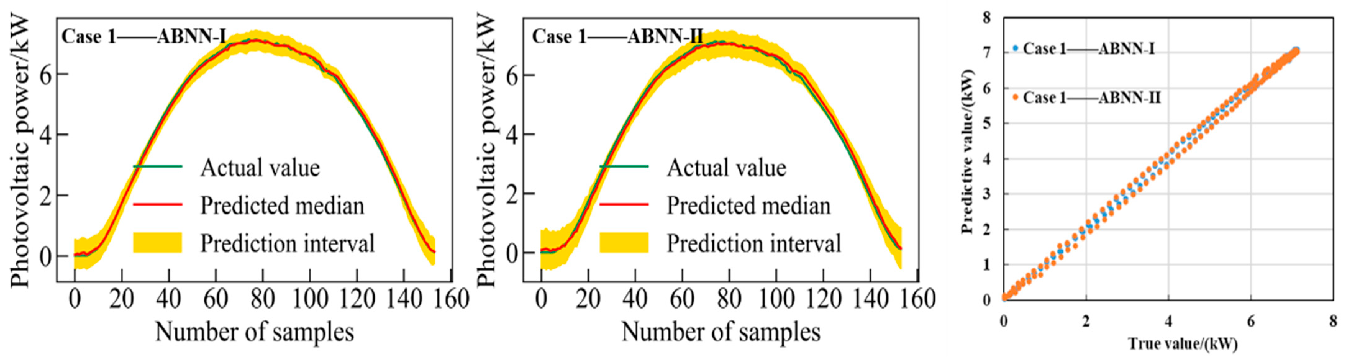
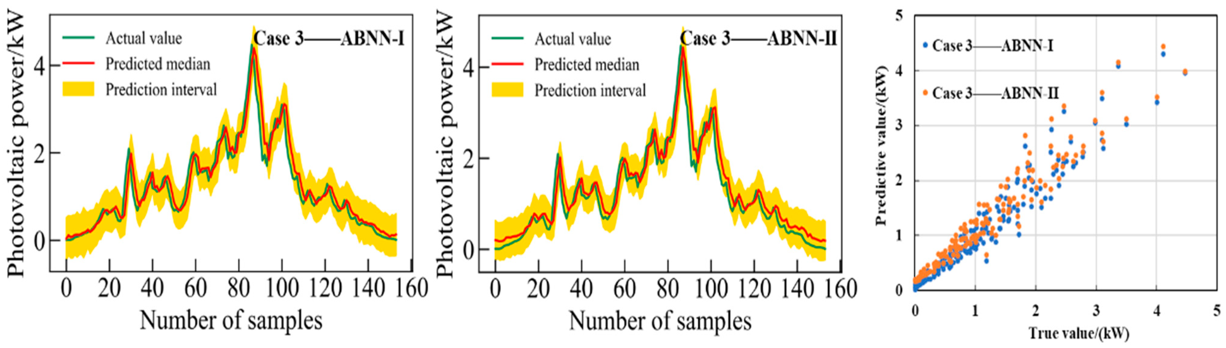
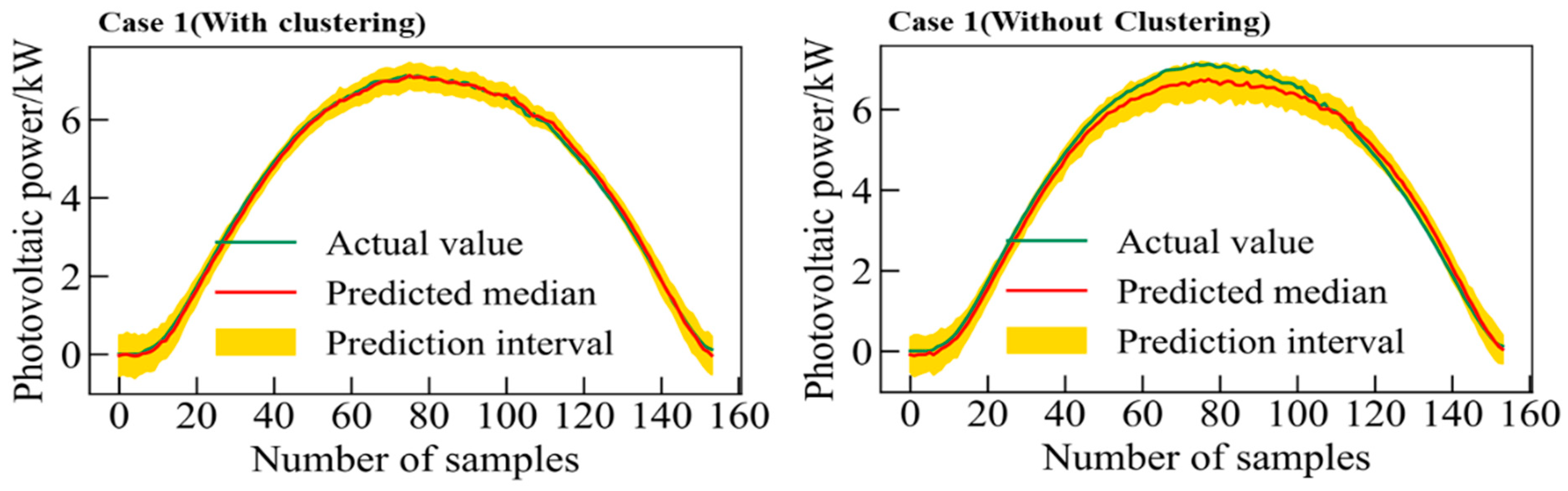
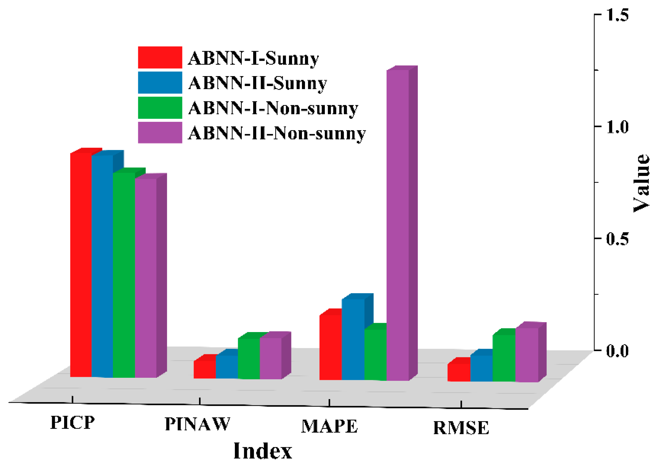