
Genetic Algorithms-Based Optimum PV Site Selection Minimizing Visual Disturbance


Abstract
1. Introduction
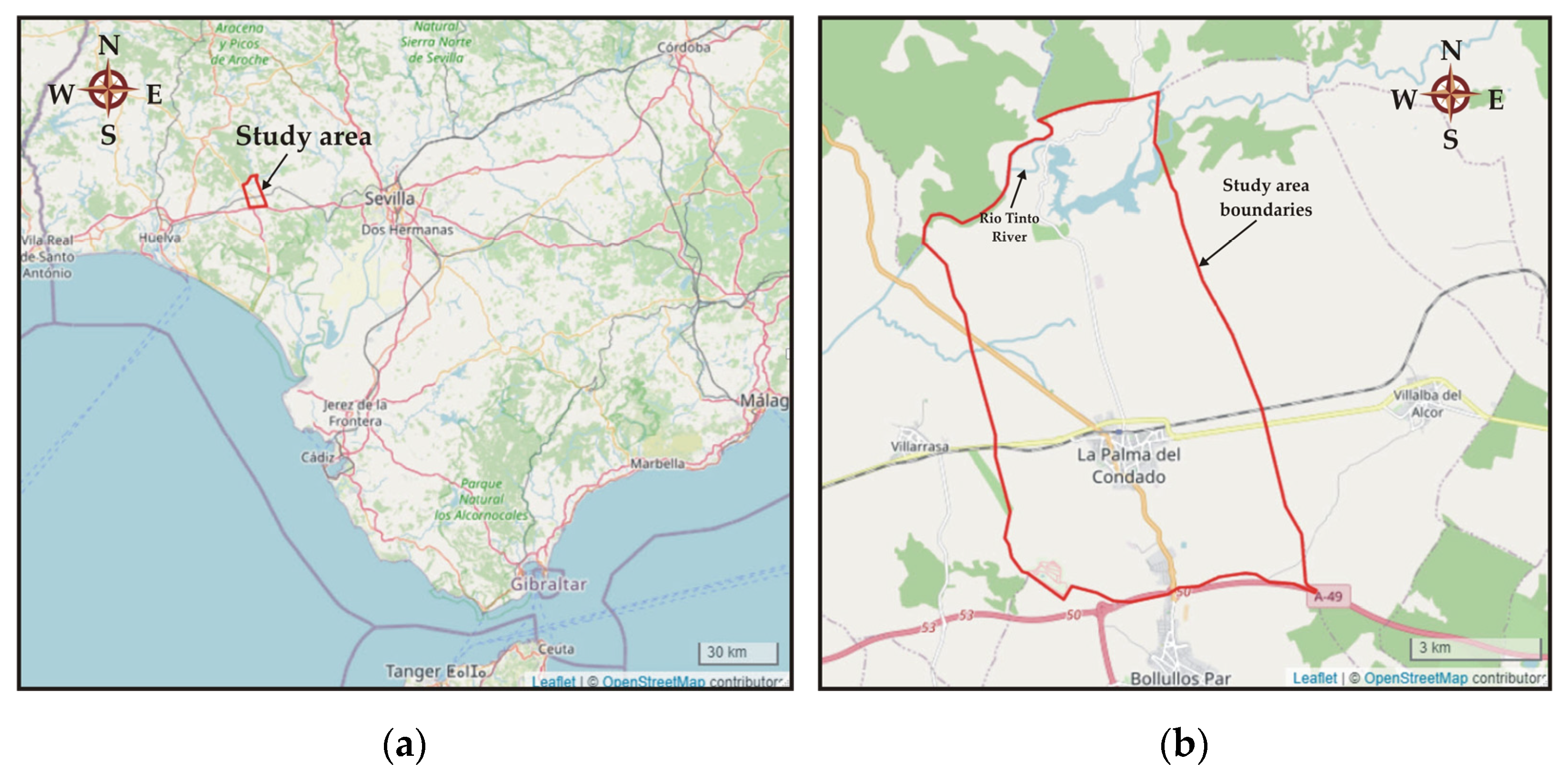
2. Study Area
3. Methodology
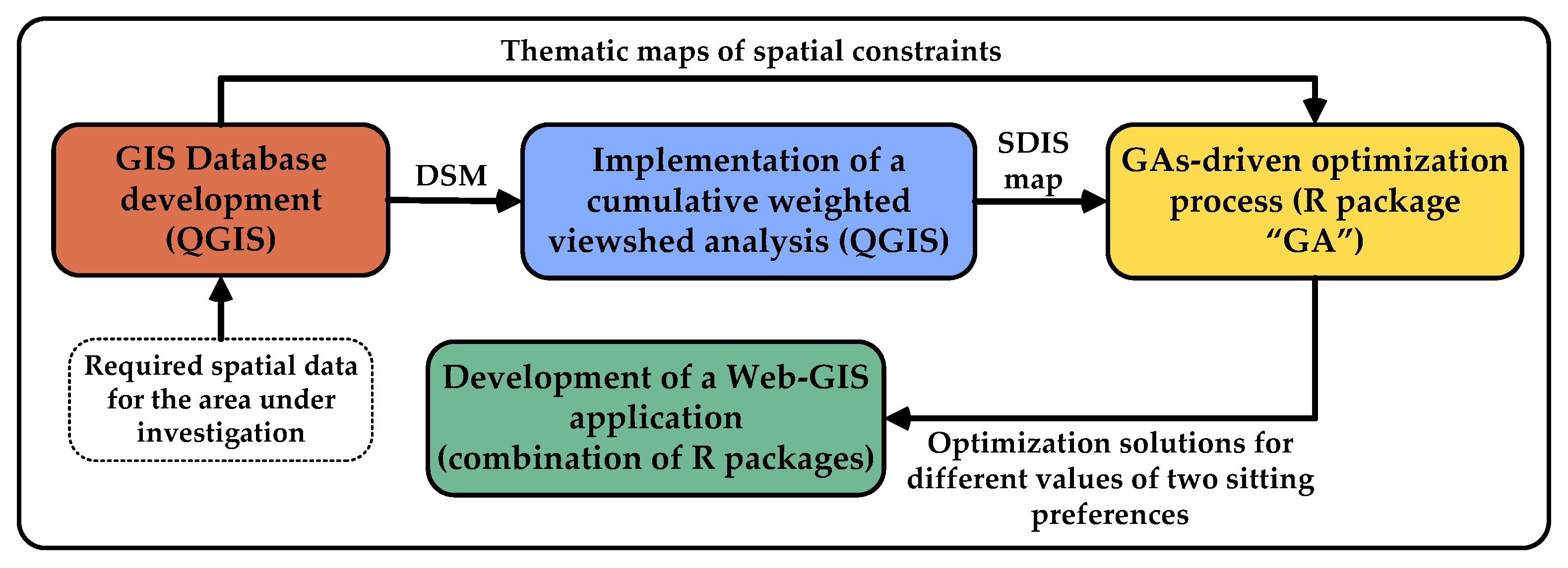
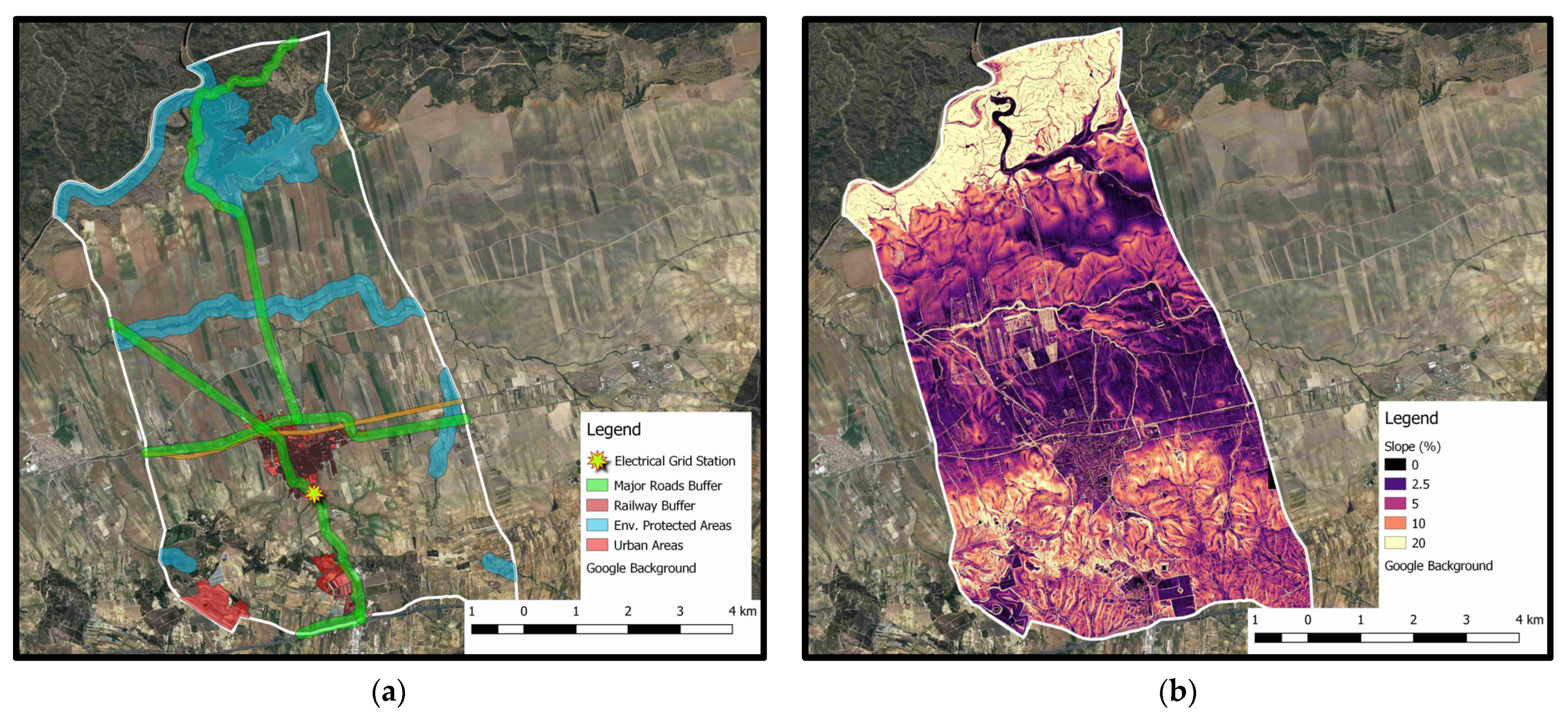
3.1. Development of the GIS Database
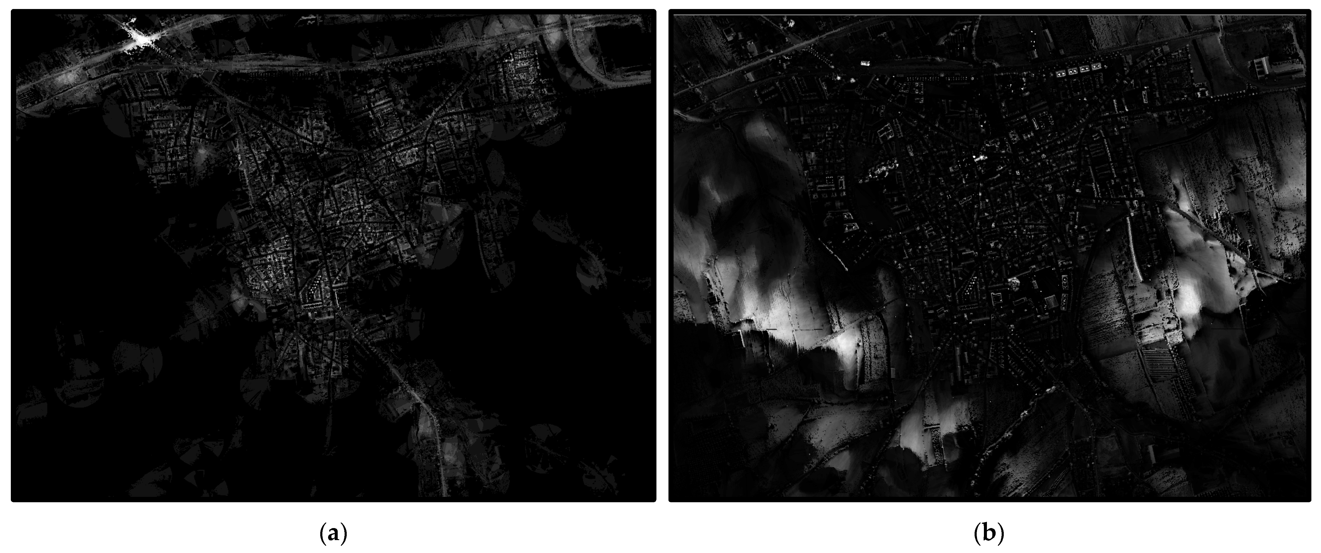
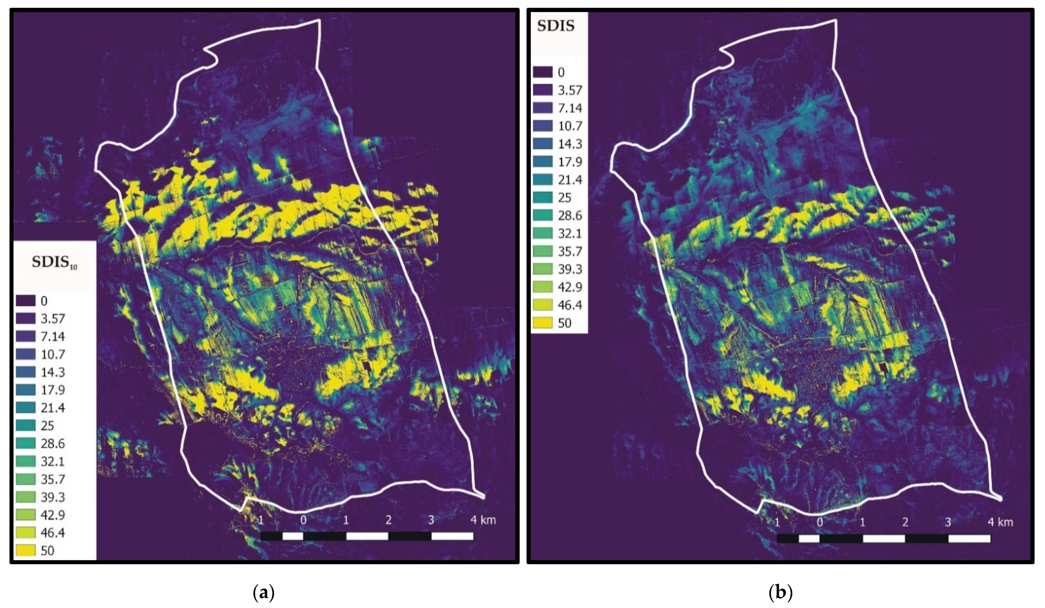
3.2. Vieswhed Analysis
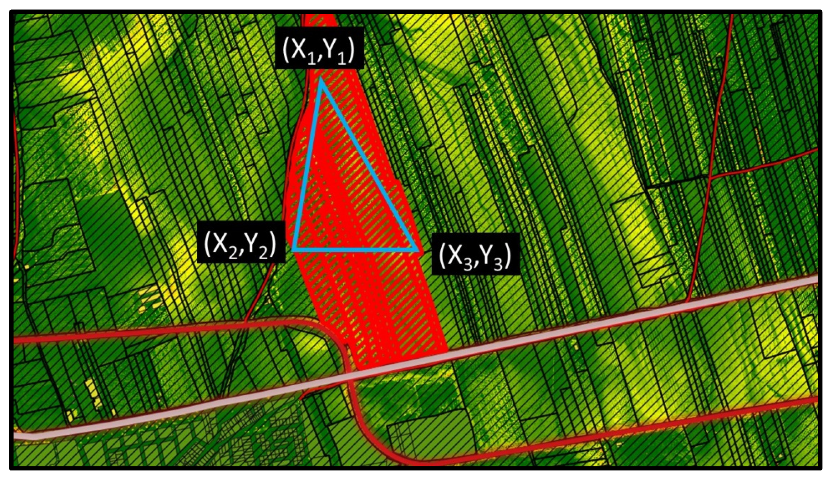
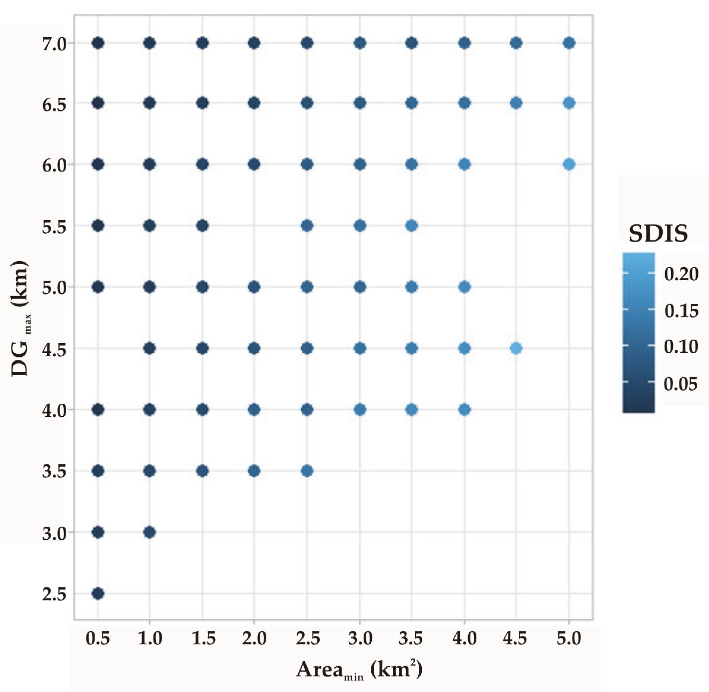
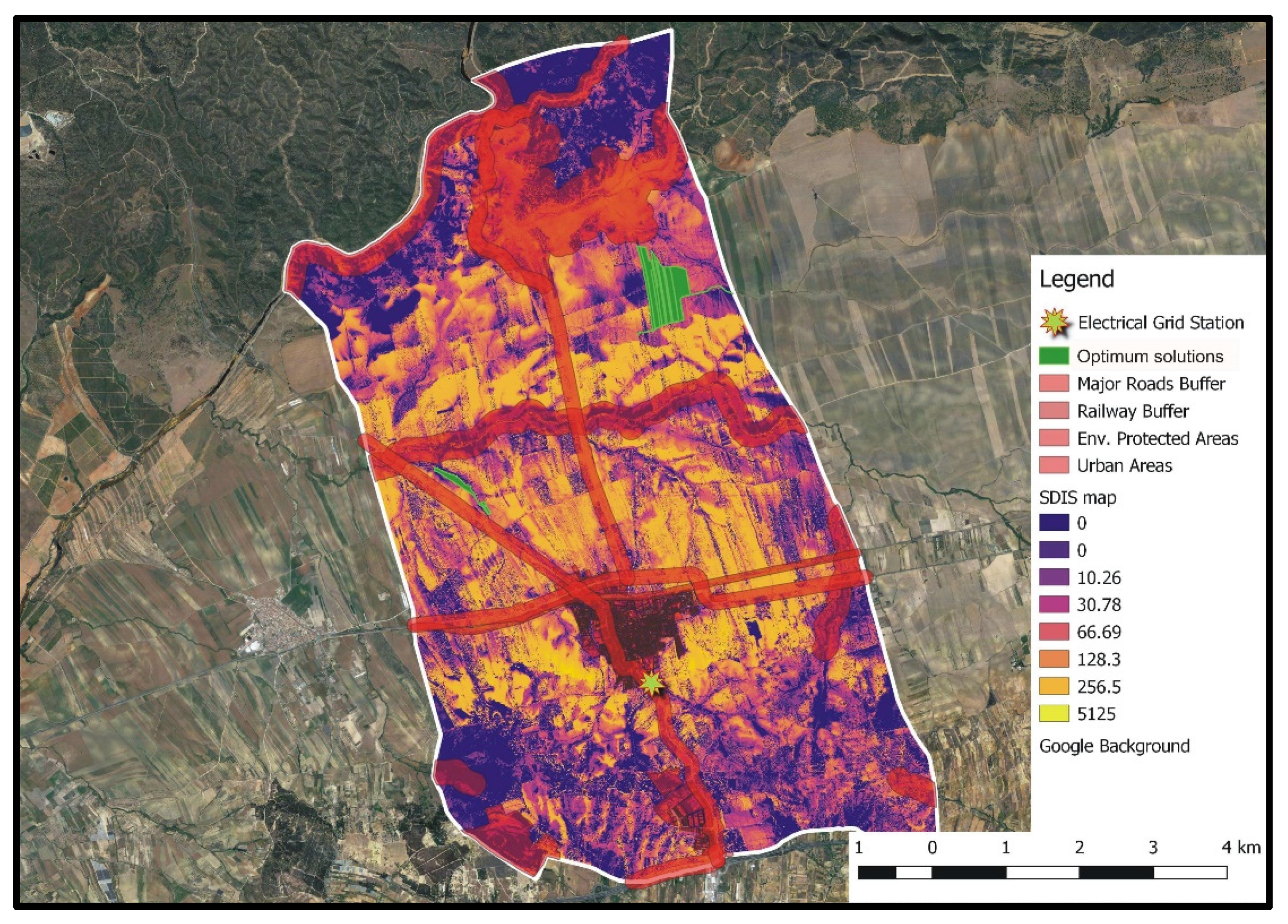
3.3. Optimization Process
4. Results and Discussion
5. Conclusions
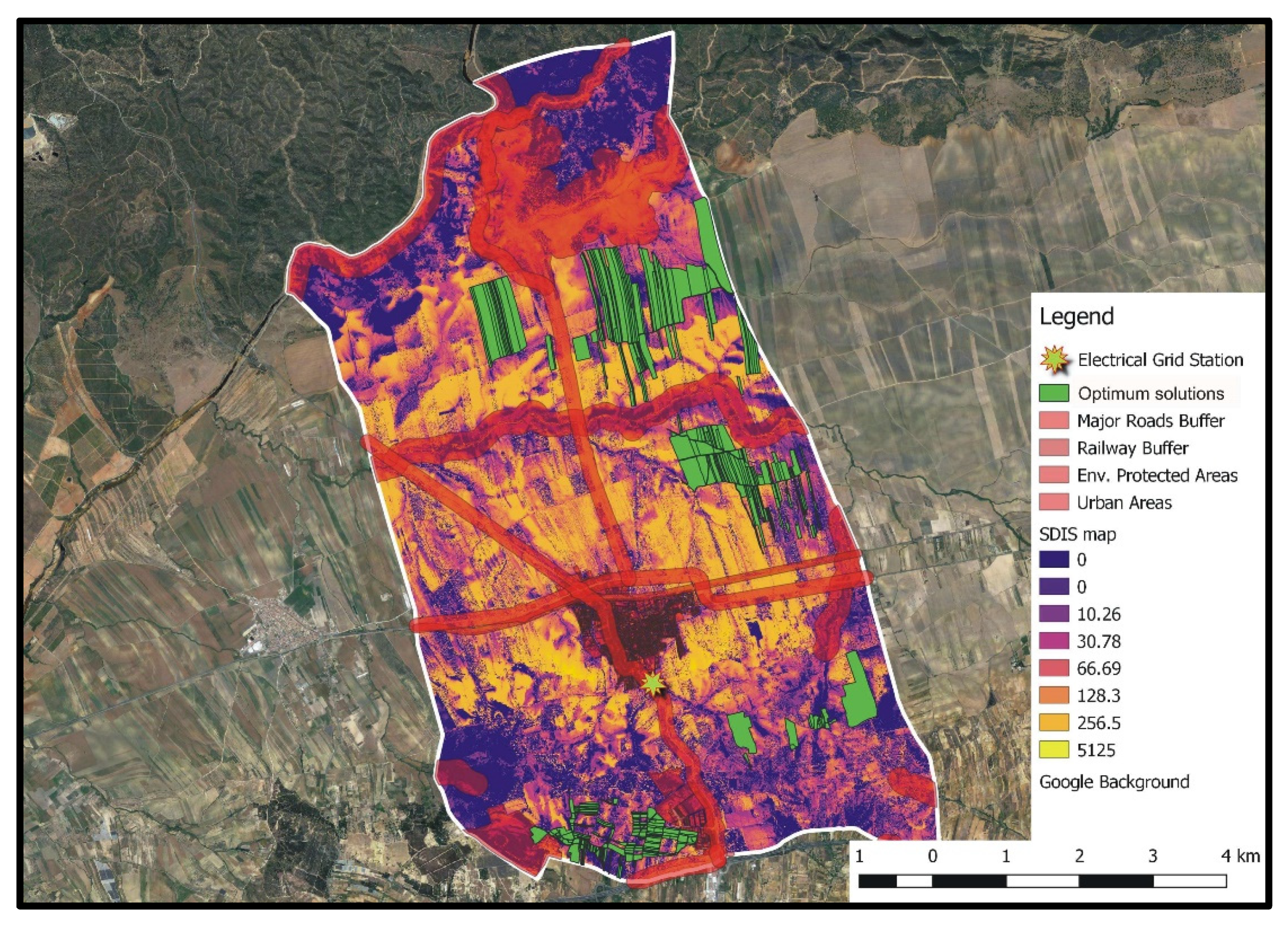
- The map of the proposed SDIS indicator can be easily created by both researchers and practitioners with low computational cost, and it accounts for the larger effect of the nearest objects on the visibility in an efficient manner. Accordingly, it can offer more realistic results than traditional viewsheds for assessing the visual effect of PV installations to the public.
- For a given DGmax value, the increase of Areamin facilitates the allocation of larger optimally suitable areas for installing PVs; thus, the aforementioned increase leads generally to larger SDIS values. The opposite holds true for DGmax, since, from a physical point of view, the increase of DGmax for a given Areamin value reduces the space suitable for PV installations.For the examined study area, the GAs-driven optimization process has led to empty optimum solution sets for numerous Areamin values, especially when DGmax ≤ 3.5 km, demonstrating that for small DGmax values, extensive areas for PV installations cannot be found in the region.
- The developed GAs-driven optimization process offers the ability to determine distinguishable, but compact, regions of optimum locations for PV installations within the examined region, facilitating relevant regional planning decisions. The consideration of the SDIS indicator in the objective function can contribute to the mitigation of potential social oppositions and negative impacts on land activities, since optimum areas correspond to those that will have the minimum visual impact to the community.
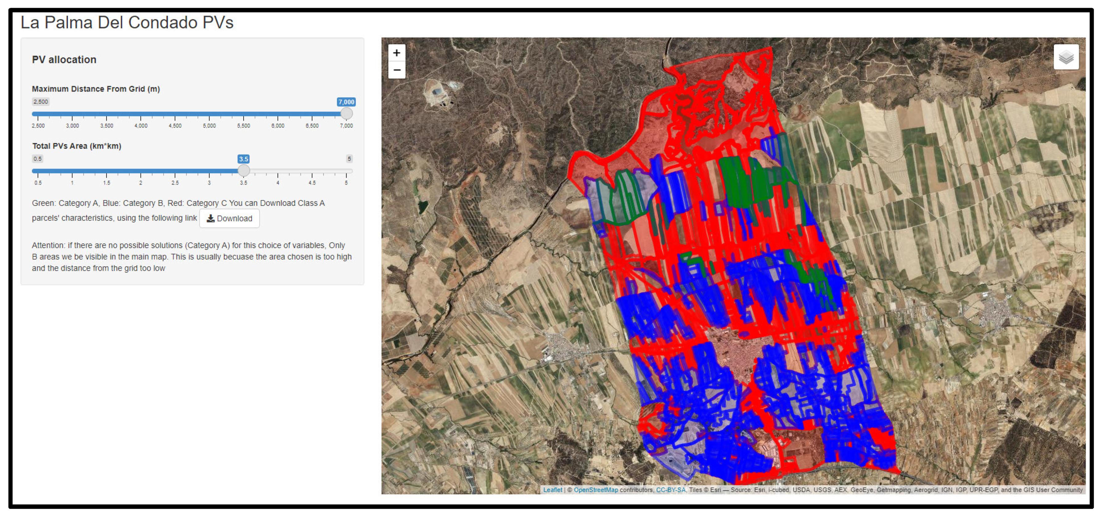
- The developed web-GIS application presents a flexible and easy-to-use tool that enables the visualization of PV plants’ optimum locations in the study area for different bounds of the PV locations—grid station in-between distance and of the PV locations’ total coverage area. Accordingly, it facilitates policy-makers to choose the set of solutions that better fulfils their preferences/strategies related to the above factors. The flexibility of the tool can also contribute to the reduction of bureaucracy, as well as to the further boost of the local solar energy market in an environmentally friendly and socially accepted manner.
Author Contributions
Funding
Institutional Review Board Statement
Informed Consent Statement
Data Availability Statement
Acknowledgments
Conflicts of Interest
Abbreviations
References
- Hussin, F.; Issabayeva, G.; Aroua, M.K. Solar photovoltaic applications: Opportunities and challenges. Rev. Chem. Eng. 2018, 34, 503–528. [Google Scholar] [CrossRef]
- Lefore, N.; Closas, A.; Schmitter, P. Solar for all: A framework to deliver inclusive and environmentally sustainable solar irrigation for smallholder agriculture. Energy Policy 2021, 154, 112313. [Google Scholar] [CrossRef]
- Delgado-Torres, A.M.; García-Rodríguez, L.; del Moral, M.J. Preliminary assessment of innovative seawater reverse osmosis (SWRO) desalination powered by a hybrid solar photovoltaic (PV)—Tidal range energy system. Desalination 2020, 477, 114247. [Google Scholar] [CrossRef]
- Hilarydoss, S. Suitability, sizing, economics, environmental impacts and limitations of solar photovoltaic water pumping system for groundwater irrigation—A brief review. Environ. Sci. Pollut. Res. 2021. [Google Scholar] [CrossRef] [PubMed]
- Toledo, C.; Scognamiglio, A. Agrivoltaic systems design and assessment: A critical review, and a descriptive model towards a sustainable landscape vision (three-dimensional agrivoltaic patterns). Sustainability 2021, 13, 6871. [Google Scholar] [CrossRef]
- Ren, Y.; Liu, X.; Li, H.; Qin, J.; Du, S.; Lu, X.; Tong, J.; Yang, C.; Li, J. Utilizing non-conjugated small-molecular tetrasodium iminodisuccinateas electron transport layer enabled improving efficiency of organic solar cells. Opt. Mater. 2022, 129, 112520. [Google Scholar] [CrossRef]
- Yang, C.; Zhang, C.; Chen, C.; Ren, Y.; Shen, H.; Tong, J.; Du, S.; Xia, Y.; Li, J. A new alcohol-soluble polymer PFN-ID as cathode interlayer to optimize performance of conventional polymer solar cells by increasing electron mobility. Energy Technol. 2022, 10, 2200199. [Google Scholar] [CrossRef]
- Yang, D. SolarData: An R package for easy access of publicly available solar datasets. Sol. Energy 2018, 171, A3–A12. [Google Scholar] [CrossRef]
- Ren, H.; Xu, C.; Ma, Z.; Sun, Y.A. novel 3D-geographic information system and deep learning integrated approach for high-accuracy building rooftop solar energy potential characterization of high-density cities. Appl. Energy 2022, 306, 117985. [Google Scholar] [CrossRef]
- Sun, T.; Shan, M.; Rong, X.; Yang, X. Estimating the spatial distribution of solar photovoltaic power generation potential on different types of rural rooftops using a deep learning network applied to satellite images. Appl. Energy 2022, 315, 119025. [Google Scholar] [CrossRef]
- Zhong, Q.; Nelson, J.R.; Tong, D.; Grubesic, T.H. A spatial optimization approach to increase the accuracy of rooftop solar energy assessments. Appl. Energy 2022, 316, 119128. [Google Scholar] [CrossRef]
- Raman, P.; Murali, J.; Sakthivadivel, D.; Vigneswaran, V.S. Opportunities and challenges in setting up solar photo voltaic based micro grids for electrification in rural areas of India. Renew. Sustain. Energy Rev. 2012, 16, 3320–3325. [Google Scholar] [CrossRef]
- Carvalho, P.C.; Machado, L.A.; Vitoriano, C.T.; Fernández Ramírez, L.M. Land Requirement Scenarios of PV Plants in Brazil. In Proceedings of the International Conference on Renewable Energies and Power Quality (ICREPQ’18), Salamanca, Spain, 21–23 March 2018. [Google Scholar]
- Mendas, A.; Delali, A. Integration of MultiCriteria Decision Analysis in GIS to develop land suitability for agriculture: Application to durum wheat cultivation in the region of Mleta in Algeria. Comput. Electron. Agric. 2012, 83, 117–126. [Google Scholar] [CrossRef]
- Guaita-Pradas, I.; Marques-Perez, I.; Gallego, A.; Segura, B. Analyzing territory for the sustainable development of solar photovoltaic power using GIS databases. Environ. Monit. Assess. 2019, 191, 764. [Google Scholar] [CrossRef]
- Lindberg, O.; Birging, A.; Widén, J.; Lingfors, D. PV park site selection for utility-scale solar guides combining GIS and power flow analysis: A case study on a Swedish municipality. Appl. Energy 2021, 282, 116086. [Google Scholar] [CrossRef]
- Zoellner, J.; Schweizer-Ries, P.; Wemheuer, C. Public acceptance of renewable energies: Results from case studies in Germany. Energy Policy 2008, 36, 4136–4141. [Google Scholar] [CrossRef]
- Brewer, J.; Ames, D.P.; Solan, D.; Lee, R.; Carlisle, J. Using GIS analytics and social preference data to evaluate utility-scale solar power site suitability. Renew. Energy 2015, 81, 825–836. [Google Scholar] [CrossRef]
- Scognamiglio, S. ‘Photovoltaic landscapes’: Design and assessment. A critical review for a new transdisciplinary design vision. Renew. Sustain. Energy Rev. 2016, 55, 629–661. [Google Scholar] [CrossRef]
- Díez-Mediavilla, M.; Alonso-Tristán, C.; Rodríguez-Amigo, M.C.; García-Calderón, T. Implementation of PV plants in Spain: A case study. Renew. Sustain. Energy Rev. 2010, 14, 1342–1346. [Google Scholar] [CrossRef]
- Coronas, S.; de la Hoz, J.; Alonso, À.; Martín, H. 23 years of development of the solar power generation sector in Spain: A comprehensive review of the period 1998–2020 from a regulatory perspective. Energies 2022, 15, 1593. [Google Scholar] [CrossRef]
- Gabaldón-Estevan, D.; Peñalvo-López, E.; Alfonso Solar, D. The Spanish turn against renewable energy development. Sustainability 2018, 10, 1208. [Google Scholar] [CrossRef]
- Ibarloza, A.; Heras-Saizarbitoria, I.; Allur, E.; Larrea, A. Regulatory cuts and economic and financial performance of Spanish solar power companies: An empirical review. Renew. Sustain. Energy Rev. 2018, 92, 784–793. [Google Scholar] [CrossRef]
- de la Hoz, J.; Martín, H.; Martins, B.; Matas, J.; Miret, J. Evaluating the impact of the administrative procedure and the landscape policy on grid connected PV systems (GCPVS) on-floor in Spain in the period 2004–2008: To which extent a limiting factor? Energy Policy 2013, 63, 147–167. [Google Scholar] [CrossRef]
- Fisher, P.F. First experiments in viewshed uncertainty: Simulating fuzzy viewsheds. Photogramm. Eng. Remote Sens. 1992, 58, 345. [Google Scholar]
- Nutsford, D.; Reitsma, F.; Pearson, A.L.; Kingham, S. Personalising the viewshed: Visibility analysis from the human perspective. Appl. Geogr. 2015, 62, 1–7. [Google Scholar] [CrossRef]
- Wheatley, D. Cumulative viewshed analysis: A GIS-based method for investigating intervisibility, and its archaeological application. In Archaeology and Geographic Information Systems: A European Perspective; Lock, G., Stancic, Z., Eds.; Taylor and Francis: London, UK, 1995; pp. 171–186. [Google Scholar]
- Loots, L.; Nackaerts, K.; Waelkens, M. Fuzzy Viewshed Analysis of the Hellenistic City Defence System at Sagalassos, Turkey. In Proceedings of the 25th Anniversary Conference of Computer Applications and Quantitative Methods in Archaeology (CAA 1997), Birmingham, UK, 10–17 April 1997. [Google Scholar]
- Hognogi, G.G.; Pop, A.M.; Mălăescu, S.; Nistor, M.M. Increasing territorial planning activities through viewshed analysis. Geocarto Int. 2022, 37, 627–637. [Google Scholar] [CrossRef]
- Inglis, N.C.; Vukomanovic, J.; Costanza, J.; Singh, K.K. From viewsheds to viewscapes: Trends in landscape visibility and visual quality research. Landsc. Urban Plan. 2022, 224, 104424. [Google Scholar] [CrossRef]
- Labib, S.M.; Huck, J.J.; Lindley, S. Modelling and mapping eye-level greenness visibility exposure using multi-source data at high spatial resolutions. Sci. Total Environ. 2021, 755, 143050. [Google Scholar] [CrossRef]
- Zorzano-Alba, E.; Fernandez-Jimenez, L.A.; Garcia-Garrido, E.; Lara-Santillan, P.M.; Falces, A.; Zorzano-Santamaria, P.J.; Capellan-Villacian, C.; Mendoza-Villena, M. Visibility assessment of new photovoltaic power plants in areas with special landscape value. Appl. Sci. 2022, 12, 703. [Google Scholar] [CrossRef]
- Fisher, P.F. Algorithm and implementation uncertainty in viewshed analysis. Int. J. Geogr. Inf. Syst. 1993, 7, 331–347. [Google Scholar] [CrossRef]
- Klouček, T.; Lagner, O.; Šímová, P. How does data accuracy influence the reliability of digital viewshed models? A case study with wind turbines. Appl. Geogr. 2015, 64, 46–54. [Google Scholar] [CrossRef]
- Garré, S.; Meeus, S.; Gulinck, H. The dual role of roads in the visual landscape: A case-study in the area around Mechelen (Belgium). Landsc. Urban Plan. 2009, 92, 125–135. [Google Scholar] [CrossRef]
- Parsons, B.M.; Coops, N.C.; Stenhouse, G.B.; Burton, A.C.; Nelson, T.A. Building a perceptual zone of influence for wildlife: Delineating the effects of roads on grizzly bear movement. Eur. J. Wildl. Res. 2020, 66, 53. [Google Scholar] [CrossRef]
- Fernandez-Jimenez, L.A.; Mendoza-Villena, M.; Zorzano-Santamaria, P.; Garcia-Garrido, E.; Lara-Santillan, P.; Zorzano-Alba, E.; Falces, A. Site selection for new PV power plants based on their observability. Renew. Energy 2015, 78, 7–15. [Google Scholar] [CrossRef]
- Holland, J.H. Adaptation in Natural and Artificial Systems; MIT Press: Cambridge, MA, USA, 1975. [Google Scholar]
- Deb, K. Multi-Objective Optimization Using Evolutionary Algorithms; John Wiley & Sons: New York, NY, USA, 2001. [Google Scholar]
- Katsifarakis, K.L.; Kontos, Y.N. Genetic algorithms: A mature mio-inspired optimization technique for difficult problems. In Nature-Inspired Methods for Metaheuristics Optimization: Algorithms and Applications in Science and Engineering, Modeling and Optimization in Science and Technologies; Bennis, F., Bhattacharjya, R.K., Eds.; Springer International Publishing: Cham, Switzerland, 2020; Volume 16, pp. 3–25. [Google Scholar] [CrossRef]
- Albadi, M.H.; Al-Hinai, A.S.; Al-Abri, N.N.; Al-Busafi, Y.H.; Al-Sadairi, R.S. Optimal allocation of solar PV systems in rural areas using genetic algorithms: A case study. Int. J. Sustain. Eng. 2013, 6, 301–306. [Google Scholar] [CrossRef]
- Vermeulen, V.; Strauss, J.M.; Vermeulen, H.J. Optimisation of Solar PV Plant Locations for Grid Support using Genetic Algorithm and Pattern Search. In Proceedings of the 2016 IEEE International Conference on Power and Energy (PECon 2016), Melaka City, Malaysia, 28–30 November 2016. [Google Scholar]
- Masoum, M.A.; Badejani, S.M.M.; Kalantar, M. Optimal Placement of Hybrid PV-wind Systems using Genetic Algorithm. In Proceedings of the 2010 Innovative Smart Grid Technologies (ISGT), Gaithersburg, MD, USA, 19–21 January 2010. [Google Scholar]
- Yanık, S.; Sürer, Ö.; Öztayşi, B. Designing sustainable energy regions using genetic algorithms and location-allocation approach. Energy 2016, 97, 161–172. [Google Scholar] [CrossRef]
- Institute of Statistics and Cartography of Andalucia. Available online: https://www.juntadeandalucia.es/institutodeestadisticaycartografia/sima/ficha.htm?mun=21054 (accessed on 4 September 2022).
- Carrión, J.A.; Espín Estrella, A.; Aznar Dols, F.; Ridao, A.R. The electricity production capacity of photovoltaic power plants and the selection of solar energy sites in Andalusia (Spain). Renew. Energy 2008, 33, 545–552. [Google Scholar] [CrossRef]
- European Commission, Natura2000. Available online: https://www.eea.europa.eu/data-and-maps/data/natura-13/natura-2000-spatial-data (accessed on 4 September 2022).
- Spanish National Georaphic Institute. Available online: http://centrodedescargas.cnig.es/CentroDescargas/locale?request_locale=es (accessed on 4 September 2022).
- Spyridonidou, S.; Sismani, G.; Loukogeorgaki, E.; Vagiona, D.G.; Ulanovsky, H.; Madar, D. Sustainable spatial energy planning of large-scale wind and PV farms in Israel: A collaborative and participatory planning approach. Energies 2021, 14, 551. [Google Scholar] [CrossRef]
- Uyan, M. GIS-based solar farms site selection using analytic hierarchy process (AHP) in Karapinar region, Konya/Turkey. Renew. Sustain. Energy Rev. 2013, 28, 11–17. [Google Scholar] [CrossRef]
- Gašparović, I.; Gašparović, M. Determining optimal solar power plant locations based on remote sensing and GIS methods: A case study from Croatia. Remote Sens. 2019, 11, 1481. [Google Scholar] [CrossRef]
- Arán Carrión, J.; Espín Estrella, A.; Aznar Dols, F.; Zamorano Toro, M.; Rodríguez, M.; Ramos Ridao, A. Environmental decision-support systems for evaluating the carrying capacity of land areas: Optimal site selection for grid-connected photovoltaic power plants. Renew. Sustain. Energy Rev. 2008, 12, 2358–2380. [Google Scholar] [CrossRef]
- Tercan, E.; Saracoglu, B.O.; Bilgilioğlu, S.S.; Eymen, A.; Tapkın, S. Geographic information system-based investment system for photovoltaic power plants location analysis in Turkey. Environ. Monit. Assess. 2020, 192, 297. [Google Scholar] [CrossRef]
- Tahri, M.; Hakdaoui, M.; Maanan, M. The evaluation of solar farm locations applying Geographic Information System and Multi-Criteria Decision-Making methods: Case study in southern Morocco. Renew. Sustain. Energy Rev. 2015, 51, 1354–1362. [Google Scholar] [CrossRef]
- Roussel, J.R.; Auty, D.; Coops, N.C.; Tompalski, P.; Goodbody, T.R.H.; Meador, A.S.; Bourdon, J.F.; de Boissieu, F.; Achim, A. lidR: An R package for analysis of Airborne Laser Scanning (ALS) data. Remote Sens. Environ. 2020, 251, 112061. [Google Scholar] [CrossRef]
- Šúri, M.; Huld, T.A.; Dunlop, E.D. PV-GIS: A web-based solar radiation database for the calculation of PV potential in Europe. Int. J. Sustain. Energy 2005, 24, 55–67. [Google Scholar] [CrossRef]
- Cuckovic, Z. Advanced viewshed analysis: A Quantum GIS plug-in for the analysis of visual landscapes. J. Open Source Softw. 2016, 1, 32. [Google Scholar] [CrossRef]
- Fishburn, P.C. Utility Theory for Decision Making; Research Analysis Corporation: McLean Virginia, VA, USA, 1970. [Google Scholar]
- Kumsap, C.; Borne, F.; Moss, D. The technique of distance decayed visibility for forest landscape visualization. Int. J. Geogr. Inf. Sci. 2005, 19, 723–744. [Google Scholar] [CrossRef]
- Chen, Z.; Xu, B.; Gao, B. Assessing visual green effects of individual urban trees using airborne Lidar data. Sci. Total Environ. 2015, 536, 232–244. [Google Scholar] [CrossRef] [PubMed]
- Bunke, H. Graph Matching: Theoretical Foundations, Algorithms, and Applications. In Proceedings of the Vision Interface Conference (VI’2000), Montréal, QC, Canada, 14–17 May 2000. [Google Scholar]
- Scrucca, L. On some extensions to GA package: Hybrid optimisation, parallelisation and islands evolution. R J. 2017, 9, 187–206. [Google Scholar] [CrossRef]
- Shiny: Web Application Framework for R. Available online: https://CRAN.R-project.org/package=shiny (accessed on 4 September 2022).
- LeafletR: Open-Source JavaScript Library for Mobile-Friendly Interactive Maps, R Package Version 0.4-0. Available online: https://cran.r-project.org/src/contrib/Archive/leafletR/ (accessed on 4 September 2022).
- Tennekes, M. tmap: Thematic Maps in R. J. Stat. Softw. 2018, 84, 1–39. [Google Scholar] [CrossRef]
- Plotly: R Package for Creating Interactive Web-Based Graphs via the Open Source JavaScript Graphing Library. Available online: https://plot.ly (accessed on 4 September 2022).


| ID | Criterion | Incompatibility Zones | Spatial Data Source |
|---|---|---|---|
| EC1 | Distance from environmentally protected areas (Natura 2000 areas) | ≤150 m | [47] |
| EC2 | Distance from major roads | ≤100 m | La Palma Del Condado municipality (personal communication) |
| EC3 | Distance from railway network | ≤50 m | |
| EC4 | Land use | Non-agricultural areas and vineyards | |
| EC5 | Slope of terrain | ≥5% | [48] |
| j | 1 | 2 | 3 | 4 | 5 | 6 | 7 | 8 | 9 | 10 |
|---|---|---|---|---|---|---|---|---|---|---|
| rj (m) | 100 | 200 | 300 | 400 | 500 | 1000 | 1500 | 2000 | 3500 | 5000 |
| cj | 4.912 | 4.219 | 3.813 | 3.526 | 3.303 | 2.609 | 2.204 | 1.916 | 1.357 | 1.000 |
| No. | Feature | Set A | Set B | Set C | |
|---|---|---|---|---|---|
| 1 | EC1 satisfaction | No | No | No | Yes |
| 2 | EC2 satisfaction | ||||
| 3 | EC3 satisfaction | ||||
| 4 | EC4 satisfaction | Yes (vineyards) | Partial (only non-agricultural areas are included) | ||
| 5 | EC5 satisfaction | Yes | Not examined | ||
| 6 | Minimum SDIS indicator | Yes | No | Not examined | Not examined |
| 7 | Distance from grid station smaller than a predefined upper bound | ||||
| 8 | PV locations’ total coverage area larger than a predefined low bound | ||||
| Areamin Values (km2) | DGmax Values (km) | |||||||||
|---|---|---|---|---|---|---|---|---|---|---|
| 2.5 | 3.0 | 3.5 | 4.0 | 4.5 | 5.0 | 5.5 | 6.0 | 6.5 | 7.0 | |
| 0.5 | 0.022 | 0.025 | 0.024 | 0.009 | 25.000 | 0.011 | 0.010 | 0.009 | 0.006 | 0.006 |
| 1.0 | 5.000 | 0.048 | 0.044 | 0.033 | 0.028 | 0.020 | 0.029 | 0.019 | 0.018 | 0.017 |
| 1.5 | 7.500 | 7.500 | 0.070 | 0.051 | 0.042 | 0.045 | 0.037 | 0.039 | 0.028 | 0.025 |
| 2.0 | 10.000 | 10.000 | 0.101 | 0.091 | 0.067 | 0.065 | 60.000 | 0.052 | 0.038 | 0.034 |
| 2.5 | 12.500 | 12.500 | 0.128 | 0.094 | 0.089 | 0.097 | 0.100 | 0.081 | 0.064 | 0.048 |
| 3.0 | 15.000 | 15.000 | 15.000 | 0.140 | 0.120 | 0.104 | 0.122 | 0.096 | 0.082 | 0.077 |
| 3.5 | 17.500 | 17.500 | 17.500 | 0.163 | 0.147 | 0.139 | 0.159 | 0.125 | 0.101 | 0.071 |
| 4.0 | 20.000 | 20.000 | 20.000 | 0.168 | 0.170 | 0.165 | 20.000 | 0.157 | 0.118 | 0.093 |
| 4.5 | 45.000 | 22.500 | 22.500 | 22.500 | 0.229 | 22.500 | 22.500 | 22.500 | 0.148 | 0.109 |
| 5.0 | 50.000 | 150.000 | 25.000 | 25.000 | 25.000 | 25.000 | 25.000 | 0.204 | 0.178 | 0.124 |
Publisher’s Note: MDPI stays neutral with regard to jurisdictional claims in published maps and institutional affiliations. |
© 2022 by the authors. Licensee MDPI, Basel, Switzerland. This article is an open access article distributed under the terms and conditions of the Creative Commons Attribution (CC BY) license (https://creativecommons.org/licenses/by/4.0/).
Share and Cite
Nagkoulis, N.; Loukogeorgaki, E.; Ghislanzoni, M. Genetic Algorithms-Based Optimum PV Site Selection Minimizing Visual Disturbance. Sustainability 2022, 14, 12602. https://doi.org/10.3390/su141912602
Nagkoulis N, Loukogeorgaki E, Ghislanzoni M. Genetic Algorithms-Based Optimum PV Site Selection Minimizing Visual Disturbance. Sustainability. 2022; 14(19):12602. https://doi.org/10.3390/su141912602
Chicago/Turabian StyleNagkoulis, Nikolaos, Eva Loukogeorgaki, and Michela Ghislanzoni. 2022. "Genetic Algorithms-Based Optimum PV Site Selection Minimizing Visual Disturbance" Sustainability 14, no. 19: 12602. https://doi.org/10.3390/su141912602
APA StyleNagkoulis, N., Loukogeorgaki, E., & Ghislanzoni, M. (2022). Genetic Algorithms-Based Optimum PV Site Selection Minimizing Visual Disturbance. Sustainability, 14(19), 12602. https://doi.org/10.3390/su141912602