Spatiotemporal Response of Ecosystem Service Values to Land Use Change in Xiamen, China

Abstract

This research aims to identify the key indicators of land-use change that affect ecosystem service in the coastal city of Xiamen. The methods of transfer matrix and land-use dynamic degree are used to analyze land-use change, and the spatial distribution of ecosystem service values (ESV) is mapped from 1989 to 2018 using cluster analysis. During this 30-year period, the built-up land expanded rapidly through occupation of farmland and landfilling of the watershed. The biggest contribution to the reduction of ESV in this stage is the loss of farmland followed by the loss of watershed. By 2018, the spatial distribution of ESV had become very unbalanced and polarized. The high-value areas are mainly distributed in the northern mountainous areas, with the low-value areas concentrated in the flat areas near the coastline, and only a few medium-value areas of ESV remained. Generally, from 1989 to 2018, the ESV in Xiamen decreased by about CNY 200 million in total, with the largest proportion of ESV reduction (CNY 120 million) occurring in the 2000–2010 period. Considering ESV categories, the significant reduction of Regulating Service (53.5–57.8%) was mainly due to the loss of water areas (CNY −70 million) to low ESV areas (built-up land) in urbanization, followed by the loss of farmland (CNY −50 million). This means that Xiamen should strengthen the protection of ecological lands in future urban planning to alleviate and reverse the current ecological imbalance.

1. Introduction

Land-use and land-cover change (LULCC) is a key component of global environmental change because it drives changes in ecosystem service function, affecting the type, area and spatial distribution pattern of ecosystems [1,2]. Ecosystem services (ESs) are also essential measures of regional sustainable development [3,4,5]. Land-use change greatly affects the ecosystem function by changing environmental biophysical factors such as biodiversity, thus influencing ESs [3,6,7]. In turn, the degradation or loss of ecosystem services affects the structure and efficiency of land use and human sustainable development [8,9].

In order to achieve an improved balance in land-use planning and regional sustainable development into the future, the impacts of rapid urbanization and land-use change on ESV need to be studied in more detail [10]. Moreover, in order to protect and increase the total regional ESV, as well as optimization of the ESV spatial pattern through land planning in the future, the study of the spatial pattern of ESV and its response to land-use change is necessary [11,12].

Since Costanza proposed the principle and method of ESV estimation and calculated the economic value of global ESV in 1997 [3], many international scholars have continuously explored and improved the theoretical research of ESV [13,14]. Among them, Polasky et al. conducted empirical research about the impact of land-use change on ESV [15,16].

Costanza provided the principles, methods and all aspects about the ESV estimation, estimated and calculated the global ESV. However, his estimation and calculation would not be entirely applicable to China considering the scale effect and differences. Regions with different conditions have different ecological benefit in the same type of land use, and the ESV is highly related to local living standards [17]. Since the equivalent value per unit area varies widely, using the global equivalent value set up by Costanza for China would make the results much higher than what these may be in reality [17]. Thus, the equivalent coefficient needs to be adjusted when conducting analysis in special regions considering the actual situation to obtain more accurate result.

Since the 1978 reform and opening policy, China has experienced rapid industrialization and accelerated urbanization development with explosive population growth over four decades, resulting in significant changes in LULCC [18,19], especially farmland transition to built-up land [20,21]. With urban economic development stimulus, rural–urban migration promoted the built-up land increasing. However, for a long time, such urban land expansion by encroachment on farmland was at a rate even faster than the increase in urban population [22]. Meanwhile, widespread transition of farmland to urban area correspondingly reduced the physical supply of ecosystem services [23], had significant negative impacts on ecosystem services [24,25] and reduced the value of ecosystem services [26,27,28].

Research on ESV in China mainly focused on two aspects. On one hand, some scholars focused on ESV evaluation methods [29,30,31]. The evaluation system established by Xie in 2006 and its improved methods have been accepted and used by many scholars [17,25,32,33]. On the other hand, others have applied the ESV evaluation method in various fields or linked it with other concepts to conduct theoretical or case studies [34,35,36].

Considering current research, few of these focus on the spatial pattern and temporal evolution of ESV and the sensitivity or response of ESV to land-use change. Future land planning guided by such research could help optimize the urban land spatial pattern and sustainable development. For ESV spatial pattern and its response to the land use, Sannigrahi conducted a global scale study using the coefficient of sensitivity and elasticity [37]. Akhtar investigated the historical LUCC with ESV, and then simulated the future of them. However, this research did not consider the spatial distribution of ESV change due to land-use transition and the spatial pattern of the ESV sub-category [11].

Some scholars conducted research on the spatial pattern of ESV change due to land-use change in Northwest China, and some of them simulated the ESV change based on future land-planning scenarios [12,38,39]. However, these studies are not comprehensive. For instance, the research in Ningxia did not analyze the ESV spatial pattern in time nodes and periods [12]; although research in Gansu and Xinjiang included analyses in time periods and nodes, respectively, neither of these analyzed the spatial distribution of ESV sub-categories [38,39]. Similarly, research in Fujian province and Hangzhou Bay in the southern and eastern parts of China did not analyze the spatial pattern of ESV [40,41]. Finally, research in Guangdong and Guangxi provinces did not include an analysis of the spatial distribution of ESV loss or gain due to land-use change [42,43].

In the present research, the coastal city of Xiamen, also known by its English name ‘Amoy’, was selected as the study area to analyze the land-use evolution and its impact on ESV. After being set up as one of the five Special Economic Zones in the 1980s, Xiamen experienced rapid economic development through industrialization and urbanization [44]. This has been viewed to have had a pioneering and influential role in the surrounding regions and even in the whole country. In the Seventh National Census in 2020, the urbanization rate of Xiamen had reached an astonishing 89.4%, even higher than the top developed city of Shanghai (urbanization rate of 89.3%). The rapid urban development has exerted great pressure on the eco-environment health of Xiamen [45]. At present, China advocates the concept of Ecological Civilization development. How to balance industrialization, urbanization and urban eco-environment health in Xiamen is an important issue for sustainable development. While the previous studies on land-use change and ESV in Xiamen mainly focused on structural analysis, research on the spatial pattern and the impacts of land-use change on ESV is yet to be carried out.

Thus, this paper focuses on how the spatial distribution and related characteristics of ESV was affected by land-use transition and patterns over a 30 year period, especially in the case of one of the first cities in the world that has gone through a very rapid urbanization process in a relatively short period of time.

2. Materials and Methods

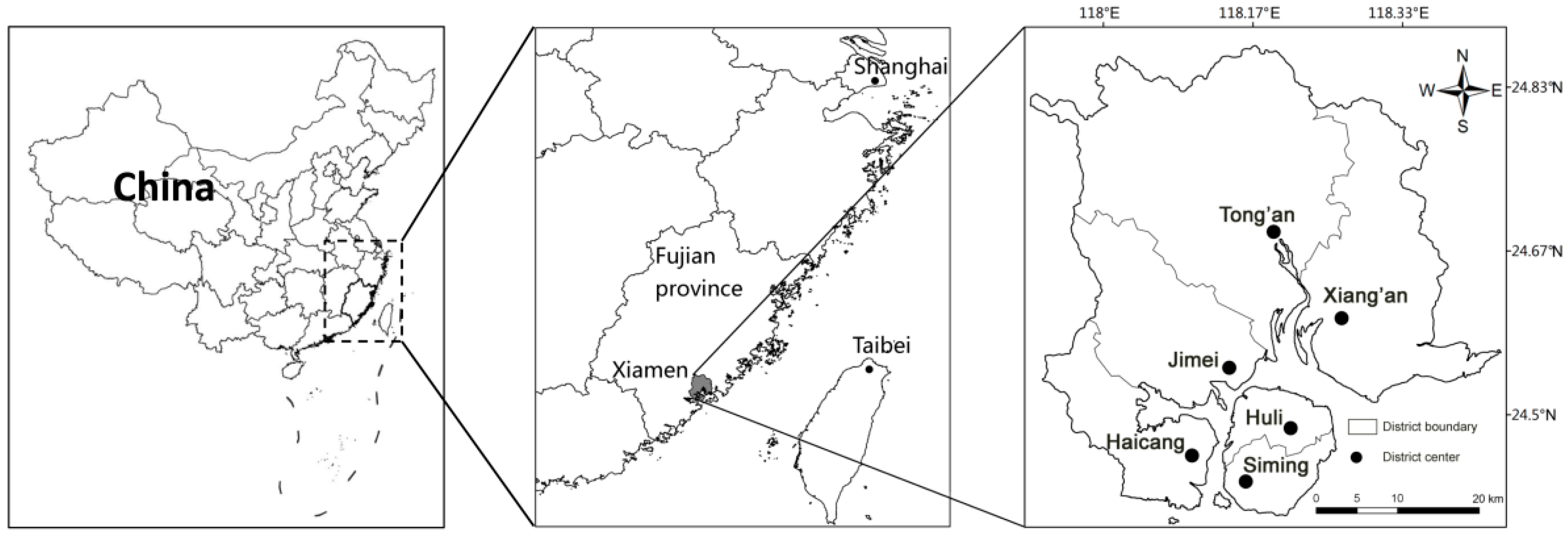
2.1. Study Area and Data Source

Xiamen, a vice-provincial city, is one of the major coastal ports in Fujian Province, China, located at latitude 24°23′ to 24°54′, longitude 117°53′ to 118°26′, in the middle of the west side of the Taiwan channel. Xiamen is a typical tourist city with beautiful port scenery. The city has jurisdiction over six administrative regions: Siming District, Huli District, Jimei District, Haicang District, Tong’an District and Xiang’an District (Figure 1). The whole city has a total administrative area of 1617 km² (including both inland and surrounding sea areas).

Xiamen’s industrialization and urbanization rate has been rapid since the establishment of the Special Economic Zone in 1980, especially in the last 30 years from 1989 to 2018. By the end of 2020, the total permanent resident population in Xiamen was 5.16 million, and the urbanization ratio reached 89.4% in 2020, far higher than the national ratio of 60.98% (Seventh National Census in 2020).

This study takes the six districts of Xiamen as the research area and 1989–2018 as the research period. The whole period was divided into three phases: 1989–2000 as Phase I, 2000–2010 as Phase II, and 2010–2018 as Phase III. For land-use analysis, 4 Landsat Thematic Mapper (TM) images (1989, 2000, 2010 and 2018) from the Chinese Academy of Sciences were taken to interpret land use/cover maps, including farmland, built-up land, watershed, grassland and forestland. The spatial resolution was 30 m, and the overall map accuracy of all land-use types exceeded 90%. ArcGIS 10 was used to conduct the analysis of land use and geographical maps. It should be noted that there are slight differences among the boundaries of the land-use map obtained from 4 images, which is mainly due to the following: (1) The coastline changes continuously under the influence of natural tides and artificial land reclamation. (2) The districts of Xiamen have experienced several changes, and the boundaries of each district were not stable until 2003. (3) In the process of land-use interpretation, there are slight deviations. Based on the land-use data, ESV was calculated and analyzed with value coefficients, as presented in the Methods section.

2.2. Methods

2.2.1. Land-Use Change

Land-Use Net Change (LUNC) in this paper is used to describe the amount of change while Land-Use Dynamic Degree (LUDD) is used to evaluate the rate of change in a given time period. The formula of these two indexes is shown in the following:

$$LUN{C}_i=L{U}_{ib}-L{U}_{ia}$$

(1)

$$LUD{D}_i=\frac{LUN{C}_i}{L{U}_{ia}}\times \frac{1}{T}$$

(2)

where LUNC_i represents the net change amount of some land type; LU_ib represents the value at the end of the study period; LU_ia represents the value at the beginning; LUDD_i represents the dynamic degree; and T represents the years of research period. Thus, the formula calculation results of LUDD_i show the annual average change rate of the land type.

As an important tool to analyze land change, the land-use transition matrix is used to measure the trend, quantity and structure characteristics of land transition, specifically to reflect the situation of land transition in a certain period. At present, the widely used transition matrix is a two-dimensional matrix shown as follows:

$$S_{ij}=\left[\begin{array}{ccc}{S}_{11}& \cdots & S_{1n}\\ ⋮& \ddots & ⋮\\ S_{n1}& \cdots & S_{nn}\end{array}\right]$$

(3)

where S represents the area; n represents the number of land-use types; i and j represent the land-use types at the beginning and end of the study period, i.e., land type i is transformed into land type j during the study period.

The transition matrix is not a calculation formula or index, but only lists the transition area between land types in the form of a matrix, which is convenient for tracking and analyzing the structure, changing direction and quantity of land types in the initial year and the final year.

2.2.2. ESV Change

In order to analyze the change of ESV, we set up an indicator of ESV contribution rate (CR) to the commonly used ESV calculation method. The CR describes how the change of a single ESV aspect to the total ESV, viz.:

$$\mathrm{ESV}=\sum V_i\times A_i$$

(4)

$${\mathrm{ESV}}_s=\sum V_{si}\times A_{si}$$

(5)

$$CR=\frac{\Delta ES{V}_s}{ESV}$$

(6)

where ESV is the total value in the study area; V_i is the ESV of land-use type i per unit area; and A_i is the area of land-use type in the study area. ESV_s is the single value of one ESV type; and V_si is the single value of ESV type of land-use type i per unit area. CR is the ratio of a single ESV type change ΔESVs to the total ESV.

Xie also claimed that there are still many important scientific problems to be solved in this method. For example, it only provides a unit price of ecosystem service value in the average state of China, which failed to consider the spatial heterogeneity of ecosystem service value. However, although other scholars already improved on this ESV method, many of them are still based on the equivalent table proposed by Xie in 2003. Thus, this evaluation system has been widely used in ESV accounting research. Considering the availability of data, the present study uses the ESV coefficient table by Xie in 2007 for calculation (

Table 1. The values per unit area of ecosystem services in China (CNY·hm⁻²·a⁻¹, 2007).

First Class Types	Second Class Types	Forestland	Grassland	Farmland	Water Area
Provisioning Service (PS)	Food production (FP)	148.2	193.1	449.1	238.0
	Raw material production (RMP)	1338.3	161.7	175.2	157.2
Regulating Service (RS)	Gas regulation (GR)	1940.1	673.7	323.4	229.0
	Climate regulation (CR)	1827.8	700.6	435.6	925.2
	Hydrological regulation (HR)	1836.8	682.6	345.8	8429.6
	Waste disposal (WD)	772.5	592.8	624.3	6669.1
Supporting Service (SS)	Soil conservation (SC)	1805.4	1006.0	660.2	184.1
	Biodiversity maintenance (BM)	2025.4	839.8	458.1	1540.4
Cultural Service (CS)	Aesthetic landscape (AL)	934.1	390.7	76.4	1994.0

), represented by the Chinese Yuan (CNY). In 2007, USD 1 approximately equaled CNY 7.6.

3. Results

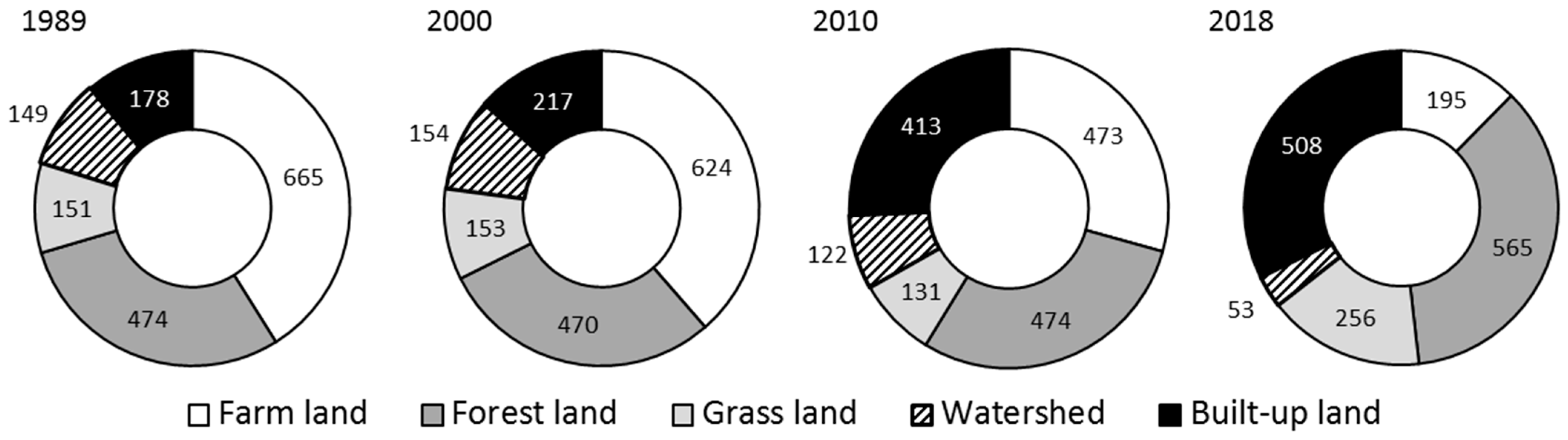
3.1. The Change of Land-Use Structure

• General situation

In the first three time nodes (1989, 2000, 2010), the total area of farmland and forestland accounted for 70.4%, 67.7% and 58.7% of the total area in Xiamen, respectively, while in 2018, forestland and built-up land accounted for the largest proportion of the land-use structure. The change of all land types during the whole period is shown in Figure 2.

For the net change amount, the ranking of all the land types in the whole period is: farmland (−470.0 km²) > built-up land (329.8 km²) > grassland (105.1 km²) > watershed (−95.5 km²) > forestland (90.6 km²). The built-up land had the largest increase from 11.0% in 1989 to 25.6% in 2010 and 32.2% in 2018, becoming one of the main land types. The top two biggest loss of the land use is the farmland and watershed, with farmland loss of 70.7% and watershed dropping from 148.9 km² (9.2%) in 1989 to 53.4 km² (3.4%) in 2018. The large reduction of farmland and watershed in the study period may be due to the occupation of farmland and the landfill of coastal watershed in the process of urbanization, especially for the development of the port industry, aquaculture industry and coastal tourism industry. However, the total amount and proportion of forestland had no big change, indicating that the forestland has been well protected in the last 30 years.

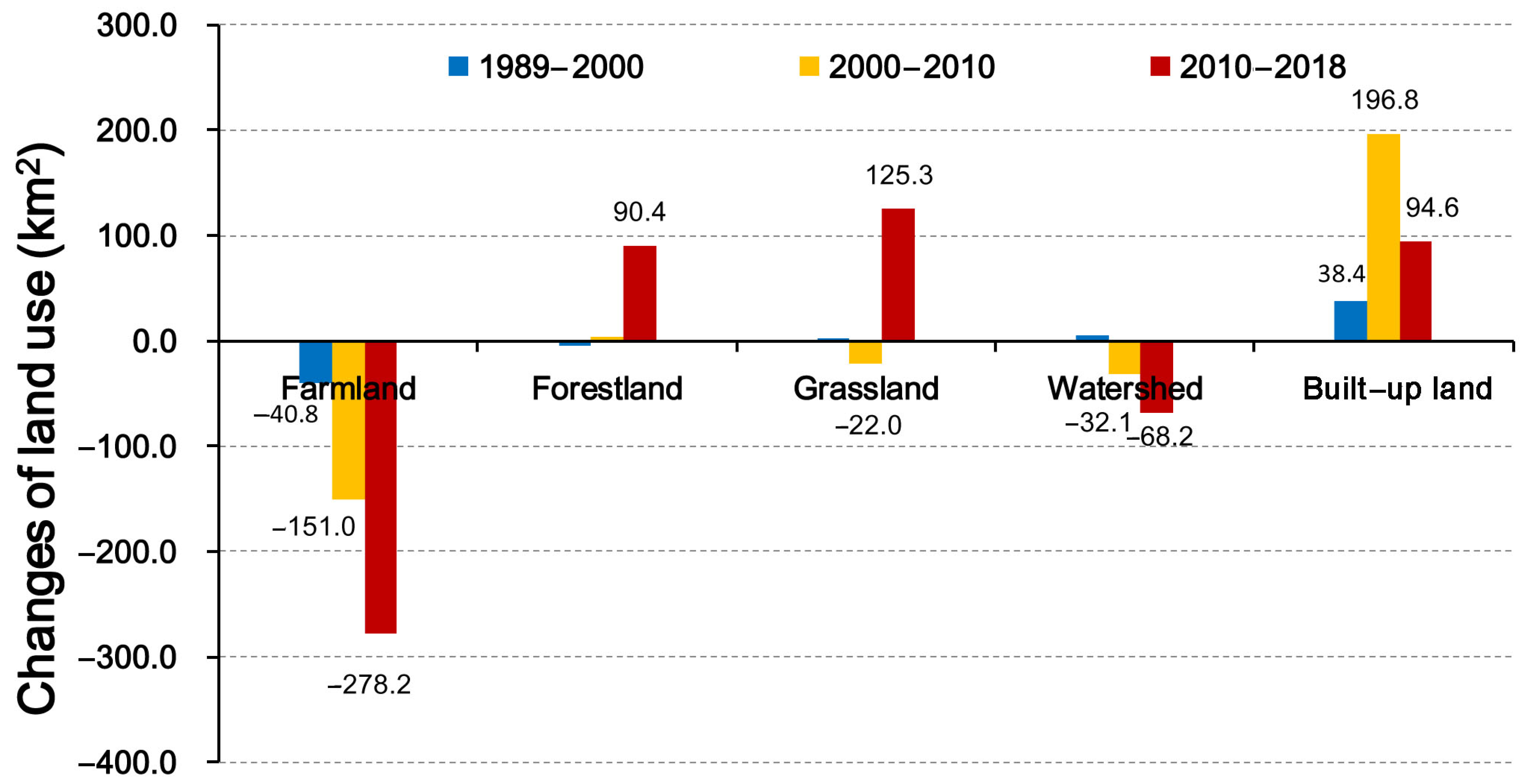
• Phase characteristics

Considering the land changes in the three time phases (Figure 3), the largest net change in Phase I (1989–2000) was the decrease of farmland (40.8 km²), followed by the increase of built-up land (38.4 km²), while the smallest change was the increase of grassland (1.8 km²) for Phase II (2000–2010). The largest net change was the increase of built-up land (196.8 km²), and the smallest was the increase of forestland (4.4 km²). Markedly, the net change of all land types in this phase was several times higher than Phase I, of which the largest was 1248.5% of grassland, and the smallest was 105.0% of forestland. For the final Phase III (2010–2018), the largest net change was the decrease of farmland (−278.2 km²), and the smallest is the decrease of watershed (−68.2 km²). Except for built-up land, the net change of other land types is still several times higher than that in Phase II, with the largest increase of 2071.7% in forestland and the smallest increase of 48.1% in built-up land (Figure 3).

The comparison of the three phases shows that the fastest growth of the built-up land in Xiamen—and thus the highest urbanization rate—occurred in Phase II, followed by Phase III. In contrast, farmland reduced the most. Land for watershed also reduced but the amount is relatively smaller. In Phase III, both forestland and grassland increased significantly. The possible reason may be that with the development of urbanization a large number of villagers moved into the urban area and abandoned the cultivation of farmland, resulting in farmland being converted to forestland and grassland.

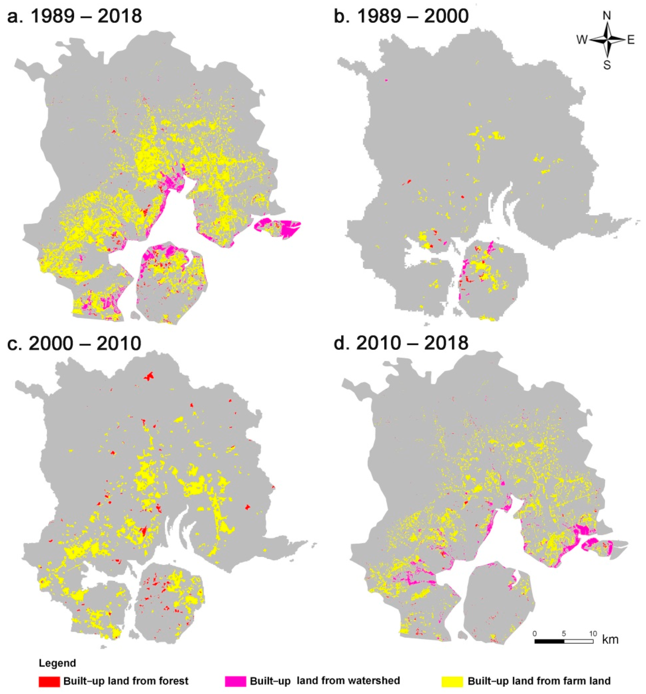
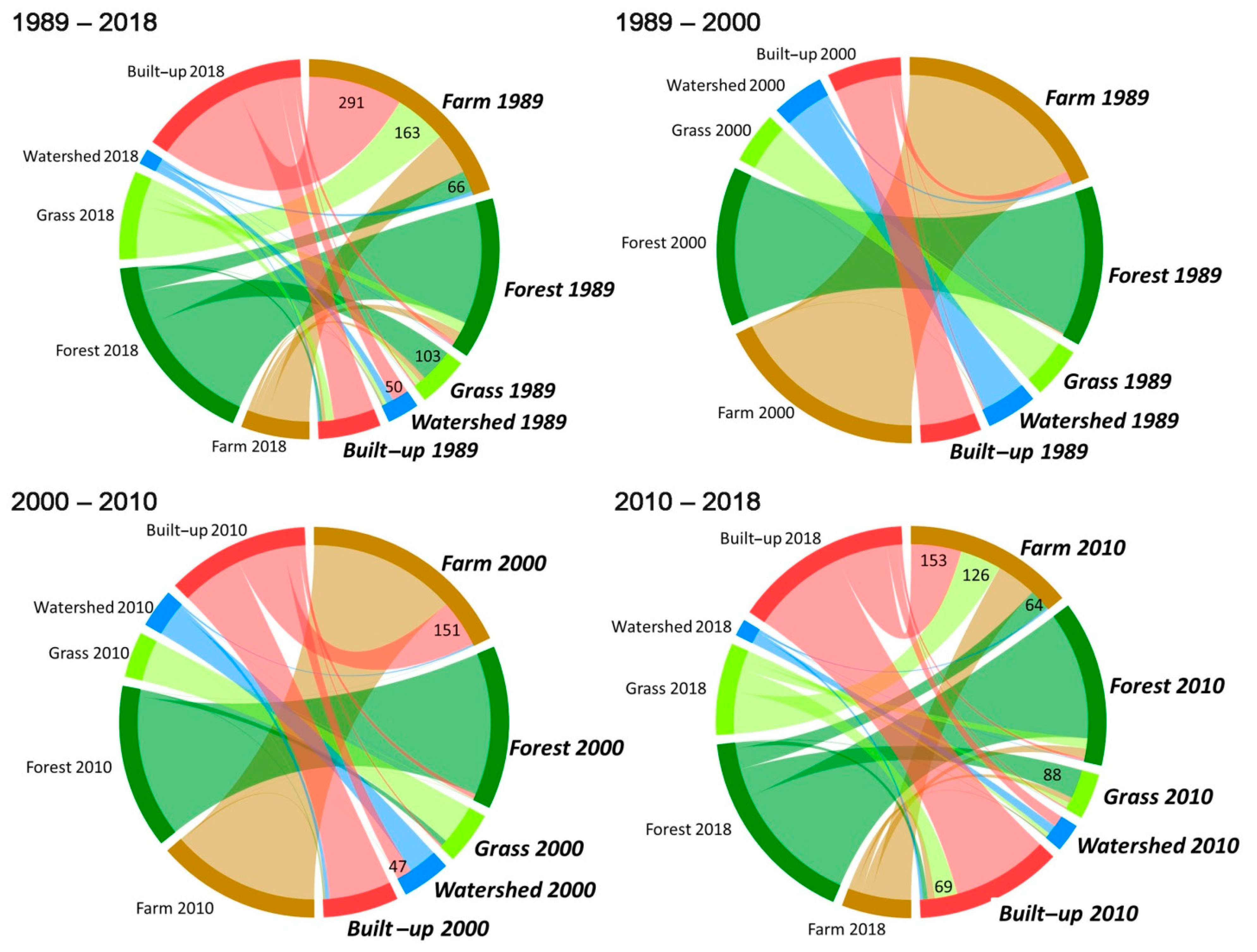
3.2. Transition of Land Use

The dynamic transition among land-use types is analyzed in ArcGIS 10. The transition information was obtained through the overlay analysis of the land-use data between two time nodes. The transfer amount over 10 km² is sorted in a land transition matrix and mapped in Figure 4.

• Spatial pattern

Figure 4 shows that the large reduction of farmland and watershed mainly occurred in coastal areas (mostly within 10 km from the coastline) and was largely converted to built-up land. The reason transition occurred in those areas may be that the coastal areas are flat and convenient for the construction of buildings, industrial parks and infrastructure. In addition, these areas are also very close to the original built-up areas, so this would naturally be impacted by local urban expansion.

• Temporal pattern of phase differences

In the whole period of study, the top three ranking of conversions with the biggest area were: farmland to built-up (291 km², 43.8% of the farmland in 1989) > farmland to grassland (163 km², 24.5% of the farmland in 1989) > grassland to forestland (103 km², 68.2% of the grassland in 1989), as shown in Figure 5 and Figure 6. Meanwhile, the urbanization rate of Xiamen based on population statistics increased from 38.7% in 1989 to 89.4% in 2020. The land-use transition and urbanization rates reflected the migration of villagers into the urban area. Farmlands were abandoned and eventually converted to forestland and grassland over time. Then, the increase in the urban population brought more demand for house land and urban area, resulting in the acceleration of farmland loss through their conversion to built-up land especially in the peri-urban areas. This kind of interactive stimulation and self-reinforcing feedback loop between urbanization and farmland loss is similar to the concept of reflexivity in social science and economics.

In Figure 5, generally, in all the three phases, the largest transition amount was from farmland to built-up land. In Phase I, it was 31.8 km² (71.3% of the total loss of farmland). In Phase II, it was 150.5 km² (96.0%), and in Phase III, it was 153.0 km² (43.8%). This means that for the whole period, farmland has been occupied due to the industrial and urbanization development. In particular, during Phase II (2000–2010), the area of built-up land increased most sharply, from 216.7 km² (13.4%) in 2000 to 413.5 km² (25.6%) in 2010, nearly double. During the same period, 47.3 km² of the newly added built-up land came from the watershed, accounting for 30.8% of the watershed loss. Large areas of farmland and watershed converted to built-up land during this rapid phase of urbanization Xiamen. Especially, the increment of built-up land significantly exceeded other land types in Phase I or the same phase. Generally, the main urbanization acceleration in Xiamen occurred in this phase, and the increasing built-up land mainly came from landfilling of watershed and farmland conversion.

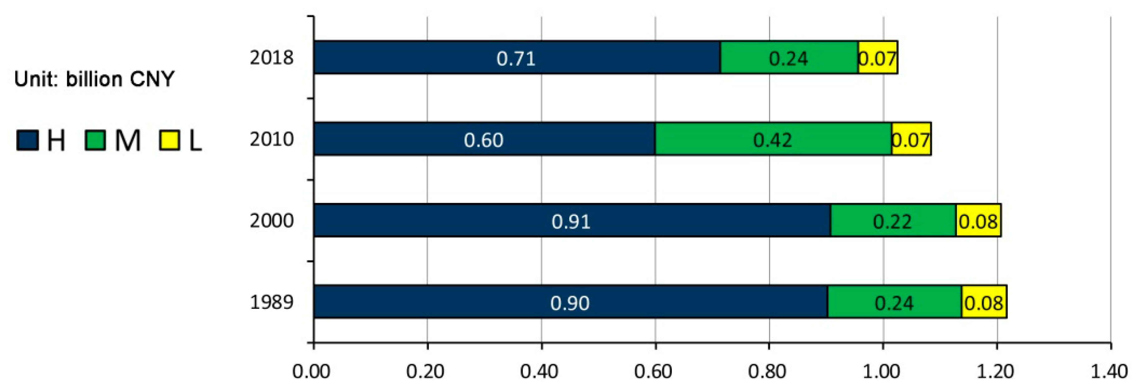
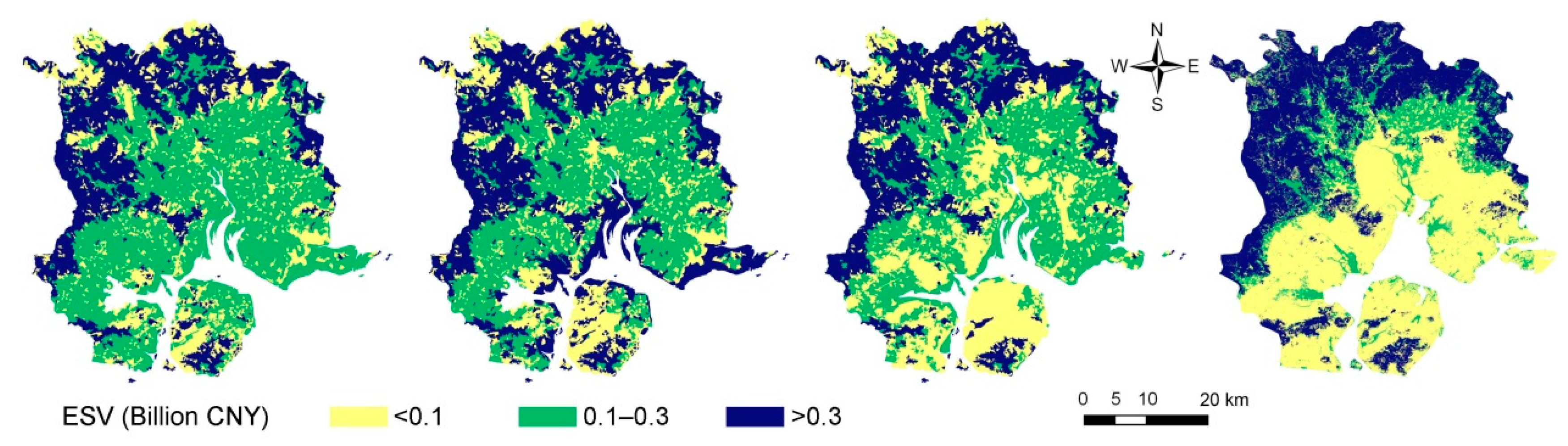
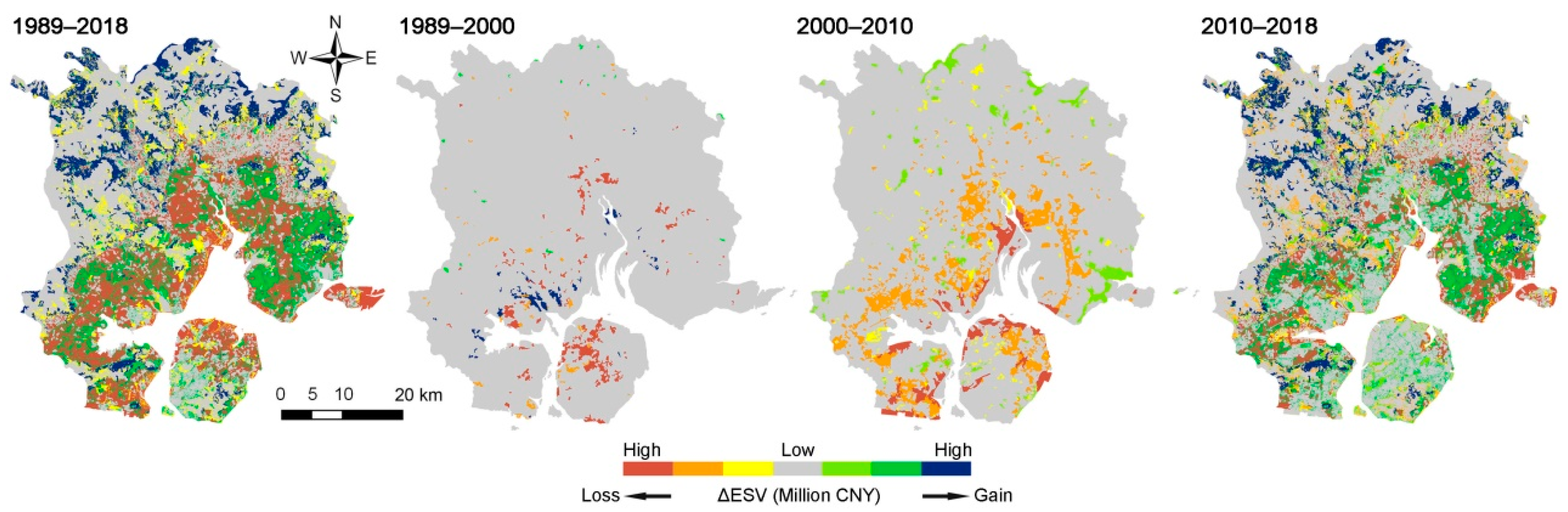
3.3. ESV Change and Spatial Distribution

In order to map the spatial distribution and observe the pattern of ESV changes, three categories of the total ESV change were considered: high-value area (CNY >0.3 billion), medium-value area (CNY 0.1–0.3 billion) and low-value area (CNY <0.1 billion). For the sub-components (PS, RS, SS and CS), the three categories were classified by hierarchical cluster. The calculated results with its H–M–L structure in Xiamen are shown in Figure 6.

The total amount of ESV in the study area was in a downward trend in the whole period, indicating the decline of the ecosystem services. In Phase I, the total amount of ESV changed slightly (CNY −10 million), but the decrease in Phase II (CNY −0.13 billion) was 1382.6% of that in Phase I, more than ten times. This is mainly due to the reduction of the high-value part, from CNY 0.91 billion in 2000 to CNY 0.6 billion in 2010. Among all the losses, the largest contribution to the total loss in this phase is the decrease of ESV from watershed (CNY −70 million, CR 34%), followed by the loss of ESV from farmland (CNY −50 million, CR 28%). As described earlier in the analysis of land-use change, the reason for such ESV loss is the rapid urbanization in this period.

Regarding the spatial distribution of ESV (Figure 7), the medium-value areas of ESV in Xiamen occupied most of the regions near the coastline in 1989, the low-value areas were very few, and the high-value areas were mainly located in the northern mountainous region. In 2000, the low-value areas had expanded on the island, mainly due to the transition of farmland into built-up land caused by urbanization. In 2010, except for the mountain areas, almost the whole island had become low-value areas, and the parts near the coastline and the original built-up areas outside the island also became mostly low-value areas. In 2018, nearly all coastal regions were of low value. Medium-value areas had been squeezed out, resulting into a more polarized ESV (Figure 7).

All the ESV components were in a downward trend from 1989 to 2018 (Figure 8). The ranking of proportion of ESV components was: RS (53.5–57.8%) > SS (25.2–28.8%) > PS (10.0–10.5%) > CS (7.0–7.3%). RS had the largest proportion and decrease which was mainly due to the large-scale conversion of watershed to built-up land in the urbanization process, resulting in loss of RS sub-components water regulation (CNY −40 million) and waste disposal (CNY −40 million). In contrast to the largest reduction of farmland, the change of PS was the smallest, with its sub-ESV component of food and raw material production not decreasing as sharply (CNY −10 million of food production and CNY −4 million of raw material production). The reason for this is that the coefficient of forest for raw material production in the ESV coefficient table is the largest (CNY·hm⁻²·a⁻¹ 1338.32), followed by farmland (CNY·hm⁻²·a⁻¹ 175.15). Thus, the forestland area in Xiamen basically remained stable (470.1 km²–474.5 km²) in the last 30 years, so the impact of the decline of farmland on PS (food and raw material production) was greatly alleviated. Considering that forestland is the main component of ESV in the study area (accounting for 49.14–55.32%), the protection of forestland in Xiamen has played a positive key role in maintaining the stability of ESV.

During the period of 2000–2010, when ESV decreased sharply (Figure 8), it is obvious that the main reason was the large reduction of RS, especially the ESV change of water regulation made the largest contribution (CR 26.39%), followed by waste disposal (CR 25.45%). There are two reasons for this: one is that the area of farmland and watershed decreased the most at this stage; the other is that the ESV coefficient of water regulation (CNY·hm⁻²·a⁻¹ 8429.61) and waste disposal (CNY·hm⁻²·a⁻¹ 6669.14) was also relatively very large.

In terms of ESV spatial distribution (Figure 9), on the first three time nodes (1989, 2000 and 2010), the high-value and medium-value of PS, RS and SS occupied large areas in the northern mountainous region, far from the coastline. While the low-value areas of PS and SS were mainly distributed in coastal areas, with clustering built-up areas and watershed with low value contributions (both area and coefficient). The low-value area of CS was widely distributed in the lowland except the forestland (high-value area) and watershed (medium-value area).

In 2018, due to the continuous reduction of farmland and watershed but substantial increase of built-up land, there was no longer any medium-value area for four sub-components, resulting in a spatial pattern of polarization between high-value areas and low-value areas (Figure 9).

These results show that, for the study area of Xiamen City, due to the large-scale transition of watershed and farmland to low ESV areas of built-up land, ecosystem service functions such as water regulation and waste disposal tended to be weakened, finally leading to the downward trend of overall ESV. Considering that forestland is the most important land for ESV, Xiamen should strengthen the protection of ecological land such as forestland, farmland and watershed in future urban planning. In addition, Xiamen should also plan to protect ecological land and promote urban greening in large-scale built-up urban areas to avoid ecological imbalance and polarization.

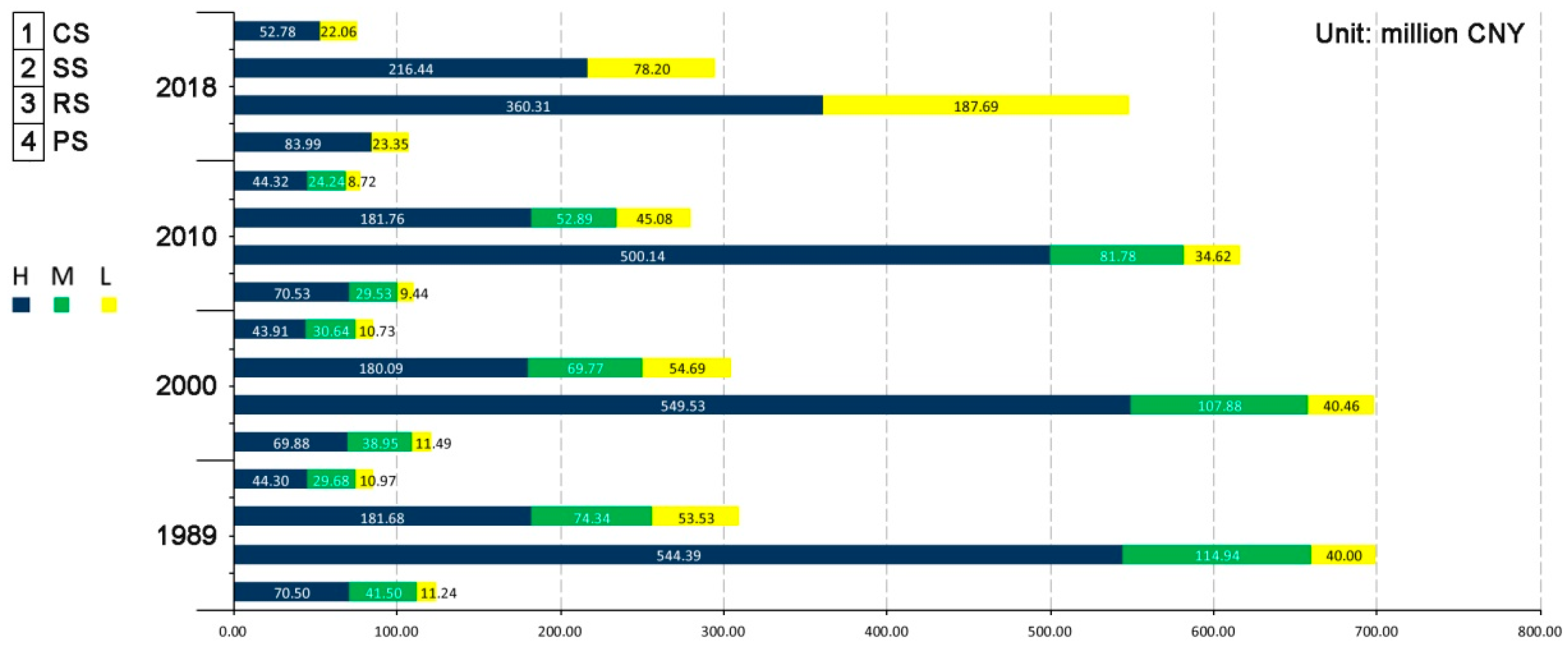
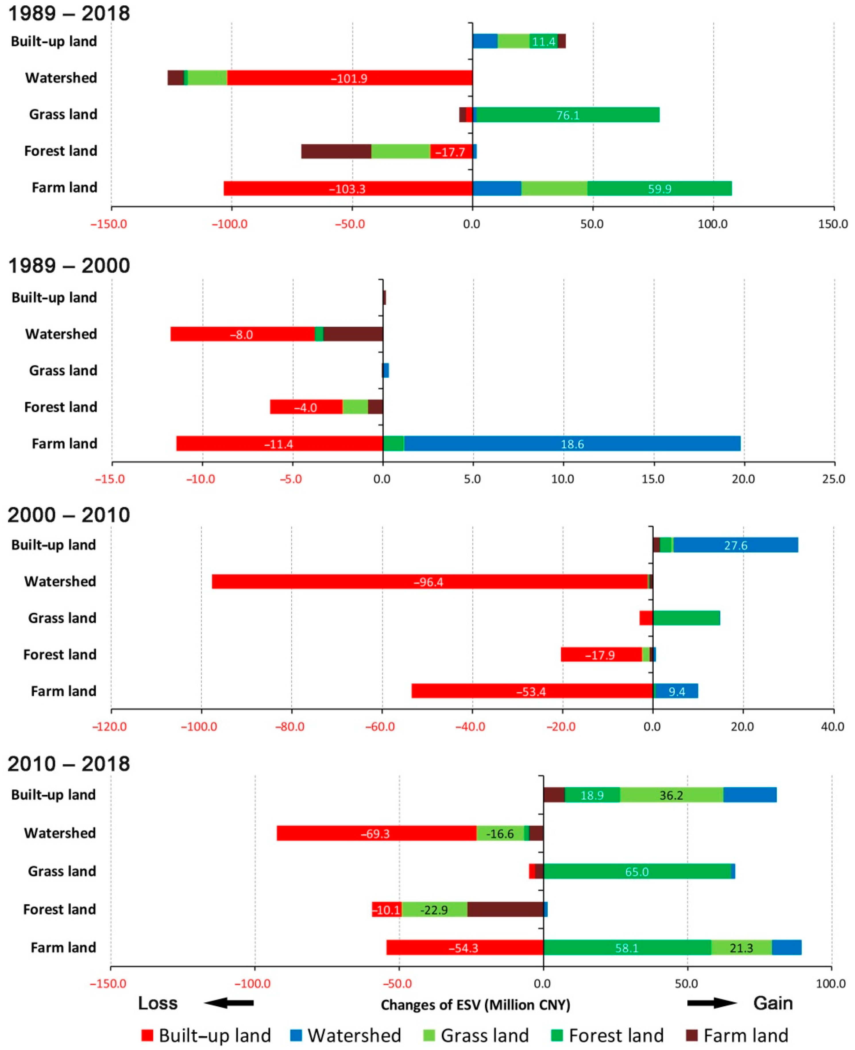
3.4. Impact of Land Use Transition on ESV

The previous analysis shows that the built-up land continued to increase while the farmland and watershed always decreased during the whole study period, resulting in the overall ESV decreasing accordingly. Focusing on the detailed amount and direction of ESV changes due to land transition, Figure 10 shows the spatial distribution of gain and loss of ESV in different phases of development.

There was a substantial reduction of ESV that mainly occurred in the coastal region where large areas of farmland and watershed converted to built-up land. The transition of farmland to built-up land reduced ESV by CNY 103.3 million, and the transition of watershed to built-up land reduced ESV by CNY 101.9 million (Figure 11). The large increase of ESV mainly occurred in the northern mountainous area due to the transition of farmland and grassland to forestland (Figure 10). The transition of farmland to forestland increased ESV by CNY 59.9 million, and the transition of watershed into built-up land reduced ESV by CNY 76.1 million (Figure 11).

There was only a slight land change in Phase I, and the corresponding change of ESV was sporadic and scattered in spatial distribution (Figure 10). The decrease of ESV was mainly due to the transition of farmland and watershed to built-up land (CNY 11.4 million of farmland and CNY 8 million of watershed, see Figure 11), occurring in the north of the island with a scaled industrial zone and newly-built residential areas (Figure 9). The increase of ESV was mainly due to the transition of off-island farmland to watershed, which may be used for aquaculture near the coast (Figure 10).

In Phase II, ESV decreased significantly, which occurred widely both inside and outside the island (Figure 10), still due to the loss of farmland and watershed to built-up land (CNY 54.2 million of farmland and CNY 96.6 million of watershed, see Figure 11). Inside the island, the transition clustered in the east and north, while outside the island it clustered near the coastline (Figure 10). These areas are adjacent to the original built-up areas of the city and would be affected by further urbanization.

In Phase III, the increase and decrease of ESV caused by land use were almost balanced (Figure 11), and the decrease of ESV was still mainly caused by transition of watershed and farmland to built-up land (CNY 69.3 million for watershed and CNY 54.3 million for farmland, see Figure 11). In the previous period, all the farmland on the island had nearly been converted to built-up land (Figure 10). Therefore, in this phase, the transition mainly occurred outside the island, especially in the coastal zone of Xiang’an District. Xiang’an District is the last one established and developed in Xiamen (Figure 10). It can be seen that the urban expansion in Xiamen has developed in nearly all the available flat land (Figure 10), while the increase of ESV was mainly caused by the transition of grassland and farmland to forestland (CNY 65.0 million from grassland, CNY 58.1 million from farmland, see Figure 11). It mainly occurred outside the island, distributed in the northern mountains (Figure 10).

The change and spatial distribution of ESV in each phase demonstrated the general situation of ESV in Xiamen. It also provides reference for land planners and managers to formulate appropriate land-use plans, as well as protection or compensation measures for the ecological environment [42]. These measures are needed to avoid adverse results such as ecological imbalance caused by the over loss and unbalance distribution of ESV.

4. Discussion

4.1. Changes in Land Use and Ecosystem Services

Investigating the conditions of land-use change and related ESV spatial pattern changes in Xiamen city at different time nodes and periods spanning 30 years, we observe that the land use and transition were very significant from 1989 to 2018. In the initial 1989–2000 period, the land-use type of Xiamen was mainly farmland and forestland, both of which were more than 450 km². In 2010, the area of farmland, built-up land and forestland was more than 400 km². In 2018, the built-up land and forestland were more than 500 km², and the farmland was less than 200 km². Thus, from 1989 to 2018, farmland continued to decrease significantly, and the built-up land increased significantly, which may be mainly caused by population growth, industrialization and urbanization [42]. The growth of a large number of industrial areas, the investment in infrastructure construction and real estate economy (including ground hardening, road and building construction), as well as the construction of new rural areas, the tourism industry, port logistics, etc., are specific reasons for the continuous increase in the area of built-up land. Under the construction of ecological civilization proposed by the government in November 2012, the growth of built-up land began to slow down from 2010 to 2018. Some built-up land was converted to other land types, grassland increased and forestland remained stable. However, from 2010 to 2018, the area of built-up land still increased by 22.9% (94.5 km²) and became the second largest area after forestland in 2018. Urbanization, population growth, and the growth of built-up land not only promote economic development, but also bring great pressure to the ecological environment and limited natural resources. The value of ecosystem services in Xiamen significantly decreased during the study period.

From 1989 to 2018, the ESV of Xiamen City decreased from CNY 1.22 billion to CNY 1.02 billion, with a total loss of CNY 0.2 billion, which is similar to the trend in Fujian province where Xiamen is located in [40]. The water area and farmland showed the largest contribution rate to the reduction of ESV in Xiamen City (a decrease of CNY 0.19 billion and CNY 0.17 billion, respectively). This is an important reason for the decline of the total ESV, just like the situation in Hangzhou Bay [41]. According to Figure 3, we can also see that it is due to the large amount of water area and farmland being converted to built-up land. Like another southern region Xishuangbanna, hydrological regulation, climate regulation, waste disposal and biodiversity are the most important ecosystem service functions in the study area [43]. However, the value of hydrological regulation and waste disposal decreased significantly from 1989 to 2018. The reason for this phenomenon is that the water area in the study area was converted to built-up land, resulting in a significant increase in the built-up land area and a significant decrease in the water area.

In addition to the significant decline in the total amount of ESV and the related threat to urban ecological security, the obvious trend of spatial polarization of ESV is another great risk to sustainable development in Xiamen. As the terrain of Xiamen is high in the west and low in the east, mountains and forests are mainly located in the northern area, while the southern region is flat and contains most of the built-up land, farmland and coastal water area. In the rapid urbanization, a large number of water areas and farmlands in the southern flat region were converted to built-up land, which has significantly reduced the ESV. This change trend causes the spatial distribution of ESV in Xiamen to become increasingly unbalanced and polarized, with high-value areas decreased and low value increased [39,43]. In 2018, there were few medium-value areas of ESV. Meanwhile, the high-value areas were mainly distributed in the northern mountainous areas, with the low-value areas concentrated in the flat areas near the coastline. The spatial distribution of high, medium and low value areas is now very unbalanced, with the medium value areas disappearing. This situation will aggravate urban challenges such as the heat island effect, traffic congestion, housing tension, environmental pollution, and lack of urban greening.

To sum up, the rapid economic development and urbanization in Xiamen has led to built-up land growth at the cost of reducing the ecological spaces associated with water areas and farmland. This is now posing significant challenges in the city’s efforts towards eco-environment protection and urban sustainable development.

4.2. Limitations and Future Work

In the evaluation of ESV, in addition to the area change, the correction and determination of the equivalent value have a great impact on the ESV. In this paper, the equivalent factor method was used to evaluate the ESV, which is conducive to the comparison between different regions. However, the equivalent factor method is more dependent on the equivalent value of the assessment, and different assessment methods may cause large differences in the results. In this study, the water area contributes a larger ESV change with a smaller area proportion, which indicates that the water area has important value significance for the ESV of Xiamen but also shows that the equivalent value has a great impact on the ESV.

In the spatial analysis of the study area, this paper mapped the spatial difference of ESV and its relationship with the land use by means of high, medium and low category analysis, so as to demonstrate the spatial pattern and temporal evolution of ESV in Xiamen. However, this paper does not take the smaller administrative units (counties, districts and towns) within the study area as the statistical unit to evaluate and analyze the spatial difference of ESV. At the same time, correcting the difference of equivalent value in Xiamen and time series will help make the calculation results closer to the actual value and improve the accuracy.

In addition, further study could explore the ESV sensitivity to land-use changes and the correlation between them [37]. Analysis of future land-use planning scenarios could be conducted to optimize the spatial balance of ecosystem services. Particularly, setting green infrastructure in urban core areas, such as in Xiamen island, might help to decrease the polarization [46,47]. Using cellular automata to simulate future land-use planning and explore settings for ESV optimization could help identify viable urban sustainable development options [11,12].

5. Conclusions

We analyzed the spatiotemporal characteristics of land-use evolution in the coastal city of Xiamen from 1989 to 2018, covering the early years of its industrialization to the rapid urbanization that has led to the modern city that it has become today, and showed that its overall ESV has significantly declined and become more polarized between high-value and low-value land areas.

For the whole study period, the built-up land grew rapidly, mainly because of the conversion of farmland and landfill of the watershed to accommodate the growing urban population. The most intense period of change was Phase II (the 2000–2010 period). The land changes in Phase I were relatively mild and in Phase III were huge but not as intense as those during Phase II.

The rapid economic development and urban expansion reflected in these land changes over these time periods, translated to the decline of the total amount of ESV in Xiamen, with the decline in Phase II being much higher than that in other phases. The biggest contribution to the reduction of ESV in this phase was the loss of watershed (CNY −70 million), followed by the loss of farmland (CNY −50 million). In 2018, there were few medium-value areas of ESV. Meanwhile, the high-value areas were mainly distributed in the northern mountainous areas, with the low-value areas concentrated in the flat areas near the coastline. The spatial distribution of high, medium and low value areas is now very unbalanced, with the medium value areas disappearing.

The ESV components that changed most are ranked as follows: RS > SS > PS > CS. The significant reduction of RS was mainly due to the loss of water areas to low ESV areas (built-up land), leading to the weakening of ecosystem service functions such as water regulation and waste disposal.

Rapid urbanization and built-up land growth at the cost of occupying the ecological space of water area and farmland is an important obstacle to the eco-environment protection and urban sustainable development in Xiamen. This situation will aggravate urban challenges such as the heat island effect, traffic congestion, housing tension, environmental pollution and lack of urban greening. Therefore, Xiamen should strengthen the protection of ecological land such as forestland, farmland and watershed in future urban planning and development policy or plan ecological land in large-scale built-up areas as ESV compensation and encourage measures to avoid over-development, ecological imbalance and polarization.

The Xiamen case study provides lessons and reference for land planners and managers in other parts of China to formulate appropriate land-use plans, as well as protection or measures for the ecological environment. Other cities in the world facing opportunities—or challenges—of rapid urbanization and industrialization also need to pay attention to the potential problems such as ecological imbalance and ESV reduction caused by land-use change. In these types of research, understanding the spatial distribution of ESV and its temporal evolution would help policy makers avoid or minimize ecological imbalance through appropriate land-use planning. The potential ESV impacts of future land-use changes can be further explored by simulation—for example, by cellular automata—to support regional and urban sustainable development.

References

1. Sterling, S.M.; Ducharne, A.; Polcher, J. The impact of global land-cover change on the terrestrial water cycle. Nat. Clim. Chang. 2012, 3, 385–390. [Google Scholar] [CrossRef]
2. Estoque, R.C.; Murayama, Y. Examining the potential impact of land use/cover changes on the ecosystem services of Baguio city, the Philippines: A scenario–based analysis. Appl. Geogr. 2012, 35, 316–326. [Google Scholar] [CrossRef]
3. Costanza, R.; D’Arge, R.; Groot, R.D.; Farber, S.; Grasso, M.; Hannon, B.; Limburg, K.; Naeem, S.; O’Neill, R.V.; Paruelo, J.; et al. The value of the world’s ecosystem services and natural capital. Nature 1997, 387, 253–260. [Google Scholar] [CrossRef]
4. Costanza, R.; Groot, R.D.; Sutton, P.; Ploeg, S.V.D.; Anderson, S.J.; Kubiszewski, I.; Farber, S.; Turner, R.K. Changes in the global value of ecosystem services. Glob. Environ. Chang. 2014, 26, 152–158. [Google Scholar] [CrossRef]
5. Ridding, L.E.; Redhead, J.W.; Oliver, T.H.; Schmucki, R.; McGinlay, J.; Graves, A.R.; Morris, J.; Bradbury, R.B.; King, H.; Bullock, J.M. The importance of landscape characteristics for the delivery of cultural ecosystem services. J. Environ. Manag. 2018, 206 (Suppl. C), 1145–1154. [Google Scholar] [CrossRef] [Green Version]
6. Stefanidis, S.; Alexandridis, V.; Mallinis, G. A cloud-based mapping approach for assessing spatiotemporal changes in erosion dynamics due to biotic and abiotic disturbances in a Mediterranean Peri-Urban forest. Catena 2022, 218, 106564. [Google Scholar] [CrossRef]
7. Song, W.; Deng, X.; Yuan, Y.; Wang, Z.; Li, Z. Impacts of land-use change on valued ecosystem service in rapidly urbanized north china plain. Ecol. Model. 2015, 318, 245–253. [Google Scholar] [CrossRef]
8. Gascoigne, W.R.; Hoag, D.; Koontz, L.; Tangen, B.A.; Shaffer, T.L.; Gleason, R.A. Valuing ecosystem and economic services across land-use scenarios in the Prairie Pothole Region of the Dakotas, USA. Ecol. Econ. 2011, 70, 1715–1725. [Google Scholar] [CrossRef]
9. Hasan, S.S.; Zhen, L.; Miah, M.G.; Ahamed, T.; Samie, A. Impact of land use change on ecosystem services: A review. Environ. Dev. 2020, 34, 100527. [Google Scholar] [CrossRef]
10. Andersson, E.; Tengö, M.; Mcphearson, T.; Kremer, P. Cultural ecosystem services as a gateway for improving urban sustainability. Ecosyst. Serv. 2015, 12, 165–168. [Google Scholar] [CrossRef]
11. Akhtar, M.; Zhao, Y.; Gao, G.L.; Gulzar, Q.; Samie, A. Assessment of ecosystem services value in response to prevailing and future land use/cover changes in lahore, pakistan. Reg. Sustain. 2020, 1, 11. [Google Scholar] [CrossRef]
12. Lyu, R.; Zhang, J.M.; Xu, M.Q.; Li, J.J. Impacts of urbanization on ecosystem services and their temporal relations: A case study in Northern Ningxia, China. Land Use Policy 2018, 77, 163–173. [Google Scholar] [CrossRef]
13. Costanza, R.; Groot, R.D.; Braat, L.; Kubiszewski, I.; Grasso, M. Twenty years of ecosystem services: How far have we come and how far do we still need to go? Ecosyst. Serv. 2017, 28, 1–16. [Google Scholar] [CrossRef]
14. Rönnbäck, P. The ecological basis for economic value of seafood production supported by mangrove ecosystems. Ecol. Econ. 1999, 29, 235–252. [Google Scholar] [CrossRef]
15. Polasky, S.; Nelson, E.; Pennington, D.; Johnson, K.A. The impact of land-use change on ecosystem services, biodiversity and returns to landowners: A case study in the state of Minnesota. Environ. Resour. Econ. 2011, 48, 219–242. [Google Scholar] [CrossRef]
16. Kozak, J.; Lant, C.; Shaikh, S.; Wang, G.X. The geography of ecosystem service value: The case of the des Plaines and Cache River Wetlands, Illinois. Appl. Geogr. 2011, 31, 303–311. [Google Scholar] [CrossRef]
17. Xie, G.; Zhen, L.; Lu, C.; Xiao, Y.; Chen, C. Expert knowledge based valuation method of ecosystem services in China. J. Nat. Resour. 2008, 23, 911–919. (In Chinese) [Google Scholar]
18. Jiang, L.; Deng, X.; Seto, K.C. The impact of urban expansion on agricultural land use intensity in China. Land Use Policy 2013, 35, 33–39. [Google Scholar] [CrossRef]
19. Wu, F. Land financialization and the financing of urban development in China. Land Use Policy 2019, 112, 104412. [Google Scholar] [CrossRef]
20. Jiao, L. Urban land density function: A new method to characterize urban expansion. Landsc. Urban Plan. 2015, 139, 26–39. [Google Scholar] [CrossRef]
21. Liu, J.Y.; Zhang, Z.X.; Xu, X.L. Spatial patterns and driving factors of land use change in China during the early 21st century. J. Geogr. Sci. 2010, 20, 483–494. [Google Scholar] [CrossRef]
22. Hui, E.C.M.; Wu, Y.Z.; Deng, L.J.; Zheng, B.B. Analysis on coupling relationship of urban scale and intensive use of land in China. Cities 2015, 42, 63–69. [Google Scholar] [CrossRef]
23. Elmqvist, T.; Fragkias, M.; Goodness, J.; Güneralp, B.; Marcotullio, P.J.; McDonald, R.I.; Parnell, S.; Schewenius, M.; Sendstad, M.; Seto, K.C.; et al. Urbanization, Biodiversity and Ecosystem Services: Challenges and Opportunities. A Global Assessment; Springer Open: London, UK, 2013. [Google Scholar]
24. Li, G.; Fang, C.; Wang, S. Exploring spatiotemporal changes in ecosystem-service values and hotspots in China. Sci. Total Environ. 2016, 545, 609–620. [Google Scholar] [CrossRef] [PubMed]
25. Xie, G.; Zhang, C.; Zhen, L.; Zhang, L. Dynamic changes in the value of China’s ecosystem services. Ecosyst. Serv. 2017, 26, 146–154. [Google Scholar] [CrossRef]
26. Long, H.; Liu, Y.; Hou, X.; Li, T.; Li, Y. Effects of land use transitions due to rapid urbanization on ecosystem services: Implications for urban planning in the new developing area of China. Habitat Int. 2014, 44, 536–544. [Google Scholar] [CrossRef]
27. Su, S.; Li, D.; Hu, Y.N.; Xiao, R.; Zhang, Y. Spatially non-stationary response of ecosystem service value changes to urbanization in Shanghai, China. Ecol. Indic. 2014, 45, 332–339. [Google Scholar] [CrossRef]
28. Ye, Y.; Bryan, B.A.; Zhang, J.; Connor, J.D.; Chen, L.; Qin, Z.; He, M. Changes in land-use and ecosystem services in the Guangzhou-Foshan Metropolitan Area, China from 1990 to 2010: Implications for sustainability under rapid urbanization. Ecol. Indic. 2018, 93, 930–941. [Google Scholar] [CrossRef]
29. Zhao, Y.; Liu, Z.; Wu, J. Grassland ecosystem services: A systematic review of research advances and future directions. Landsc. Ecol. 2020, 35, 793–814. [Google Scholar] [CrossRef]
30. Hu, Z.; Shi, H.; Cheng, K.; Wang, Y.P.; Piao, S.; Li, Y.; Zhang, L.; Xia, J.; Zhou, L.; Yuan, W. Joint structural and physiological control on the inter annual variation in productivity in a temperate grassland: A data-model comparison. Glob. Chang. Biol. 2018, 24, 2965–2979. [Google Scholar] [CrossRef]
31. Qiang, X.; Dan, H.; Yang, X. Assessing changes in soil conserved ecosystem services and causal factors in the Three Gorges Reservoir region of China. J. Clean. Prod. 2016, 163, 172–180. [Google Scholar]
32. Xie, G.; Zhang, C.; Zhang, C.; Xiao, Y.; Lu, C.X. The value of ecosystem services in China. J. Nat. Resour. 2015, 37, 1740–1746. (In Chinese) [Google Scholar]
33. Xie, G.; Zhang, C.; Zhang, L.; Chen, W.; Li, S. Improvement of the Evaluation Method for Ecosystem Service Value Based on Per Unit Area. J. Nat. Resour. 2015, 30, 1243–1254. (In Chinese) [Google Scholar]
34. Fu, B.; Shuai, W.; Su, C.; Forsius, M. Linking ecosystem processes and ecosystem services. Curr. Opin. Environ. Sustain. 2013, 5, 4–10. [Google Scholar] [CrossRef]
35. Fang, X.; Zhao, W.; Fu, B.; Ding, J. Landscape service capability, landscape service flow and landscape service demand: A new framework for landscape services and its use for landscape sustainability assessment. Prog. Phys. Geogr. 2015, 39, 817–836. [Google Scholar] [CrossRef]
36. Shi, L.; Halik, Ü.; Mamat, Z.; Wei, Z.C. Spatio⁃temporal variation of ecosystem services value in the Northern Tianshan Mountain Economic zone from 1980 to 2030. PeerJ 2020, 8, e9582. [Google Scholar] [CrossRef]
37. Sannigrahi, S.; Bhatt, S.; Rahmat, S.; Paul, S.K.; Sen, S. Estimating global ecosystem service values and its response to land surface dynamics during 1995–2015. J. Environ. Manag. 2018, 223, 115–131. [Google Scholar] [CrossRef]
38. Tan, Z.; Guan, Q.; Lin, J.; Yang, L.; Luo, H.; Ma, Y.; Tian, J.; Wang, Q.Z.; Wang, N. The response and simulation of ecosystem services value to land use/land cover in an oasis, northwest china. Ecol. Indic. 2020, 118, 106711. [Google Scholar] [CrossRef]
39. Zhang, F.; Yushanjiang, A.; Jing, Y. Assessing and predicting changes of the ecosystem service values based on land use/cover change in ebinur lake wetland national nature reserve, Xinjiang, China. Sci. Total Environ. 2019, 656, 1133–1144. [Google Scholar] [CrossRef]
40. Su, K.; Wei, D.Z.; Lin, W.X. Evaluation of ecosystem services value and its implications for policy making in China—A case study of Fujian province. Ecol. Indic. 2020, 108, 105752. [Google Scholar] [CrossRef]
41. Lin, W.; Xu, D.; Guo, P.; Wang, D.; Gao, J. Exploring variations of ecosystem service value in Hangzhou bay wetland, eastern china. Ecosyst. Serv. 2019, 37, 100944. [Google Scholar] [CrossRef]
42. Bryan, B.A.; Ye, Y.Q.; Zhang, J.E.; Connor, J.D. Land-use change impacts on ecosystem services value: Incorporating the scarcity effects of supply and demand dynamics. Ecosyst. Serv. 2018, 32, 144–157. [Google Scholar] [CrossRef]
43. Hu, Z.N.; Yang, X.; Yang, J.J.; Yuan, J.; Zhang, Z.Y. Linking landscape pattern, ecosystem service value, and human well-being in Xishuangbanna, southwest china: Insights from a coupling coordination model. Glob. Ecol. Conserv. 2021, 27, e01583. [Google Scholar] [CrossRef]
44. Tang, L.; Zhao, Y.; Yin, K.; Zhao, J. Xiamen. Cities 2013, 31, 615–624. [Google Scholar] [CrossRef]
45. Zhao, J.; Dai, D.; Lin, T.; Tang, L. Rapid urbanisation, ecological effects and sustainable city construction in Xiamen. Int. J. Sustain. Dev. World Ecol. 2010, 17, 271–272. [Google Scholar] [CrossRef]
46. Hardin, P.J.; Jensen, R.R. The effect of urban leaf area on summertime urban surface kinetic temperatures: A Terre Haute case study. Urban For. Urban Green. 2007, 6, 63–72. [Google Scholar] [CrossRef]
47. Chiesura, A. The role of urban parks for the sustainable city. Landsc. Urban Plan. 2004, 68, 129–138. [Google Scholar] [CrossRef]
Figure 1. Location of the study area of Xiamen city and its 6 districts.
Sustainability 14 12532 g001
Figure 2. The structure and proportion change of land use in Xiamen from 1989 to 2018 (km2).
Sustainability 14 12532 g002
Figure 3. The change of land use in the three phases (km2).
Sustainability 14 12532 g003
Figure 4. The spatial distribution of land-use transition in different phases: (a) for the whole period from 1989 to 2018; (b) for Phase I from 1989 to 2000; (c) for Phase II from 2000 to 2010; (d) for Phase III from 2010 to 2018. Note that due to multiple influences, especially the natural tides and artificial land reclamation, there are slight differences among the boundaries in the four time nodes.
Sustainability 14 12532 g004
Figure 5. The land-use transition among each land type in different phases of development in Xiamen (Note: considering there is inflow and outflow for all land-use types in each period, the data of 1989–2018 come from the overlay analysis between land-use data of 1989 and 2018 directly and are not based on the cumulative calculation of the three periods).
Sustainability 14 12532 g005
Figure 6. The change of total ESV and its H–M–L structure in the four time nodes, H = High-value, M = Medium-value, L = Low-value.
Sustainability 14 12532 g006
Figure 7. The spatial distribution of ESV H–M–L structure from 1989 to 2018, H = High-value, M = Medium-value, L = Low-value. Note that due to multiple influences, especially the natural tides and artificial land reclamation, there are slight differences among the boundaries in the four time nodes.
Sustainability 14 12532 g007
Figure 8. ESV sub-components and their H–M–L structure from 1989 to 2018.
Sustainability 14 12532 g008
Figure 9. The spatial distribution of 4 sub-categories of ESV from 1989 to 2018, H = High-value, M = Medium-value, L = Low-value. Note that due to multiple influences, especially the natural tides and artificial land reclamation, there are slight differences among the boundaries in the four time nodes.
Sustainability 14 12532 g009
Figure 10. The spatial distribution of gain and loss of ESV in different phases. Note that due to multiple influences, especially the natural tides and artificial land reclamation, there are slight differences among the boundaries in the four time nodes.
Sustainability 14 12532 g010
Figure 11. The gain and loss of ESV due to the transition of land use among each other in different phases.
Sustainability 14 12532 g011