An Improved Mayfly Method to Solve Distributed Flexible Job Shop Scheduling Problem under Dual Resource Constraints

Abstract

Aiming at the distributed flexible job shop scheduling problem under dual resource constraints considering the influence of workpiece transportation time between factories and machines, a distributed flexible job shop scheduling problem (DFJSP) model with the optimization goal of minimizing completion time is established, and an improved mayfly algorithm (IMA) is proposed to solve it. Firstly, the mayfly position vector is discrete mapped to make it applicable to the scheduling problem. Secondly, three-layer coding rules of process, worker, and machine is adopted, in which the factory selection is reflected by machine number according to the characteristics of the model, and a hybrid initialization strategy is designed to improve the population quality and diversity. Thirdly, an active time window decoding strategy considering transportation time is designed for the worker–machine idle time window to improve the local optimization performance of the algorithm. In addition, the improved crossover and mutation operators is designed to expand the global search range of the algorithm. Finally, through simulation experiments, the results of various algorithms are compared to verify the effectiveness of the proposed algorithm for isomorphism and isomerism factories instances.

1. Introduction

Economic globalization and the rapid development of new technologies such as cloud computing, big data, and the Internet of Things are leading the manufacturing industry to the modes of production globalization, cloud manufacturing, and intelligent manufacturing [1,2,3,4]. The traditional centralized manufacturing mode can no longer meet the fierce market competition and diversified customer needs. A large number of enterprises expand their production to the distributed production environment. Through the rational allocation, optimal combination, and sharing of resources of enterprises or factories in different regions, they can quickly improve production efficiency and quality and reduce costs and risks [5,6]. Providing reasonable and efficient resource allocation and scheduling services for collaborative production of distributed factories is a research hotspot in the field of scheduling.

The distributed flexible job shop scheduling problem (DFJSP) has many constraints and is challenging to solve. It is a more complex NP-Hard problem which has attracted the attention of many scholars at home and abroad in recent years. De Giovanni et al. [7] proposed an improved genetic algorithm to solve DFJSP with multiple flexible manufacturing units, which extended the decoding of FJSP to include the information of FMU allocation and used a new local search operator to improve the population quality. Ziaee [8] assume that the job shop of each factory/unit is configured as a flexible job shop; in order to obtain a high-quality scheduling plan quickly, a fast heuristic algorithm based on the constructive process was proposed for DFJSP. Sang et al. [9] built a DFJSP model for collaborative manufacturing of smart factories, proposed a high-dimensional multi-objective memory algorithm combing with improved NSGA-III and local search methods, and optimized economic indicators and green indicators. Xu et al. [10] proposed a three-layer coding of hybrid genetic tabu search algorithm to optimize the completion time, cost, quality, and carbon emissions of DFJSP considering outsourcing some workpieces. Meng et al. [11] proposed four MILP models and a constraint programming (CP) model for DFJSP and verified the effectiveness and superiority of the model through small and large instances. The above studies usually assume that a workpiece can be processed in only one factory. In recent years, some scholars have studied the open shop scheduling environment considering that a workpiece can be processed in different factories. Luo et al. [12] established a DFJSP mathematical model considering the workpiece transfer with the optimization objectives of the completion time, factory load, and energy consumption, and designed the GLS initialization method and a variety of neighborhood structures to improve the memetic algorithm for solving it. Gong et al. [13] considered that workpieces can be transferred between machines, job shops, and factories; studied the distributed production scheduling of different factories and job shops; and proposed a new memetic algorithm to optimize the problem’s completion time and total energy consumption. Du et al. [14] established a MILP model of dual-objective DFJSP considering the constraints of crane transportation and energy consumption and proposed an EDA-VNS hybrid algorithm to solve it. However, there is still lack of relevant literature on the transportation time required for workpiece transfer.

In addition, most studies on DFJSP consider only the constraints of machinery and equipment but ignore the constraint of worker resources that is inseparable from production scheduling. There are some related studies on FJSP in the integrated manufacturing environment. Meng et al. [15] studied the dual resource-constrained flexible job shop scheduling problem (DRCFJSP) with energy consumption awareness, proposed two MILP models, and designed a neighborhood search algorithm with eight neighborhood structures for the solution. Obimuyiwa [16] considered a limited number of cross-trained skilled installation operators, established a detailed MILP model of DRCFJSP, and solved it with a genetic algorithm. Gong et al. [17] proposed a DRCFJSP model considering workers’ flexibility and proposed a hybrid artificial bee colony algorithm to solve it.

Previously, our research group studied DRCFJSP of integrated manufacturing mode which better solved the differences of the operation levels of workers but ignored the influence of transportation time in the model established [18]. Therefore, to further study the distributed manufacturing mode scheduling problem, this paper considers the influence of worker–machine dual resource constraints and workpiece transportation time and constructs a distributed flexible job shop scheduling problem under dual resource constraints (DFJSPD) model with the completion time as the optimization objective. In addition, an improved mayfly algorithm (IMA) is proposed according to the characteristic of the model, where discrete mapping of mayfly position variables, a new three-layer coding method for multiple resource constraints, a mixed initialization strategy, an active time window decoding algorithm for idle time window, and the improved crossover and mutation modes are designed to improve solving performance of the algorithm. Finally, the experimental results show that the proposed DFJSPD model is more in line with the actual scheduling situation and the effectiveness and superiority of the improved algorithm.

The remainder of this work is organized as follows. Section 2 establishes the DFJSP model and Section 3 gives the improved mayfly solution. Experimental analysis and results are presented in Section 4. Section 5 concludes the main findings.

2. DFJSPD Modeling

2.1. DFJSPD Problem Description

DFJSPD is described as: $n$ workpieces $J_i\left(i=1,2,\dots ,n\right)$ needs to be processed in $F$ flexible job shop type factories $F_f\left(f=1,2,\dots ,F\right)$. The workpiece $i$ has $n_i$ processes with priority constraints among them. In the factory $F_f$, there are $m_f$ machines $M_{fk}\left(k=1,2,\dots ,m_f\right)$ and $w_f$ workers $W_{fs}\left(s=1,2,\dots ,w_f\right)$ operating the machines, generally $m_f>w_f$. The machines in the factory include CNC machines and non-CNC machines. The workers are responsible for the preparation including the loading and unloading, the replacement of tool fixtures and cleaning of CNC machines, and the preparation and machining of non-CNC machines. Individual differences among workers lead to the differences of operation efficiency. The basic times of preparation and machining on different machines are known. Workpieces are transported between machines in a factory or different factories with known transportation time. DFJSPD can be divided into four sub-problems: factory selection, machine selection, worker selection, and process sequencing.

Considering the data in

Table 1. An example of DFJSPD.

Workpiece	Process	${\mathit{F}}_1$			${\mathit{F}}_2$			Workpiece	Process	${\mathit{F}}_1$			${\mathit{F}}_2$
		${\mathit{M}}_1^{\ast }$	${\mathit{M}}_2^{\ast }$	${\mathit{M}}_3$	${\mathit{M}}_4$	${\mathit{M}}_5$	${\mathit{M}}_6^{\ast }$			${\mathit{M}}_1^{\ast }$	${\mathit{M}}_2^{\ast }$	${\mathit{M}}_3$	${\mathit{M}}_4$	${\mathit{M}}_5$	${\mathit{M}}_6^{\ast }$
$J_1$	$O_{11}$	1/3	2/5	-	2/4	-	1/3	$J_3$	$O_{31}$	-	2/4	1/3	2/5	-	3/7
	$O_{12}$	1/2	-	2/4	2/4	1/3	-		$O_{32}$	3/6	-	2/4	-	1/3	2/4
$J_2$	$O_{21}$	-	2/5	3/7	-	2/4	-		$O_{33}$	1/3	2/5	2/4	2/5	-	3/7
	$O_{22}$	1/3	-	1/3	2/4	2/5	-	$J_4$	$O_{41}$	-	3/7	2/4	2/5	3/6	3/7
	$O_{23}$	3/7	2/5	-	2/4	-	3/6		$O_{42}$	3/6	2/4	-	2/5	3/7	-

Notes: $M^{\ast }$: CNC machine; $M$: ordinary machine; a/b: preparation time/machining time.

as an example, the distribution of workers is $W_{F_1}=\{W_1,W_2\}$ and $W_{F_2}=\{W_3,W_4\}$. The scheduling diagram of DFJSPD is shown in Figure 1, where each color represents a job in which order by time course is the process number.

The relevant assumptions for scheduling are as follows:

All workpieces, machines, and workers are available at time 0;

At any time, a machine or worker processes one process at most;

At any time, each workpiece is processed by one worker operating one machine at most;

Workers can flow only in the factory, the transfer time is considered within the preparation time, and the loading and unloading time of the workpiece is considered within the transportation time;

When the front process on the machine (where a process is located) is the front process of the same workpiece, the preparation time is negligible.

The transportation time of workpieces transferred between factories is longer than that of those transferred within factories;

The transportation time of each workpiece before and after the first process is negligible;

There are enough transport tools to complete the transfer of the workpiece;

No interruption is considered in the processing.

2.2. Mathematical Modeling

Based on the relevant descriptions and assumptions in Section 2.1, the DFJSPD scheduling optimization model is constructed to minimize the maximum completion time (makespan). The notations of the DFJSPD model are listed in

Table 2. The notations of the DFJSPD model.

Notation	Description	Notation	Description
$i,h$	index of workpieces	$k,l$	index of machines
$j,g$	index of processes	$s,r$	index of workers
$O_{i^{\prime }{j}^{\prime }}^k$	the front process of process $O_{ij}$ on the machine $k$
$T_{ijk}$	basic machining time of process $O_{ij}$ on machine $k$
$T{1}_{ijk}$	basic preparation time of process $O_{ij}$ on machine $k$
$e_{ks}$	efficiency of worker $s$ operating machine $k$
$P_{ijks}$	actual processing time of process $O_{ij}$ by worker $s$ operating machine $k$
$S_{ijks}$	starting time of process $O_{ij}$ processed by worker $s$ operating machine $k$
$C_{ijks}$	completion time of process $O_{ij}$ processed by worker $s$ operating machine $k$
$C_f$$\mathrm{and} C_i$	completion times of factory $f$ and workpiece $i$
$T{Y}_{kl}$	transportation time between machines $k$ and $l$
$X_{ijks}$	1, if process $O_{ij}$ is processed by worker $s$ operating the machine $k$; 0, otherwise
$X_{ij{i}^{\prime }{j}^{\prime }}^k$	1, if $i^{\prime }=i$ and $j^{\prime }=j-1$, that is the front process the machine $k$ where process $O_{ij}$ is located, is the front process of the same workpiece; 0, otherwise
$Y_{ikl}$	1, workpiece $i$ is transported between machines $k$ and $l$; 0, otherwise
$H_k$	1, machine $k$ is CNC-machine; 0, otherwise

.

$$f=\min (makespan)=\min (\max C_f)=\min (\max C_i)$$

(1)

$$P_{ijks}=\frac{T{1}_{ijk}(1-X_{ij{i}^{\prime }{j}^{\prime }}^k)+T_{ijk}(1-H_k)}{e_{ks}}$$

(2)

$$C_{ijks}=\{\begin{array}{l}{S}_{ijks}+\frac{T{1}_{ijk}(1-X_{ij{i}^{\prime }{j}^{\prime }}^k)}{e_{ks}}+T_{ijk},H_k=1\\ S_{ijks}+\frac{T{1}_{ijk}(1-X_{ij{i}^{\prime }{j}^{\prime }}^k)+T_{ijk}}{e_{ks}},H_k=0\end{array}$$

(3)

$$S_{ijks}\ge \max (C_{i(j-1)lr}+T{Y}_{kl}{Y}_{ikl},C_{i^{\prime }{j}^{\prime }kr},C_{i^{\prime }{j}^{\prime }ls})$$

(4)

$${\displaystyle \sum _{i=1}^n{\displaystyle \sum _{j=1}^{n_i}{X}_{ijks}}}=1$$

(5)

$${\displaystyle \sum _{i=1}^n{\displaystyle \sum _{k=1}^{m_f}{\displaystyle \sum _{l=1}^{m_p}{Y}_{ikl}}}}=1$$

(6)

$$\left[S_{ijks},C_{ijks}\right]\cap \left[S_{hgkr},F_{hgkr}\right]=\varnothing$$

(7)

$$\left[S_{ijks},C_{ijks}\right]\cap \left[S_{hgls},F_{hgls}\right]=\varnothing$$

(8)

Equation (1) indicates that the objective function is the maximum completion time of all factories, that is, the maximum completion time of all workpieces; Equation (2) indicates that the actual operation time of workers is equal to the ratio of the standard time to the efficiency of workers operating the machine; Equation (3) indicates that the whole processing process is continuous without interruption, and the completion time of the process is the sum of the starting time, transportation time, actual preparation time, and actual machining time; Equation (4) indicates that the actual start time of the process is restricted by process, transportation time, selected worker, and machine factors; Equation (5) indicates that each process can be processed only on one machine by one worker at the same time; Equation (6) indicates that each workpiece can be transported only between two machines at the same time; Equation (7) indicates that the time of two processes processed on the same machine cannot be crossed; and Equation (8) indicates that the time of two processes processed by the same worker cannot be crossed.

3. Improved Mayfly Algorithm for DFJSPD Model

3.1. Design of Improved Mayfly Algorithm

Mayfly algorithm (MA) is a swarm intelligence algorithm which is inspired by the flight and mating behaviors of mayflies [19]. The mayfly population is divided into female and male populations. In mating behavior, male mayflies tend to congregate in groups, and the position and velocity of each male mayfly is adjusted based on its own and the population experience. The difference between female and male mayflies is that male mayflies tend to gather and female mayflies do not gather in groups, but female mayflies fly to mate with male mayflies. The offspring mayfly populations produced by mating have new positions and velocities. Each mayfly is randomly placed in the problem space as a candidate solution $i$ represented by a d-dimensional vector $x_i=\{x_{i1},\dots ,x_{id}\}$, and its performance is evaluated on the predefined objective function $f(x_i)$. The velocity $v_i=\{v_{i1},\dots ,v_{id}\}$ of each mayfly is defined as the change of its position and updates according to different experience.

MA that combines the advantages of particle swarm optimization (PSO) [20], genetic algorithm (GA) [21], and firefly algorithm (FA) [22] is often used to solve continuous problems [23,24]. But DFJSPD is a discrete problem, so this paper improves MA to make it more suitable for the field of job shop scheduling. The improved strategies are as follows:

A discrete mapping method for transforming the positions of mayflies into discrete codes of the feasible solutions, which make MA suitable for the job shop scheduling problem;

The mixed population initialization strategy, which designs a variety of initialization methods based on the heuristic rules of time to improve the population quality and diversity;

Design active window decoding algorithm for the three-layer codes to obtain a better scheduling scheme;

Improve the crossover and mutation operators, which increase the population diversity and improve the global exploitation and local exploration of the algorithm.

The pseudo code of the improved mayfly algorithm is shown in Algorithm 1.

Algorithm 1. The pseudo code of the improved mayfly algorithm

Generate randomly the positions and velocities of male mayflies $x_i$ and $m{v}_i$$(i=1,2,\dots ,n)$ Generate randomly the positions and velocities of female mayflies $y_i$ and $f{v}_i$$(i=1,2,\dots ,n)$ Objective function $f(x_i)$$,x_i={\left(x_{i1},\dots ,x_{id}\right)}^T$; makespan $C_i$ at $x_i$ is determined by $f(x_i)$ Discretize the positions of mayflies to process code OC Mixed initialization of machine code MC and worker code WC based on OC Decode and evaluate objective values of all mayflies While t < max iteration     For $i$$=$ //all $n$ male mayflies     If $>gbest$ // $gbest$ is the optimal position in the population   Update the position and velocity of male mayflies based on $gbest$ and $pbest$ //         $pbest$ is its own historical optimal position   Else       Random wedding dance mode End if   Discretize the positions of male mayflies to three-layer codes   Decode and evaluate male mayflies objective values   End for $i$   Update $pbest$   For $i$ = 1:$n$ //all $n$ female mayflies   If $f(y_i)$ > $f(x_i)$   female mayfly $y_i$ flies towards male mayfly $x_i$   Else   female mayfly $y_i$ flies randomly   End if   Discretize the positions of male mayflies to three-layer codes   Decode and evaluate male mayflies objective values   End for $i$ For $i$ = 1:$n$ Generate offspring mayfly by male mayfly $i$ and female mayfly $i$ crossing offspring mayfly mutation End for $i$ Merge offspring and parent mayflies Decode and evaluate all mayflies objective values Select male and female populations for next generation t = t + 1 End while

3.2. Discrete Mapping of Mayfly

In the MA algorithm, the initialization formula of velocity and position of mayfly is as follows:

$$P=(u_b-l_b)\ast rand()+l_b$$

(9)

In Equation (9), $u_b$ and $l_b$ represent the upper and lower boundaries of velocity or position, respectively. $P$ is a set of random number vectors of $n\times \max (n_i)$ which represents the initial velocity or position vector of the mayfly.

The workpiece information cannot be read directly from the position vector, so it needs to be discrete mapped and converted into the process code of integer sequence. Considering the example in Table 1, $n=4$, $\max (n_i)=3$, and the mapping process is shown in

Table 3. Discrete mapping of the position vector of mayfly.

Index	${\mathit{p}}_{\mathit{m}\mathit{n}}$	${\mathit{p}}_{\mathit{m}\mathit{n}}^{\mathit{a}}$	${\mathit{\chi }}_1$	${\mathit{\chi }}_2$	${\mathit{\zeta }}_1$	${\mathit{\zeta }}_2$	OC
1	0.2580	0.0402	7	3	1	1	3
2	0.6934	0.0613	11	4	1	1	4
3	0.0977	0.0977	3	1	1	1	1
4	0.6920	0.2580	1	1	2	2	1
5	0.5983	0.5983	5	2	1	1	2
6	0.7139	0.6301	8	3	2	2	3
7	0.0402	0.6919	10	4	2	2	4
8	0.6301	0.6920	4	2	2	2	2
9	0.7003	0.6934	2	1	3	0
10	0.6919	0.7003	9	3	3	3	3
11	0.0613	0.7139	6	2	3	3	2
12	0.9185	0.9185	12	4	3	0

. In Table 3, $p_{mn}^a$ denotes $p_{mn}$ arranged in ascending order; ${\chi }_1$ is the original index of $p_{mn}^a$ corresponding to $p_{mn}$; ${\chi }_2$ is ${\chi }_1/\max (n_i)$ rounded up, that is converted to workpiece number; ${\zeta }_1$ is the occurrence order in turn of the corresponding workpiece in ${\chi }_2$, namely, the process number; ${\zeta }_2$ is that all invalid processes in ${\zeta }_1$ are set to zeros; and a set of workpiece numbers in ${\chi }_2$ corresponding to nonzero numbers in ${\zeta }_2$ is the process code OC.

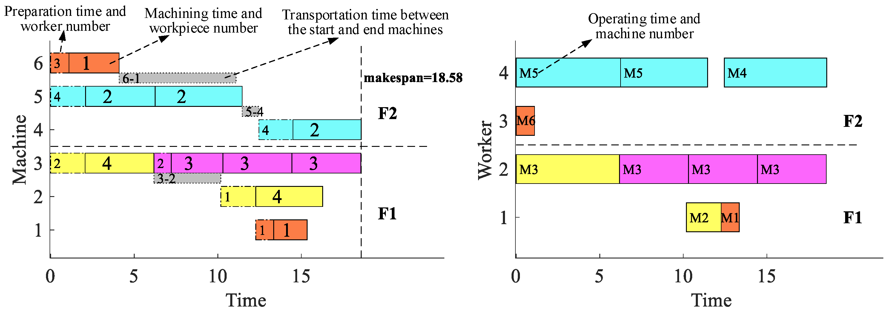
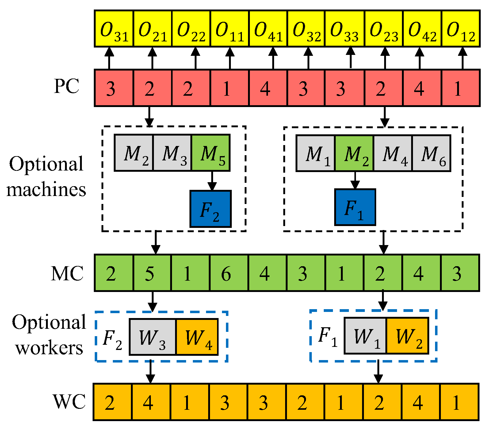
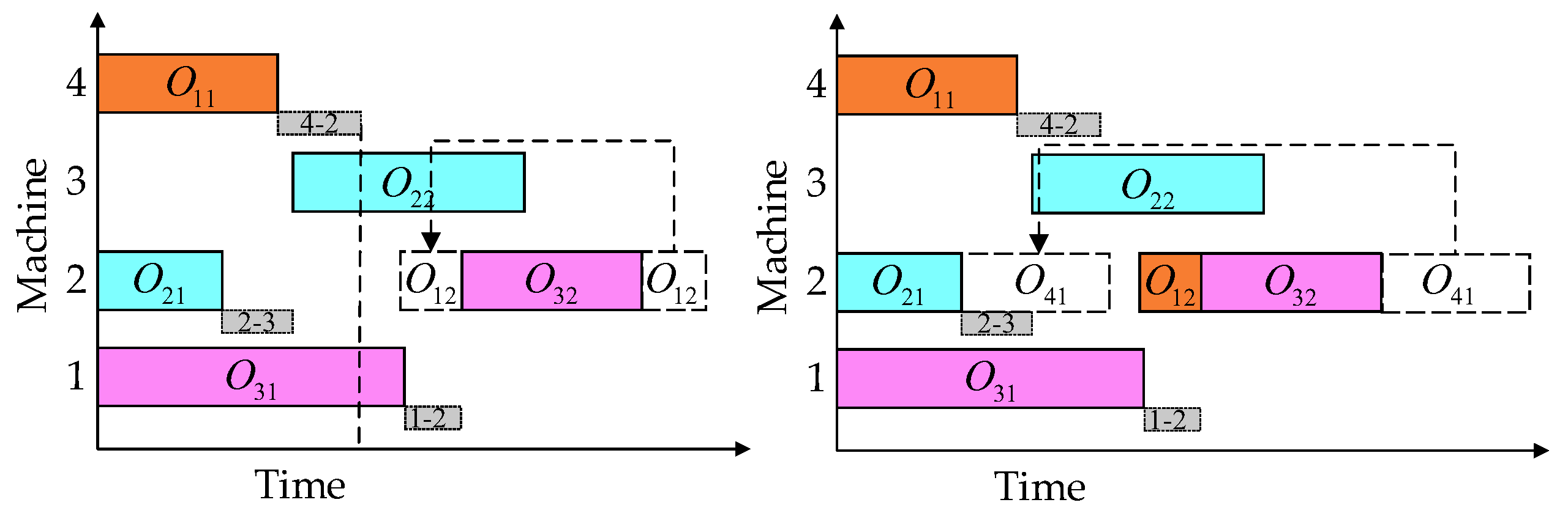
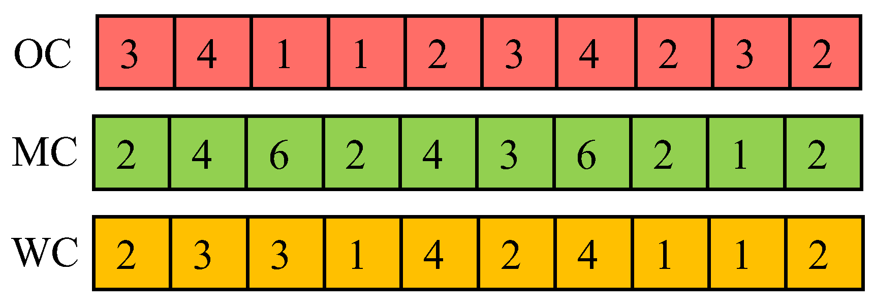
3.3. Coding and Decoding

According to the problem characteristics of DFJSPD, each mayfly individual represents a solution that contains multiple information of process, factory, machine, and worker. This paper adopts a three-layer coding method: process coding (OC), machine coding (MC), and worker coding (WC). The three vector elements are in one-to-one correspondence, and the factory selection is reflected by machine coding. Considering the data in Table 1 as an example, the coding is shown in Figure 2. The three-layer codes are read from left to right at the same time. Each number in OC represents the workpiece number of the $j$th occurrence in turn, and $j$ is the process number of the workpiece. The corresponding positions of MC and WC represent the machine that processes the process and the worker who operates the machine.

A feasible solution code can show only the resources allocation information, and the complete scheduling scheme needs to be obtained by decoding. The most commonly used decoding method is the insertion decoding, as shown in Figure 3. Each process is arranged in the earliest processing time of the available idle time window. This method can effectively reduce the waste of idle time, but the utilization of idle time window may not be high.

Therefore, this paper designs an active time window decoding algorithm considering transportation time for DFJSPD. The key is that when a process can be properly adjusted within the available idle time window, the start time is determined at the latest end time, and the larger idle time window is left as far as possible for subsequent processes, as shown in Figure 4. According to the process, transportation time, machine type, and flexible constraints of machine and worker in DFJSPD, as well as whether the preparation time and machining time of each process are affected, are judged and arranged in an appropriate idle time window. The steps of decoding are summarized by the pseudo code shown in Algorithm 2. The main steps are as follows:

Traverse three-layer codes to obtain a process, the selected machine and worker, and the start and stop time of the idle time window of machine and worker;

According to Equations (2)–(8), the actual processing time and the earliest start time of the process are calculated;

Traverse the available idle time window, compare the remaining idle time window after insertion and $ave{T}_k$ to determine the actual start time of the process. $ave{T}_k$ is the average processing time of all processes on the machine, as shown in (10):

$$ave{T}_k=\frac{{\displaystyle \sum _{h=1}^n{\displaystyle \sum _{g=1}^{n_i}(X_{hgk}T{l}_{hgk}+X_{hgk}{T}_{hgk}}})}{{\displaystyle \sum _{h=1}^n{\displaystyle \sum _{g=1}^{n_i}{X}_{hgk}}}}$$

(10)

Determine the actual end time of the process, update the idle time window, and decode the next process until all the processes are completed.

Algorithm 2. Pseudo code of the active time window decoding algorithm.

TO←Total processes for o = 1: TO $O_{ij}$ = OC(o), $M_k$ = MC(o), $W_s$ == WC(o)   $Mspan\left\{k\right\}$←the idle time windows of $M_k$   $Wspan\left\{s\right\}$←the idle time windows of $W_s$   //$STXspan$ and $ETXspan$ indicates the start and end time of the idle time window $X$   If $j$ == 1   $A_{ij}=C_{i(j-1)}+T{Y}_{lk}$; $YT=T{Y}_{lk}$   Else   $A_{ij}=0$; $YT=0$   End if   If $H_k$ == 1     im←total available idle time windows of $M_k$     $Mspan\left\{k\right\}(z)$←the $z$th available idle time window of $M_k$     $Wspan\left\{s\right\}(x)$←the $x$th available idle time window of $W_s$     For $z$ = 1:im     If $STMspan\left\{k\right\}(z)$ == $C_{i(j-1)}$     $WT=PT=0$; $MT=T_{ijk}$; $S_{ijks}=\max \{A_{ij},STMspan\{k\}(z)\}$     Else       $MWspan=Wspan\left\{s\right\}\cap [STMspan\{k\}(z),ETMspan\{k\}(z)-MT]$       $x$ = find ($Wspan\left\{s\right\}\supseteq MWspan$)       If $ETMWspan-STMWspan$>$WT$       $Lp=\min (ETWspan\{s\}(x),ETMspan\{k\}(z)-MT)$       Else       End if Else if End for $z$ If $Lp-PT-STMspan\left\{k\right\}(z)>=ave{T}_k$ $S_{ijks}=Lp-PT$ Else $S_{ijks}=\max \{A_{ij},STWMspan\}$ End if Else     $MWspan=Mspan\left\{k\right\}\cap Wspan\left\{s\right\}$     it←total $MWspan$     for $i$ = 1:it       $m$ = find ($Mspan\left\{k\right\}\supseteq MWspan(i)$)     If $STMspan\left\{k\right\}(m)$ == $C_{i(j-1)}$     $PT=0$; $MT=T_{ijk}/e_{ks}$; $WT=MT$;     Else     $PT=T{l}_{ijk}/e_{ks}$; $MT=T_{ijk}/e_{ks}$; $WT=PT+MT$     End if       If $A_{ij}>STMWspan(i)$&& $(ETMWspan(i)-STMWspan(i)-PT-MT)>=ave{T}_k$       $S_{ijks}=ETMWspan(i)-PT-MT$       break       Else       $S_{ijks}=\max \{A_{ij},STWMspan(i)\}$       break       End if End for $i$ End if $C_{ijks}=S_{ijks}+PT+MT$ Update $Mspan\left\{k\right\}$ and $Wspan\left\{s\right\}$ End for o

3.4. Mixed Initialization

Initializing the population is the premise of intelligent algorithm optimization; the initial population quality has an important influence on the convergence speed and optimization ability of the algorithm. When setting the initial solution, it is necessary to improve the quality of the solution according to the optimization objective. In addition, the diversity of the initial solution should be ensured to avoid the population falling into local optimum. In this paper, that initial position vector of mayfly is discrete mapped for OC, and a variety of initialization rules considering time (population ratio is 4:2:2:1:1) are designed for the corresponding MC and OC.

Heuristic rule based on completion time: Each process in OC is traversed successively to select the worker–machine combination that can minimize the completion time.

Global initialization rule: Each process of each workpiece is traversed successively, and the worker–machine combination for the shortest total cumulative processing time is selected for it.

Local initialization rule: Each process of each workpiece is traversed in turn to select the worker–machine combination for the shortest cumulative processing time of the workpiece.

Single initialization rule: Each process in OC is traversed successively to select the worker–machine combination that can minimize the processing time.

Random initialization rule: Each process in OC is traversed successively to select any worker–machine combination that can process the process.

3.5. Updating of Mayfly

The male mayfly in MA constantly adjusts its velocity and direction according to its historical optimal position $(pbest)$ and the optimal position in the population $(gbest)$ to move towards the optimal position. When the male mayfly is in the best position, the wedding dance mode is executed, and its velocity varies according to inertia weight and dance coefficient. The update formulas of the velocity and position of male mayfly are as follows:

$$m{v}_{ij}^{t+1}=\{\begin{array}{ll}g\ast m{v}_{ij}^t+a_1{e}^{-\beta r_p^2}\left(pbes{t}_{ij}-x_{ij}^t\right)+a_2{e}^{-\beta r_g^2}\left(gbes{t}_j-x_{ij}^t\right),& \mathrm{if}f(x_i)>f(gbest)\\ g\ast m{v}_{ij}^t+d\ast r,& \mathrm{if}f(x_i)\le f(gbest)\end{array}$$

(11)

$$x_{ij}^{t+1}=x_{ij}^t+m{v}_{ij}^{t+1}$$

(12)

where $m{v}_{ij}^t$ is the velocity of the male mayfly $i$ in dimension $j$ at time step $t$. $g$ is the inertia weight. $a_1$ and $a_2$ are positive attraction constants used to scale the contribution of the cognitive and social component respectively. $\beta$ is a fixed visibility coefficient. $d$ is the nuptial dance coefficient. $r$ is a random value in the range [–1,1]. $r_p$ is the Cartesian distance between $x_i^t$ and $pbes{t}_{ij}$, and $r_g$ is the Cartesian distance between $x_i^t$ and $gbes{t}_j$. In Equation (12), $x_{ij}^t$ is the position of the male mayfly $i$ in dimension $j$ at time step $t$.

In order to reproduce offspring, female mayflies are attracted by male mayflies. They adjust their velocity and direction to fly towards male mayflies and keep approaching. When a female mayfly is not attracted by a male mayfly, it flies randomly. The update formulas of the velocity and position of female mayfly are as follows:

$$f{v}_{ij}^{t+1}=\{\begin{array}{ll}g\ast f{v}_{ij}^t+a_2{e}^{-\beta r_{mf}^2}\left(x_{ij}^t-y_{ij}^t\right),& \mathrm{if}f(y_i)>f(x_i)\\ g\ast f{v}_{ij}^t+fl\ast r,& \mathrm{if}f(y_i)\le f(x_i)\end{array}$$

(13)

$$y_{ij}^{t+1}=y_{ij}^t+f{v}_{ij}^{t+1}$$

(14)

where $f{v}_{ij}^t$ is the velocity of the female mayfly $i$ in dimension $j$ at time step $t$. $fl$ is a randomly walk coefficient, and $r_{mf}$ is the Cartesian distance between male and female mayflies. In Equation (12), $y_{ij}^t$ is the position of the female mayfly $i$ in dimension $j$ at time step $t$.

In order to balance the global exploitation and local exploration in the early and late stages of the algorithm, the dynamic inertia weight is adopted [19], which linearly decreases with the number of iterations. After the mayfly position is updated, it is mapped to process code according to the discrete method in Section 3.2. The original worker–machine combination of each process is unchanged, and their positions are changed accordingly. After updating the position of mayfly corresponding to the process code in Figure 2, the three-layer codes after discrete mapping are as shown in Figure 5.

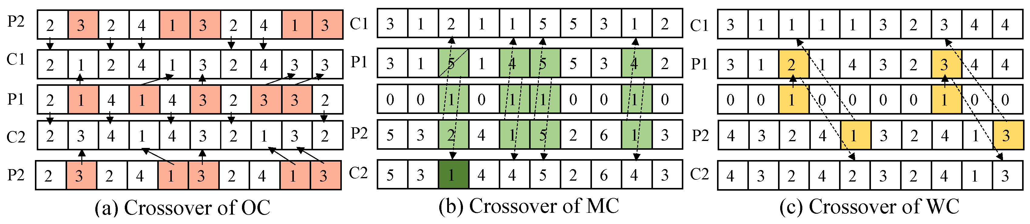
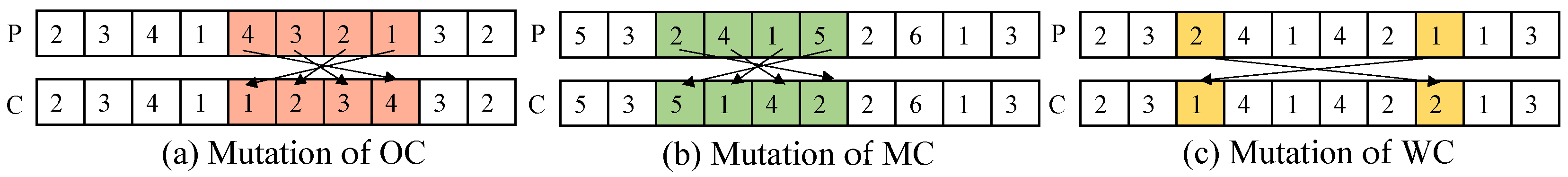
3.6. Crossover and Mutation Operators

The crossover operation of the original MA algorithm is based on the quality of the solution. A male mayfly breeds with the female mayfly at the same fitness level with it; however, the original crossover formula is applicable to the continuous optimization problem [25]. Therefore, in this paper, crossover and mutation operators are designed respectively for the characteristics of the three-layer codes.

(1) Crossover operator

(a) The IPOX crossover operator is adopted on OC. (b) An improved IMPX crossover operator [26] is adopted on MC. If the machine is unavailable after exchanging, a machine with the shortest processing time is selected from the set of alternative machines for the corresponding process. (c) Since it is assumed that workers cannot transfer across factories, a two-point crossover operator considering factory constraint is designed for WC. For the parent P1, two crossover points are selected and exchanged respectively with any two workers in the same factory in the parent P2. If the worker after the exchange is unavailable, a worker with the highest efficiency is selected in the optional workers set for the corresponding machine. Three crossover operators are shown in Figure 6, where P represents the parent and C represents the offspring.

(2) Mutation operator

(a) Reverse sequence mutation is adopted on OC. The genes reverse sequence exchange between two different mutation sites randomly selected, and MC and WC are adjusted accordingly to keep the original worker–machine combination of each process unchanged. (b) The mutation rules on MC are the same as OC, and if the machine after mutating is unavailable, the worker–machine combination is reselected in the optional machines and workers set. (c) Two points of mutation are adopted on WC, that is, randomly selecting two different workers in a factory to exchange positions. If the worker after the exchange is unavailable, a worker with the highest efficiency is selected in the optional workers set for the corresponding machine. The three mutation operators are shown in Figure 7.

4. Experiment and Analysis

4.1. Testing Instances and Parameter Setting

Since there are few previous studies on DFJSPD, there are no relevant benchmark instances for reference and test. This paper designed 20 DFJSPD instances of isomorphism and isomerism factories by extending 10 FJSP benchmarks of Brandimarte [27] that are widely applicable in the field of FJSP and used by a large number of researchers [9,28,29].

(1) Isomorphism factories instances (SMk01-SMk10)

The quantity and functional flexibility of machines and workers in isomorphism factories are the same. Set the workpieces processing time and the worker–machine information and copy these to construct factories F1 and F2 with the same processing environment.

(2) Isomerism factories instances (DMk01-DMk10)

There are differences in the number and function flexibility of machines and workers in isomerism factories. Split the machine information and the number of workers of factory F1 in isomorphism factories instances to construct factories F1 and F2, respectively; workers’ skills in each factory are completely flexible.

For any instance, the process preparation time is generated in $U[2,8]$, the worker efficiency is generated randomly in $U[0.8,1.2]$, the transportation time between machines in the same factory is generated in $U[1,5]$, and the transportation time between machines in different factories is generated in $U[6,10]$ [9]. A total of 30% of the machines are selected as CNC machines. The scale and machines information of each instance are shown in

Table 4. Descriptions of the DFJSPD instances.

Isomorphism Factories Instance	Scale	CNC Machines	Isomerism Factories Instance	Scale	CNC Machines
	$\mathit{n}\times \mathit{(}\mathit{m}\times \mathit{w}\mathit{)}\times \mathit{f}$			$\mathit{n}\times \mathit{(}\mathit{m}\times \mathit{w}\mathit{)}\times \mathit{f}$
SMk01	10 × (6 × 4) × 2	2,4,8,10	DMk01	10 × (3 × 2) × 2	2,4
SMk02	10 × (6 × 4) × 2	2,4,8,10	DMk02	10 × (3 × 2) × 2	2,4
SMk03	15 × (8 × 6) × 2	1,8,9,16	DMk03	15 × (4 × 3) × 2	1,8
SMk04	15 × (8 × 6) × 2	1,3,9,11	DMk04	15 × (4 × 3) × 2	1,3
SMk05	15 × (4 × 3) × 2	3,7	DMk05	15 × (2 × 2) × 2	3
SMk06	10 × (15 × 8) × 2	2,3,4,7,17,18,19,22	DMk06	10 × ((8 × 4) + (7 × 4))	2,3,4,7
SMk07	20 × (5 × 4) × 2	2,7	DMk07	20 × ((3 × 2) + (2 × 2))	2
SMk08	20 × (10 × 6) × 2	1,3,10,11,13,20	DMk08	20 × (5 × 3) × 2	1,3,10
SMk09	20 × (10 × 6) × 2	2,4,8,12,14,18	DMk09	20 × (5 × 3) × 2	2,4,8
SMk10	20 × (15 × 8) × 2	2,3,7,10,17,18,22,25	DMk10	20 × ((8 × 4) + (7 × 4))	2,3,7,10

. $n\times (m\times w)\times F$ represents $n$ workpieces processed in $F$ factories, and $m$ machines and $w$ workers are in each factory.

To verify the superior performance of IMA, it was compared with the results of traditional MA, GA, PSO, and FA algorithms. Traditional algorithms adopt three-layer encoding, random initialization, and insertion decoding methods. The parameter settings of the algorithms are shown in

Table 5. Parameters setting of algorithms.

Algorithm	Population Scale	Number of Iterations	Other Parameters
IMA	female: 50, male: 50	200	$\begin{array}{c}{a}_1=1,a_2=a_3=1.5,\beta =2,d=fl=1,\\ g_{\max }=1.5,g_{\min }=0.4\end{array}$
MA	female: 50, male: 50	200	$a_1=1,a_2=a_3=1.5,\beta =2,d=fl=1,g=0.8$
GA	100	200	crossover rate 0.8, mutation rate 0.05
PSO	100	200	inertia weight $\omega =0.8$, learning factor $c_1=c_2=2$
FA	100	200	attractiveness of firefly ${\beta }_0=1$, light absorption coefficient $\gamma =1$, random parameter $\alpha =0.3$

. All experiments are run on MATLAB R2020a.

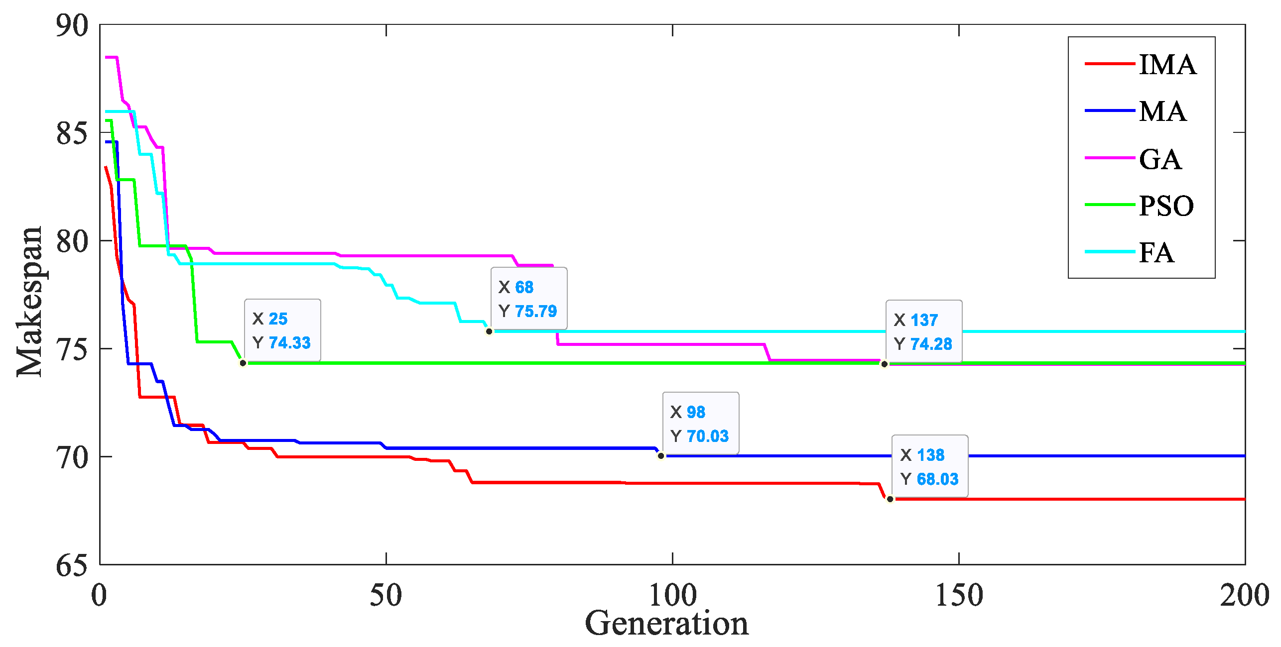
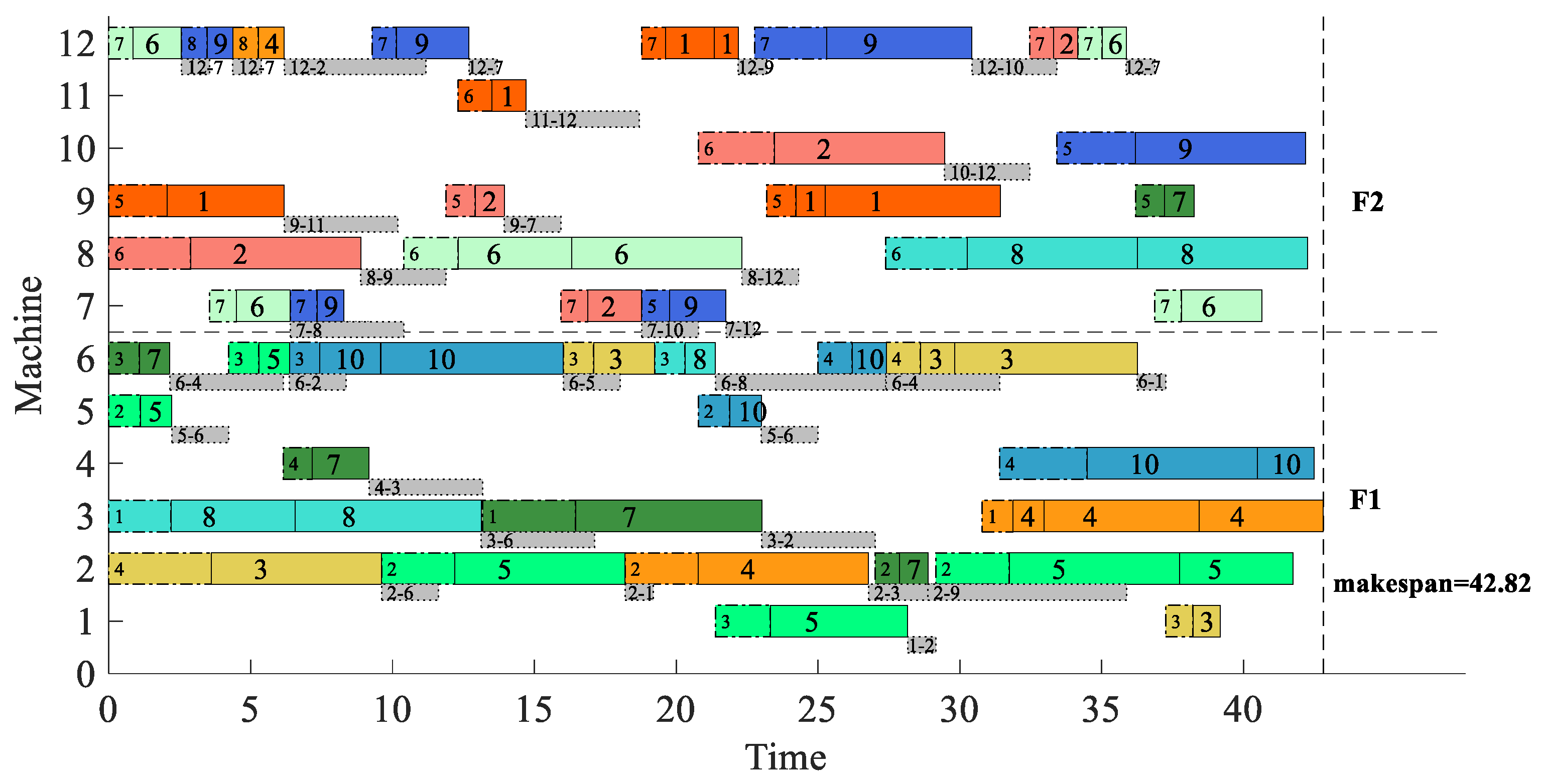
4.2. Results Analysis

In order to avoid random differences, each instance is solved 20 times by each algorithm, and the results of isomorphism and isomerism factories instances are shown in

Table 6. The results of isomorphism factories instances.

	IMA		MA		GA		PSO		FA
	${\mathit{C}}_{\mathbf{max}}^{\mathbf{min}}$	${\mathit{C}}_{\mathbf{max}}^{\mathit{a}\mathit{v}\mathit{e}}$	${\mathit{C}}_{\mathbf{max}}^{\mathbf{min}}$	${\mathit{C}}_{\mathbf{max}}^{\mathit{a}\mathit{v}\mathit{e}}$	${\mathit{C}}_{\mathbf{max}}^{\mathbf{min}}$	${\mathit{C}}_{\mathbf{max}}^{\mathit{a}\mathit{v}\mathit{e}}$	${\mathit{C}}_{\mathbf{max}}^{\mathbf{min}}$	${\mathit{C}}_{\mathbf{max}}^{\mathit{a}\mathit{v}\mathit{e}}$	${\mathit{C}}_{\mathbf{max}}^{\mathbf{min}}$	${\mathit{C}}_{\mathbf{max}}^{\mathit{a}\mathit{v}\mathit{e}}$
SMk01	42.82	43.86	45.21	46.26	46.83	47.66	46.49	47.38	47.22	48.04
SMk02	31.78	32.39	32.93	33.38	33.10	33.43	33.70	34.66	34.53	35.11
SMk03	154.28	156.06	155.38	157.77	155.86	156.89	164.85	165.28	163.59	165.03
SMk04	63.83	65.63	67.60	68.39	66.51	67.89	68.53	69.99	67.70	69.51
SMk05	142.02	145.27	147.78	149.69	149.21	156.52	148.93	154.08	150.30	158.20
SMk06	91.66	93.02	93.94	94.77	94.12	95.09	96.18	97.57	95.69	96.47
SMk07	122.00	124.35	126.06	128.36	126.30	128.19	128.67	131.26	127.30	130.64
SMk08	430.00	435.96	445.59	447.21	441.00	447.72	446.53	453.16	447.31	451.48
SMk09	319.41	321.98	329.40	332.58	330.24	334.33	349.96	351.68	342.18	346.66
SMk10	237.13	240.55	245.76	256.69	248.64	259.62	252.78	256.63	260.37	262.41

and

Table 7. The results of isomerism factories instances.

	IMA		MA		GA		PSO		FA
	${\mathit{C}}_{\mathbf{max}}^{\mathbf{min}}$	${\mathit{C}}_{\mathbf{max}}^{\mathit{a}\mathit{v}\mathit{e}}$	${\mathit{C}}_{\mathbf{max}}^{\mathbf{min}}$	${\mathit{C}}_{\mathbf{max}}^{\mathit{a}\mathit{v}\mathit{e}}$	${\mathit{C}}_{\mathbf{max}}^{\mathbf{min}}$	${\mathit{C}}_{\mathbf{max}}^{\mathit{a}\mathit{v}\mathit{e}}$	${\mathit{C}}_{\mathbf{max}}^{\mathbf{min}}$	${\mathit{C}}_{\mathbf{max}}^{\mathit{a}\mathit{v}\mathit{e}}$	${\mathit{C}}_{\mathbf{max}}^{\mathbf{min}}$	${\mathit{C}}_{\mathbf{max}}^{\mathit{a}\mathit{v}\mathit{e}}$
DMk01	68.03	69.97	70.03	73.27	74.28	76.63	74.33	76.08	75.79	77.00
DMk02	45.56	47.38	46.03	47.99	46.54	48.63	48.74	50.60	48.39	50.70
DMk03	235.26	257.21	268.34	284.60	263.26	279.46	266.92	287.95	276.92	286.13
DMk04	104.51	111.52	114.19	117.74	112.84	118.54	118.45	122.00	116.93	122.60
DMk05	234.53	243.02	256.25	270.02	256.93	268.72	258.51	271.35	260.77	272.13
DMk06	133.89	142.71	153.49	158.90	150.54	159.85	153.72	161.22	157.08	160.73
DMk07	213.13	225.70	228.69	238.58	232.32	239.04	249.30	253.57	249.30	252.71
DMk08	735.70	765.51	788.57	811.98	770.23	805.96	801.65	836.58	781.34	844.57
DMk09	529.02	547.75	569.38	585.13	550.38	572.43	556.30	585.96	571.10	591.50
DMk10	428.64	447.54	458.24	463.94	446.04	469.25	468.68	480.76	466.86	479.06

. $C_{\max }^{\min }$ and $C_{\max }^{ave}$ are the optimal and mean value, respectively, of 20 results of an algorithm.

Table 6 and Table 7 show that due to the randomness of population initialization and evolution process, there are differences among the results of each example. Overall, the optimal value and mean value of IMA are less than other algorithms. The larger the scale of the example, the more obvious the difference. This shows that the active time window decoding can better coordinate resources and reduce idle time, especially when solving large-scale problems.

To significantly compare algorithms differences, two evaluation indicators are designed according to the literature [29]: the minimum value of relative percentage deviation (MRPD) and the average value of relative percentage deviation (ARPD). The calculation formulas are as follows:

$$MRPD=\frac{C_{\max }^{\min }-C_{\max }^{low}}{C_{\max }^{low}}\times 100$$

(15)

$$ARPD=\frac{1}{s}{\displaystyle \sum _{i=1}^s\left(\frac{C_{\max }^i-C_{\max }^{low}}{C_{\max }^{low}}\times 100\right)}$$

(16)

In Equations (15)–(16), for any instance, $C_{\max }^i$ is the $i$th result of an algorithm solving it, $C_{\max }^{low}$ is the optimal value of all the results of all the algorithms, $s$ is the number of iterations of solving. The smaller the MRPD, the better the accuracy of the algorithm convergence; the smaller the MRPD, the better the stability of the algorithm. The values of MRPD and ARPD are shown in

Table 8. Evaluation results of isomorphism factories instances.

Instance	${\mathit{C}}_{\mathbf{max}}^{\mathit{l}\mathit{o}\mathit{w}}$	IMA		MA		GA		PSO		FA
		MRPD	ARPD	MRPD	ARPD	MRPD	ARPD	MRPD	ARPD	MRPD	ARPD
SMk01	42.82	0	2.44	5.58	8.04	9.36	11.31	8.57	10.65	10.28	12.19
SMk02	31.78	0	1.91	3.62	5.04	4.15	5.20	6.04	9.06	8.65	10.47
SMk03	154.28	0	1.16	0.71	2.26	1.02	1.69	6.85	7.13	6.03	6.97
SMk04	63.83	0	2.77	5.86	7.10	4.15	6.31	7.31	9.59	6.01	8.84
SMk05	142.02	0	2.29	4.06	5.40	5.06	10.21	4.87	8.49	5.83	11.39
SMk06	91.66	0	1.49	2.49	3.39	2.68	3.74	4.93	6.45	4.39	5.24
SMk07	122.00	0	1.93	3.33	5.21	3.52	5.07	5.47	7.59	4.34	7.09
SMk08	430.00	0	1.39	3.63	4.00	2.56	4.12	3.84	5.39	4.03	5.00
SMk09	319.41	0	0.80	3.13	4.12	3.39	4.67	9.56	10.10	7.13	8.53
SMk10	237.13	0	1.44	3.64	8.25	4.85	9.48	6.60	8.22	9.80	10.66

and

Table 9. Evaluation results of isomerism factories instances.

Instance	${\mathit{C}}_{\mathbf{max}}^{\mathit{l}\mathit{o}\mathit{w}}$	IMA		MA		GA		PSO		FA
		MRPD	ARPD	MRPD	ARPD	MRPD	ARPD	MRPD	ARPD	MRPD	ARPD
DMk01	68.03	0	2.85	2.94	7.70	9.19	12.64	9.26	11.84	11.41	13.18
DMk02	45.56	0	4.00	1.03	5.34	2.15	6.73	6.98	11.07	6.21	11.28
DMk03	235.26	0	9.33	14.06	20.97	11.90	18.79	13.46	22.39	17.71	21.62
DMk04	104.51	0	6.71	9.26	12.66	7.97	13.43	13.34	16.73	11.88	17.31
DMk05	234.53	0	3.62	9.26	15.13	11.19	16.03	10.22	15..70	9.55	14.58
DMk06	133.89	0	6.59	15.39	18.83	12.44	19.39	14.81	20.41	17.32	20.04
DMk07	213.13	0	5.90	7.30	11.94	9.00	12.16	16.97	18.98	16.97	18.57
DMk08	735.70	0	4.05	7.19	10.37	4.69	9.55	8.96	13.71	6.20	14.80
DMk09	529.02	0	3.54	7.63	10.61	4.04	8.20	5.16	10.76	7.95	11.81
DMk10	428.64	0	4.41	6.91	8.24	4.06	9.47	9.38	12.16	8.92	11.76

.

From Table 8 and Table 9, it can be seen that all the MRPD values of IMA for 20 DFJSPD instances are 0, that is, the optimal results of IMA are the best in all algorithms which indicates that IMA converges more accurately than others. In most instances, the differences of MRPD values between MA and GA are small, and the probability of obtaining the suboptimal solution is greater than PSO and FA; this indicates that the crossover and mutation operations of MA and GA can expand the search range and improve the probability of obtaining the better solution, while the operation of updating the position according to the better solution of PSO and FA has low solution accuracy and can easily fall into local optimum. Comparing the values of ARPD, the average performance of IMA is better than MA, GA, PSO, and FA, which shows that IMA hybrid initialization strategy and improved crossover and mutation operators generally improve the solution quality and stability of the algorithm.

Average CPU time of all instances are listed in

Table 10. Average CPU time.

Instance	Average CPU Time/s					Instance	Average CPU Time/s
	IMA	MA	GA	PSO	FA		IMA	MA	GA	PSO	FA
SMk01	10.21	9.72	10.21	10.06	10.38	DMk01	13.20	12.93	13.05	13.16	13.38
SMk02	11.67	10.64	11.30	10.81	11.94	DMk02	13.40	13.02	13.27	13.04	13.48
SMk03	39.31	38.51	39.46	38.67	39.84	DMk03	44.02	43.48	43.87	43.67	44.05
SMk04	12.14	11.60	12.67	11.97	12.25	DMk04	17.15	16.64	17.14	16.90	17.19
SMk05	41.52	39.57	41.54	40.49	41.81	DMk05	46.23	45.32	46.12	45.63	46.30
SMk06	35.37	31.60	34.08	32.19	34.81	DMk06	40.80	37.67	38.14	37.87	40.42
SMk07	31.72	27.54	29.61	27.93	30.64	DMk07	38.48	34.14	36.80	34.67	37.39
SMk08	80.80	76.43	77.64	76.85	80.30	DMk08	106.91	102.45	103.61	102.64	106.67
SMk09	79.31	74.15	75.34	74.36	78.48	DMk09	99.87	96.32	97.60	96.93	98.18
SMk10	68.10	64.16	66.49	64.89	67.07	DMk10	87.75	83.40	85.69	83.36	86.55

.

It can be seen from isomorphism instances in Table 10 that the IMA costs 6.83% more CPU time than MA, 2.96% more than GA, 5.65% more than PSO, and 0.65% more than FA, on average. It can be seen from isomerism instances in Table 10 that the IMA costs 4.62% more CPU time than MA, 2.53% more than GA, 4.09% more than PSO, and 0.83% more than FA, on average. In addition, as the scale of the problem increases, IMA costs more CPU time than other algorithms. This indicates that the discrete mapping, crossover, and mutation strategies of IMA can slightly reduce the computational efficiency, especially for large-scale problems.

The convergence performance of the algorithm is analyzed by considering example DMk01. It can be seen from Figure 8 that the hybrid initialization strategy of IMA improves the quality of the initial population. The five algorithms can converge to their respective optimal solutions, but the convergence speed of GA and FA is slow and the solution accuracy is low, converging to 74.28 and 75.79, respectively. PSO has the fast convergence speed, but it is subject to premature converging to 74.33. The convergence speeds of IMA and MA are fast in the early stage, and the completion time converges to approximately 70 in the 30th generation. The wedding dance and random flight operations in the late iteration make the algorithm jump out of local optimum, but the accuracy of the crossover and mutation methods of MA is not high, converging to 70.03. The multiple crossover and mutation operators of IMA can expand the search range, and found the optimal solution at 68.03. Overall, the optimization ability and speed of IMA are better than other four algorithms.

From the Gantt charts of the optimal solutions of SMk01 and DMk01 in Figure 9, Figure 10, Figure 11 and Figure 12, it can be seen that the scheduling schemes of the same number of workpieces in distributed factories with different structures are different, and the final completion time is also different. Workpieces are circulated among multiple open structure factories, and the processing resources of each factory can be fully utilized in time. The workpieces are transferred among multiple open structure factories, which can make full use of the processing resources of each factory timely. The more comprehensive the resources, the higher the processing efficiency. This paper can provide a more clear and accurate scheduling scheme for distributed factories collaborative intelligent manufacturing with different structures.

5. Conclusions

In the actual distributed flexible job shop production process, the worker–machine dual resource constraints and the transportation time of workpiece flowing among machines seriously affect the scheduling plan. In order to construct a scheduling model that is more in line with the actual processing situation, this paper establishes the DFJSPD model with the optimization objective of the minimum of maximum completion time. For the multiple constraints of the discrete DFJSPD problem, the mayfly algorithm is improved by using the discrete mapping method of continuous variables, three-layer coding, decoding algorithm of an active time window, hybrid initialization strategy, and the crossover and mutation operator of three-layer codes to improve the global exploitation and local exploration performance of MA. Finally, the basic instances are expanded to design the instances of isomorphism and isomerism factories. The simulation experiments are carried out and compared with various algorithms. The results show that IMA is superior to other algorithms in terms of solution quality and stability without a sharp decrease in the solution efficiency. The model and algorithm in this paper can help enterprises realize distributed collaborative intelligent manufacturing.

However, the above research is still insufficient and needs to be further optimized. In the practical production environment, transport resources are not at one’s unlimited disposal, and this paper had a lack of consideration of transport resources constraints. In addition, the IMA has the defect of low computational efficiency while solving large-scale DFJSPD problems, which will affect production efficiency. Therefore, in the future, this paper will study DFJSP scheduling methods under more resource constraints and explore intelligent scheduling algorithms with better performance and efficiency.

References

1. Viana, M.S.; Contreras, R.C.; Morandin Junior, O. A New Frequency Analysis Operator for Population Improvement in Genetic Algorithms to Solve the Job Shop Scheduling Problem. Sensors 2022, 22, 4561. [Google Scholar] [CrossRef] [PubMed]
2. Wang, K. Migration strategy of cloud collaborative computing for delay-sensitive industrial IoT applications in the context of intelligent manufacturing. Comput. Commun. 2020, 150, 413–420. [Google Scholar] [CrossRef]
3. Zhou, L.; Jiang, Z.; Geng, N.; Niu, Y.; Cui, F.; Liu, K.; Qi, N. Production and operations management for intelligent manufacturing: A systematic literature review. Int. J. Prod. Res. 2022, 60, 808–846. [Google Scholar] [CrossRef]
4. Jiang, Z.; Yuan, S.; Ma, J.; Wang, Q. The evolution of production scheduling from Industry 3.0 through Industry 4.0. Int. J. Prod. Res. 2021, 60, 3534–3554. [Google Scholar] [CrossRef]
5. Huang, J.; Chang, Q.; Arinez, J. Distributed Production Scheduling for Multi-Product Flexible Production Lines. In Proceedings of the 16th International Conference on Automation Science and Engineering (CASE), Hong Kong, 20–21 August 2020; pp. 1473–1478. [Google Scholar]
6. Shao, W.; Shao, Z.; Pi, D. Modeling and multi-neighborhood iterated greedy algorithm for distributed hybrid flow shop scheduling problem. Knowl.-Based Syst. 2020, 194, 105527. [Google Scholar] [CrossRef]
7. De Giovanni, L.; Pezzella, F. An improved genetic algorithm for the distributed and flexible job-shop scheduling problem. Eur. J. Oper. Res. 2010, 200, 395–408. [Google Scholar] [CrossRef]
8. Ziaee, M. A heuristic algorithm for the distributed and flexible job-shop scheduling problem. J. Supercomput. 2014, 67, 69–83. [Google Scholar] [CrossRef]
9. Sang, Y.; Tan, J. Intelligent factory many-objective distributed flexible job shop collaborative scheduling method. Comput. Ind. Eng. 2022, 164, 107884. [Google Scholar] [CrossRef]
10. Xu, W.; Hu, Y.; Luo, W.; Wang, L.; Wu, R. A multi-objective scheduling method for distributed and flexible job shop based on hybrid genetic algorithm and tabu search considering operation outsourcing and carbon emission. Comput. Ind. Eng. 2021, 157, 107318. [Google Scholar] [CrossRef]
11. Meng, L.; Zhang, C.; Ren, Y.; Zhang, B.; Lv, C. Mixed-integer linear programming and constraint programming formulations for solving distributed flexible job shop scheduling problem. Comput. Ind. Eng. 2020, 142, 106347. [Google Scholar] [CrossRef]
12. Luo, Q.; Deng, Q.; Gong, G.; Zhang, L.; Han, W.; Li, K. An efficient memetic algorithm for distributed flexible job shop scheduling problem with transfers. Expert Syst. Appl. 2020, 160, 113721. [Google Scholar] [CrossRef]
13. Gong, G.; Chiong, R.; Deng, Q.; Luo, Q. A memetic algorithm for multi-objective distributed production scheduling: Minimizing the makespan and total energy consumption. J. Intell. Manuf. 2020, 31, 1443–1466. [Google Scholar] [CrossRef]
14. Du, Y.; Li, J.-Q.; Luo, C.; Meng, L.-L. A hybrid estimation of distribution algorithm for distributed flexible job shop scheduling with crane transportations. Swarm Evol. Comput. 2021, 62, 100861. [Google Scholar] [CrossRef]
15. Meng, L.; Zhang, C.; Zhang, B.; Ren, Y. Mathematical Modeling and Optimization of Energy-conscious Flexible Job Shop Scheduling Problem with Worker Flexibility. IEEE Access 2019, 7, 68043–68059. [Google Scholar] [CrossRef]
16. Obimuyiwa, D. Solving Flexible Job Shop Scheduling Problem in the Presence of Limited Number of Skilled Cross-Trained Setup Operators. Ph.D. Thesis, University of Guelph, Guelph, Canada, 2020. [Google Scholar]
17. Gong, G.; Chiong, R.; Deng, Q.; Gong, X. A hybrid artificial bee colony algorithm for flexible job shop scheduling with worker flexibility. Int. J. Prod. Res. 2020, 58, 4406–4420. [Google Scholar] [CrossRef]
18. Zhang, S.; Du, H.; Borucki, S.; Jin, S.; Hou, T.; Li, Z. Dual resource constrained flexible job shop scheduling based on improved quantum genetic algorithm. Machines 2021, 9, 108. [Google Scholar] [CrossRef]
19. Zervoudakis, K.; Tsafarak, S. A mayfly optimization algorithm. Comput. Ind. Eng. 2020, 145, 106559. [Google Scholar] [CrossRef]
20. Zarrouk, R.; Bennour, I.E.; Jemai, A. A two-level particle swarm optimization algorithm for the flexible job shop scheduling problem. Swarm Intell. 2019, 13, 145–168. [Google Scholar] [CrossRef]
21. Nayak, S.; Sood, A.K.; Pandey, A. Integrated Approach for Flexible Job Shop Scheduling Using Multi-objective Genetic Algorithm. In Advances in Mechanical and Materials Technology; Springer: Singapore, 2022; pp. 387–395. [Google Scholar]
22. Miller-Todd, J.; Steinhöfel, K.; Veenstra, P. Firefly-inspired algorithm for job shop scheduling. In Adventures between Lower Bounds and Higher Altitudes; Springer: Cham, Switzerland, 2018; pp. 423–433. [Google Scholar]
23. Gupta, J.; Nijhawan, P.; Ganguli, S. Parameter estimation of fuel cell using chaotic Mayflies optimization algorithm. Adv. Theory Simul. 2021, 4, 2100183. [Google Scholar] [CrossRef]
24. Mo, S.; Ye, Q.; Jiang, K.; Mo, X.; Shen, G. An improved MPPT method for photovoltaic systems based on mayfly optimization algorithm. Energy Rep. 2022, 8, 141–150. [Google Scholar] [CrossRef]
25. Xie, X.; Zheng, J.; Feng, M.; He, S.; Lin, Z. Multi-Objective Mayfly Optimization Algorithm Based on Dimensional Swap Variation for RFID Network Planning. IEEE Sens. J. 2022, 22, 7311–7323. [Google Scholar] [CrossRef]
26. Wu, R.; Li, Y.; Guo, S.; Xu, W. Solving the dual-resource constrained flexible job shop scheduling problem with learning effect by a hybrid genetic algorithm. Adv. Mech. Eng. 2018, 10, 1687814018804096. [Google Scholar] [CrossRef]
27. Brandimarte, P. Routing and scheduling in a flexible job shop by tabu search. Ann. Oper. Res. 1993, 41, 157–183. [Google Scholar] [CrossRef]
28. Lei, D.; Guo, X. Variable neighbourhood search for dual-resource constrained flexible job shop scheduling. Int. J. Prod. Res. 2014, 52, 2519–2529. [Google Scholar] [CrossRef]
29. Zheng, X.L.; Wang, L. A knowledge-guided fruit fly optimization algorithm for dual resource constrained flexible job-shop scheduling problem. Int. J. Prod. Res. 2016, 54, 5554–5566. [Google Scholar] [CrossRef]
Figure 1. Schematic diagram of DFJSPD scheduling.
Sustainability 14 12120 g001
Figure 2. Schematic diagram of coding.
Sustainability 14 12120 g002
Figure 3. Insertion decoding.
Sustainability 14 12120 g003
Figure 4. Active time window decoding.
Sustainability 14 12120 g004
Figure 5. The codes after updating of mayfly.
Sustainability 14 12120 g005
Figure 6. Crossover operators.
Sustainability 14 12120 g006
Figure 7. Mutation operators.
Sustainability 14 12120 g007
Figure 8. Algorithms iteration process diagram of DMk01.
Sustainability 14 12120 g008
Figure 9. The Machine Gantt chart of SMk01 with Optimal solution.
Sustainability 14 12120 g009
Figure 10. The Worker Gantt chart of SMk01 with Optimal solution.
Sustainability 14 12120 g010
Figure 11. The Machine Gantt chart of DMk01 with Optimal solution.
Sustainability 14 12120 g011
Figure 12. The Worker Gantt chart of DMk01 with Optimal solution.
Sustainability 14 12120 g012