Relationships between Organic Matter and Bulk Density in Amazonian Peatland Soils

Abstract

The carbon pool of Amazonian peatlands is immense and mediates critical ecological functions. As peatlands are dynamic, similar to other wetland systems, modeling of the relationship between organic matter and dry bulk density allows the estimation of the accumulation and/or decomposition of peats. We tested several models: the generalized linear mixed logarithmic, to test depth, and the non-linear logarithmic and power-law models. There is a negative power-law relationship between organic percentage and dry bulk density using peat samples collected in Amazonian peatlands (n = 80). This model is supported by the coefficient of determination (R²) estimates garnered from model fitting, while Akaike Information Criterion (AIC) values further support parsimonious models. We also ran trials of the ideal mixing model with two parameters: k1 representing organic density and k2 representing mineral. The mixture of organic and inorganic components generally falls in accordance with the theory that decreasing k1 trends with increasing k2, although k2 values for these peat samples are negative. The organic k1 coefficient allows us to identify two sites out of the nine investigated, which can be prioritized for their carbon dynamics. The presence of high-density samples, which were not related to depth, indicates clay intrusion in these peatlands. We hope the modeling can explain processes significant to these globally important carbon-rich ecosystems.

1. Introduction

Organic matter is a means of expressing carbon content in soils. Organic matter measurements are generally destructive and rely on the physical decomposition of organic matter at temperatures above 500 °C. Organic matter can then be expressed as a percentage of mass loss on ignition (LOI). This analysis has become routine in the study of peatlands [1,2,3,4]. This is intuitive, as the soil carbon pool of peatlands is immense [5,6,7].

It is well known that dry bulk density (DBD), one soil characteristic generated by LOI protocols, serves as an accurate predictor of carbon density in peat soil. This tendency has been proposed as a more rapid and efficient means of estimating large portions of carbon budgets [2,8]. Very little instrumentation and equipment are needed to derive DBD values from peat, but organic matter is more easily measured than total carbon (TC) using elemental analysis. The widespread use of TC elemental analysis in soils plays a role in carbon stock estimation [8,9], but incurs costs that are beyond the reach of many research projects, especially in the tropics.

In this process the exact significance of OM can be overlooked. Loss on ignition measures much larger volumes of peat than TC, so it can present more accurate assessment. In the case of peatlands, it is advisable to use OM as an explanatory variable for DBD, being the most readily ascertainable data. A multitude of studies have observed a nonlinear relationship between OM and DBD [10,11,12]. These studies often include peaty samples or highly organic soils, but usually take note of the relationship over a wider variety of soils down to very poor organic soils such as clay or rocky soils. This permits nonlinear modeling of soil data, which predicts soil characteristics over wider scales [13,14,15]. Few studies apply more than natural logarithmic models, while a variety of models can encompass the variation seen in patterns, e.g., power-law or negative exponential. Such models portend to have greater explanatory power then simple linear models, as diverse influences of geology, hydrology, or ecosystems can be involved [16,17,18,19]. The depths of the sampled soil types, though, often do not vary past thresholds less than 50 cm. This was the case in the noteworthy example in the Amazonian peatlands, where only ten samples exceeding 30 cm depth were measured [20]. The position of these samples seems to indicate that depth influences OM and DBD, but the arbitrary limit to depth constrains interpretation.

The presence of minerals in peat may relate to the site’s history with regard to mineral intrusion. In the Amazon, peatlands take part in a hydrologic cycle marked by persistent flood pulses, driving channel migrations, which can affect peatlands in a variety of acute or attenuated ways [21,22,23,24,25]. The introduction of surface water sources, carrying mineral components to peatlands, may be tied to such hydrologic drivers that play out over the millennial time scales involved in peatland formation [26,27,28,29,30,31,32,33]. In the most acute cases, peat burial may be a consequence [34,35,36]. In several Amazonian peatlands, buried peat layers have been documented [22,37]. These layers are separated by regions of clayey peat. This mineral presence could be interpreted as a sign of minerotrophy. While surface waterborne inputs vary over time, their mineral composition could be derived from the Varzea “whitewater” flood pulse [23,38].

Specific approaches to peatland sampling avoid taking clayey samples, assuming that they will not represent functional aspects of the ecosystems. The lack of clay-heavy samples in studies originating from Indonesian and central African sites may explain these biases [9,39]. The overall depth is another possible explanation, as some of the buried clay layers in Lähteenoja et al. [22] reside at depths greater than one–two meters, depths which in some studies are ignored. Shallower samples could help to elucidate processes more recent and significant to the current state of the ecosystem, potentially being in a steady state. Morris et al. [40] approached the steady-state of wetlands with variable surfaces by describing the behavior of OM in relation to DBD in the soils of North American coastal wetlands. Using nonlinear modeling, they found that an ideal mixing model best explained the relationship, and that based on principles of soil packing and volume, this model contains information about the wetlands’ organic and inorganic contributions to accretion or explicit rise in surface height. Such accretion is difficult to assess in tropical peatlands, although some of the coastal wetlands included in Morris et al. [40] were considered as peat above a 40% threshold of organic matter. This is markedly lower than that of Dargie et al. [39], who used a 65% OM threshold for tropical peatlands.

Complicated site histories in the Amazon [24,25,31] may imply that models take into account more factors driving peatland formation. While a given mineral component does not inherently support a particular source or process in the peatland, any means to increase understanding of ecosystemic processes relevant to peatlands will have further bearing upon the global importance of their carbon storage and potential sequestration [27,41]. Given the successes demonstrated in applying a wider variety of mathematical models to such routine descriptions of soil type, careful documentation of Amazonian peatland soil properties could enter into analyses indicative of processes significant to peat accumulation or burial. The strong 0.94 coefficient of determination for the logarithmic relationship found by Bhomia et al. [20] warrants further investigation into the phenomenon.

Objectives of this study:

• To find an adequate model for OM in relation to DBD in a sample of Amazonian peatlands;
• To test the significance of depth as a co-factor;
• Check for possible hydrological or landscape level effects in the site data;
• Assess the ideal mixing model.

2. Materials & Methods

Ucayali, Peru is a densely forested region in which annual rainfall is close to 2000 mm [42]. Extensive lowland zones are contained by near-Andean zones with high relief [43]. While coverage of acidic and poor entisols and inceptisols is high [44], further degradation due to extreme hydrologic conditions is expected [45,46,47], along with the occurrence of a variety of wetlands [48]. These pan-Amazonian trends likely apply to Ucayali, but only one study has addressed peatlands [49]. Junk et al. [50] identify Ucayali as under the influence of the Varzea flood pulse. (Figure 1) We were unable to undertake any geographic analyses for the purposes of this study.

2.1. Soil Sampling Process

Two hundred and thirty-two ten cm peat samples taken with a Russian corer [51] were acquired in Ucayali, Peru in 2016 and 2017. These samples come from a range of depths as each sample point involved the extraction of complete cores to refusal of the 5 cm Russian peat sampler (Aquatic Research Instruments, Hope, ID, USA). Sites 1–13 are independent repetitions of transects that repeat the sampling at different locations within the peatland. We determined the dry bulk density for all samples, while a subset of 80 was selected for full loss on ignition analysis, also following Chambers et al. [3]. In addition to low OM and/or high DBD, the clayey status of the samples could be observed in the field visually and by field texture test, aided by further reference to the photos taken of each core sample.

2.2. Quantitative

We carried out the Shapiro–Wilk normality test for the relevant datasets and residuals in R core [52] before proceeding to model fitting. We tested several models:

Logarithmic model:

DBD = x × ln (OM) + y

(1)

Logarithmic model with depth:

DBD = x × ln (OM) + y × depth + z

(2)

Power-law:

DBD = x OM^y

(3)

Power-law with intercept:

DBD = x OM^y + z

(4)

Ideal mixing model:

DBD = 1/ [OM/k1 + (1 − OM)/k2]

(5)

General linear models and Akaike Information Criterion (AIC) were calculated using the core statistics package. The generalized linear mixed model approach utilized the lme4 package [53]. Nonlinear model fitting was carried out in the minpack.lm package [54] using the Levenberg–Marquardt least-squares analysis. We treated residual sum-of-squares (RSS) as the coefficient of determination after:

$$R^2=1-RSS/ {\displaystyle \sum }{\left(DBD-\overline{DBD}\right)}^2$$

(6)

The McFadden’s pseudo-R² methodology applies to all non-linear models tested. Further assessment of models utilized the mean error (ME) and root mean square error (RMSE).

$$ME=\frac{1}{n}{{\displaystyle \sum }}_{i=1}^n\widehat{DB{D}_i}-DD{B}_i$$

(7)

$$RMSE=\sqrt{\frac{1}{n}}{{\displaystyle \sum }}_{i=1}^n{(\widehat{DB{D}_i}-DB{D}_i)}^2$$

(8)

$\widehat{DBD}$ is the predicted dry bulk density, and n is sample size.

To address significance in cofactors, the following correction equation was applied:

Depth(cm/Q) = D_samp × (Q/D_core)

(9)

where D_samp is sample depth, D_core is total depth of the core containing the sample, and Q is the third quartile value of all depth measurements taken.

3. Results

Loss on ignition analysis shows a range of values from 23 to 70% of organic matter (OM). The resulting data are normally distributed (W = 0.975, p = 0.1197), with a mean of 43.8%. With 42.1% median value, the majority of the samples (50 of 80) are above a 40% threshold of OM, while only four samples exceed 65%. In all but one site, these above −40% threshold samples come from at least half of the cores collected (

Table 1. Site descriptions: threshold columns show the number of samples that exceed the threshold, while the number of cores with samples exceeding the threshold is tallied in the next column. Sites included in the interval rows are varied, so min./max./thresholds are not applicable (n/a).

Site Number	Number of Points in Transect	Sample Size	Above 65% Thres- Hold	Above 40% Thres- Hold	Number of Cores over 40%	Average OM	Min. OM	Max. OM	Average DBD(g cm−3)	Average Depth (cm)	Min Depth	Max Depth
1	5	n = 8	0	2	2	34.8%	23.8%	54.9%	0.123	136	50	210
2	7	n = 8	0	4	4	37.3%	23.8%	57.5%	0.191	150	10	345
3	6	n = 14	1	11	5	46.4%	33.0%	68.5%	0.116	312	145	528
4	6	n = 10	0	6	4	45.9%	33.6%	61.8%	0.130	148	10	375
5	2	n = 9	0	6	2	42.5%	33.6%	52.3%	0.128	503	480	525
8	4	n = 4	1	2	2	45.9%	26.8%	67.0%	0.100	112	60	190
9	3	n = 4	0	3	2	51.0%	39.8%	61.5%	0.084	100	0	215
10	7	n = 15	0	11	7	44.8%	27.4%	63.8%	0.106	259	190	380
13	4	n = 8	2	5	4	47.1%	32.5%	70.7%	0.134	92	20	220
All sites	44	n = 80	4	50	32	43.8%	23.8%	70.7%	0.125	165	0	528
0–75 cm interval	n/a	n = 23	n/a	n/a	n/a	48.1%	23.8%	70.7%	0.093	43	n/a	n/a
75–150 cm interval	n/a	n = 27	n/a	n/a	n/a	43.2%	23.8%	67.0%	0.126	114	n/a	n/a
150–300 cm interval	n/a	n = 20	n/a	n/a	n/a	42.7%	26.6%	63.8%	0.132	192	n/a	n/a

).

The dry bulk density values matched with the points and depths of measured OM results show the nonlinear relationship between OM and DBD (Figure 2). The trials of several models are summarized in

Table 2. Model descriptions testing the full data set (n = 80).

	Equation	Coefficient of Determination (R2)	Mean Error (ME)	Root Mean Square Error (RMSE)	Akaike Information Criterion (AIC)
Logarithmic decay	DBD = ln(OM)	0.478	0.0000	0.40	−281.61
Power-law decrease	DBD = xOMy	0.519	0.0003	0.038	−288.16
Power w/intercept	DBD = xOMy + z	0.528	0.0000	0.038	−287.7
Ideal mixing model	DBD = 1/ [OM/k1 + (1 − OM)/k2]	0.524	0.0004	0.038	−289.03

. A logarithmic linear model, while explaining 60% of the variation, could not conclusively support the influence of depth as a cofactor, but achieved a nearly significant p = 0.065 for the depth coefficient. Depth values appear to be central to the dispersion of OM and DBD (Figure 2).

The sites did not vary significantly in their OM (F = 1.537, p = 0.149), thereby placing them on a similar scale. A logarithmic linear mixed-effects model taking the nine sites as random effect performed well (AIC = −295.4, df = 76) against the model that assumed non-fixed slope (AIC between −294.6 and −286.3, df = 70). This model is displayed in Figure 3. The similarity exhibited among the functions for each site demonstrates a likelihood for a single function to fit the data.

3.1. Model Fitting

Although logarithmic transformation addressed normality issues, further investigation into alternative models revealed conclusive trends. Overall, based on the maximum R² value, the OM data have a best-fit line of a negative power-law with intercept (R² = 0.528):

DBD = 0.009 OM^−2.152 + 0.056

Utilizing the same procedure, we calculated the ideal mixing model [40], which has a very similar R² at 0.524. Both of these models attained greater R² than a natural logarithmic model, which obtained R² = 0.478. Additionally, the root mean square error is higher for the logarithmic model, while mean error only affects the ideal mixing model (Table 2).

When we investigated the models at each site, the most common model that achieved a maximum R² value was the power-law with intercept (seven out of nine sites), followed closely by the ideal mixing model—with the exception of site two, in which the logarithmic model had a comparable R² (

Table 3. Site-based relationships between organic matter (OM) and dry bulk density (DBD) for different nonlinear functions. Asterisks (*) denote the models for which parameter convergence was not achieved. Double asterisks (**) show Akaike Information Criterion (AIC) support for the ideal mixing models.

Site Number	Sample Size	R2: Logarithmic Decay	AIC: Logarithmic Decay	R2: Power- Law Decrease	AIC: Power- Law Decrease	R2: Power w/Intercept	AIC: Power w/Intercept	R2: Ideal Mixing Model	AIC: Ideal Mixing Model
1	n = 8	0.467	−24.63	0.605	−27.01	0.810 *	−30.88	0.665	−28.34
2	n = 8	0.791	−23.37	0.777	−22.83	0.792	−21.388	0.767	−22.48
3	n = 14	0.307	−53.41	0.303	−53.34	0.307 *	−51.41	0.298	−53.23
4	n = 10	0.370	−33.50	0.393	−33.88	0.503 *	−33.88	0.392	−33.87
5	n = 9	0.237	−31.86	0.192	−31.35	0.236 *	−29.85	0.186	−31.28
8	n = 4	0.573	−8.48	0.761	−10.82	0.977 *	−18.25	0.836	−12.30
9	n = 4	0.626	−16.68	0.646	−16.89	0.681 *	−15.32	0.650	−16.95 **
10	n = 15	0.579	−56.92	0.655	−59.89	0.712	−60.63	0.682	−61.14 **
13	n = 8	0.576	−24.40	0.620	−25.27	0.657	−24.10	0.636	−25.61 **
0–75 cm interval *	n = 23	0.480	−89.82	0.576	−94.32	0.800	−108.85	0.588	−94.95
75–150 cm interval	n = 27	0.518	−84.23	0.583	−87.81	0.603	−87.07	0.594	−88.52 **
150–300 cm interval	n = 20	0.659	−71.26	0.683	−72.73	0.683	−70.73	0.683	−72.72

). The only other case where the logarithmic model achieved a relatively high R² is at site five, but this site also presented the lowest R² values (e.g., 0.235). Site five shows almost no pattern as a scatterplot (Figure 4), and, in fact, is derived from only two coring points (an overall average number of points is 5.25 per site). Although the actual sample size is still relatively large for site five (n = 9), sites eight and nine have a lower sample size (n = 4). These low numbers of samples could present a convergence issue for nonlinear regression. Nevertheless, the modeling exercise favored the power-law with intercept.

3.2. The Ideal Mixing Model

Interestingly, the Akaike Information Criterion (AIC) calculated for all 80 data points is more negative (smaller) when using the ideal mixing model, followed by the simple power-law model without intercept. At the site level, AIC also shows support for the ideal mixing model. R² values at sites 10 and 13 may be biased, considering the extremely high values that can be obtained when there are low sample sizes and poor convergence (Table 3). The AIC criteria favor the ideal mixing model to the logarithmic (Table 2).

Carrying out the nonlinear model fitting for the ideal mixing model yielded values for the k1 (organic) and k2 (inorganic) coefficients. All k2 values for these peat samples are negative. That being said, three sites (three of the four sites with the greatest k1 values) have k2 values several orders of magnitude more negative than the others. Excluding these inconclusive values, k2 generally increases to less negative −0.3 ± 0.1 g cm⁻³ values when taken in order of decreasing k1. (

Table 4. Results for k1 and k2 coefficients: sites are ordered according to descending k1 value. Blank cells are parameters which were inconclusively resolved (i.e., orders of magnitude more negative). x-intercepts are reported for the general linear model assuming fixed slope: normality among residuals: W = 0.987 (p = 0.579), null deviance = 0.246 (64% performance), AIC = −295.9.

Site Number	Sample Size	Average OM	Average DBD	k1 (g cm−3)	k2 (g cm−3)	x-Intercept	Interbedded Clay Layers Observed
4	n = 10	37.3%	0.130	0.057		0.312	y
5	n = 9	42.5%	0.128	0.053		0.193	y
2	n = 8	44.8%	0.191	0.053	−0.611	0.417	y
3	n = 14	45.9%	0.116	0.052		0.179	y
13	n = 8	51.0%	0.134	0.043	−0.245	0.312	y
9	n = 4	47.1%	0.084	0.037	−0.391		n
10	n = 15	45.9%	0.106	0.033	−0.190	0.061	y
1	n = 8	34.8%	0.123	0.025	−0.155	−0.095	n
8	n = 4	46.4%	0.100	0.021	−0.094	−0.032	n
all sites	n = 80	43.8%	0.125	0.044	−0.591		n/a
0–75 cm interval	n = 22	48.1%	0.093	0.036	−0.641	n/a	n/a
75–150 cm interval	n = 27	43.2%	0.126	0.040	−0.335	n/a	n/a
150–300 cm interval	n = 26	42.7%	0.132	0.040	−0.245	n/a	n/a

) The overall k1 is 0.044 g cm⁻³, with individual sites varying from 0.021–0.057 g cm⁻³. Furthermore, the x-intercept values detected in the general linear model have a positive association with k1 (simple least squares R² = 0.718), as is the case with the appearance of clay layers at the sites (Pearson’s correlation 0.700).

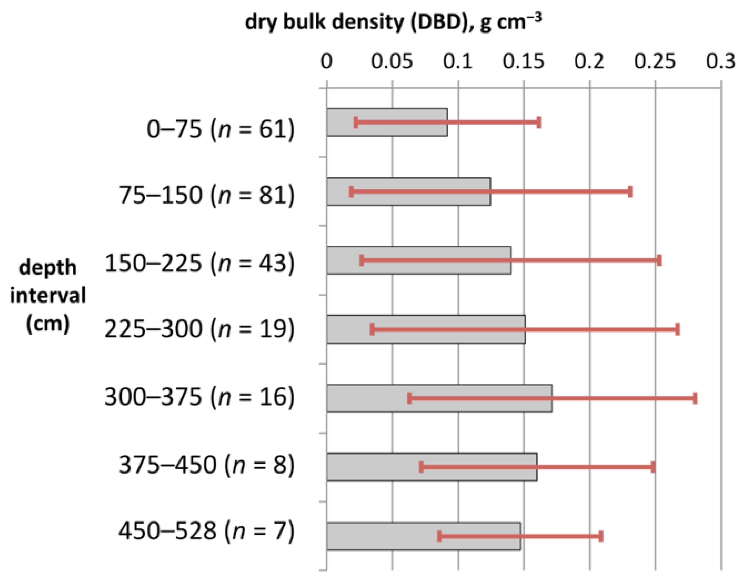
3.3. Assessing Patterns in DBD

Dry bulk density values are non-normally distributed with a 0.404 maximum. Each DBD value has a discrete depth and the correction equation yields a dataset showing a very mild increase with depth (simple least squares R² = 0.132). This corrected data set can be seen in Figure 5. The absolute ranges of densities exhibited at 68 cm and again at the 151 cm corrected depths are markedly low (0.0357 and 0.0224 g cm⁻³, respectively). Prompted by this result, we separated DBD values into 75 cm intervals (Figure 6). Relating these DBD values to the measured OM percentages creates three subsamples of comparable size after pooling the 150–225 cm and 225–300 cm intervals. Each interval also achieves 0.695 ± 0.05 R² values for power-law with intercept models related to their densities; in each case, they were greater than those calculated for logarithmic (Table 3, see also Figure 7). Additionally, despite the large variation in k1 per site, the k1′s for each interval all fall close to 0.04 g cm⁻³ with consistency (Table 4).

4. Discussion

Rudiyanto et al. [9] imply that any tropical peat sample with DBD greater than 0.25 g cm⁻³ is likely very clayey: past a point of utility in predicting wider trends of carbon storage. Samples that exceed 0.25 g cm⁻³, as seen in Figure 5, may allow us to distinguish the effects of clay intrusion: that they are transient and not reliant on any consistent depth. These cases do not conform to a simple increase with depth and can be seen at various depths. Note that these outliers do not represent the termination of cores in clay-heavy basement layers, as evidenced by their commonality throughout corrected depths. The low correlation of density with depth indicates that Amazonian peatland soils are unpredictable in their density at the landscape scale. Moreover, when paired with the nonlinear relationship between OM and DBD, they support a view of peatlands possessing belowground landscapes of varying densities that have implications for biotic processes at or near the surface. That general linear models show close to p = 0.05 significance levels for the interaction of the depth factor gives us reason to believe that the transient influence of high-density soil describes a past process of peat burial.

Since this is the second case of Amazonian peatlands presenting this pattern, we expect many Amazonian peatlands to present is as well, given sufficient sampling. Unlike in Bhomia et al. [20], our data come from a much deeper range of depths, at least ruling out the “>30 cm” category they detected. Depth values appear to be central to the variation in OM and DBD (Figure 2), as opposed to any relatable trend of depth with lower OM. Specific drawbacks of the analysis presented in Bhomia et al. [20] are secondary to the overt drop in the quality of the evidence supporting logarithmic models in the current study. We caution against tacit application of logarithms in this context.

A simple explanation for the non-linear relationship is that mineral intrusion over time causes discontinuity in the soil. Confirmation of the relationship may simply be illustrating a process that is recapitulated in other soil types, but over much longer time scales. Jeffrey [11] states that it might be universal. The process of pedogenesis in Amazonian peatlands, being so dynamic and sensitive to hydrologic perturbations, suggests that a wider variety of mathematical models may be more applicable. It must be noted that this is not the case in the well-studied Indonesian peatlands system, where the prevalence of ombrotrophic domes [4,5,55,56,57] suggests the ecosystems are regularly cut off from hydrologic influence [58]. The lack of reports of a nonlinear decay of OM with DBD is in keeping with the theory laid down by Adams [59], who observed that the relationship breaks down beyond 70% OM. Indonesian peatlands regularly average well above 50% OM [8,9,60,61], and difficulty in drawing out the pattern is to be expected with high OM data sets.

Although our OM numbers represent a wide range of percentages both above and below a 40% threshold, they are empirically low compared to measurements from other tropical peatlands. This would seem to at least call into question the 65% criteria used in Dargie et al. [39] or corroborate the 50% threshold used in Hastie et al. [7]. This lower bracket for OM in Amazonian peatlands was unexpected, and the selection process for loss on ignition was not comprehensive against the complete 200-plus sample collection. In the future it could be advisable to prioritize LOI over other analyses, as it would have increased our total sample size, addressing poor support for some statistics (e.g., site-based). We hope we have demonstrated that LOI assessment can drive multiple analyses moving forward. Although peatland studies are mostly directed at soils rich in organic matter, high-density samples should not be neglected. Detailed investigation on the exact composition of mineral-laden soils in Amazonian peatlands should be sought in future studies. Additionally, while logistical challenges may limit coring capacity in the field, we recommend that future studies still make an effort to sample to 150 cm. In our study, the data would not show any notable results until a full 75 cm depth was taken into account. Not only does this better encompass patterns, but it also dampens sampling errors that are likely present in our datasets. Furthermore, in agreement with past studies, the volume-limiting step should be taken in the field [2,3]. Physical manipulation of samples may limit the detection of relationships indicative of ecosystemic processes or bias readings towards high OM. While Russian peat sampling is the best means, this step can be accomplished with inexpensive rings, tubes, or fixed coring equipment [62,63]. In so doing, many of the drawbacks of the current study owing to low sample size could be remedied.

Given low sample size, our findings with regard to the ideal mixing model are highly unstable, but they are in accordance with the theory [64,65]. Site 9 is the only site for which decreasing k1 does not incur a concomitant increase in k2, and for which notable clay layers or changes in density where not observed at sites with greater than −0.3 g cm⁻³ k2. Overall, the negative k2 values are representative of profoundly organic soils, as expected for peat. While Morris et al. [40] utilized the k1 coefficient in explaining accretion, the behavior of k2 among sites may be more instructive to ecosystem processes. However, the k1 results should be considered indicative of greater organic contribution at sites 2 and 13 compared to the other heavily sampled site 10. That these k1 values trend with the x-intercept values garnered from general linear models further supports the deeply organic state of the peat at those sites, but the overall trends speak toward the possibility of distinguishing sites in which greater organic inputs may be occurring.

Morris et al. [40] state that site-based estimates of k1 were inappropriate given the ranges of organic matter that some sites occupied, with some going well below the 40% threshold (mean 30%, 12% minimum). By focusing on Amazonian peatlands, we did not face this limitation. To test if a majority of Amazonian peatlands also conform to a similar range, a wider scale of OM would need to be established with more intense sampling spatially and with a greater number of sites. Proceeding to estimates of accretion is problematic, with so few studies being able to state accumulation rates in Amazonian peatlands [31,66], and no volumetric mass accretion can be rendered from their methods. At the same time, our maximum k1 being roughly the same as the minimum detected in Morris et al. [40] (0.05 g cm⁻³) would seem to predict negligible rates of accretion. This, when paired with the negative k2 values, generally validates the application of the ideal mixing model to Amazonian peatlands.

In the coastal wetlands studied by Morris et al. [42], mineral inputs involved in accretion occurred daily, and are much easier to quantify [67,68,69]. In Amazonian peatlands, similar inputs are attenuated over annual flood pulses [23,70], but may be incurring a similar process of accretion, i.e., increase in soil layer thickness, as the ecosystem receives them at or near the soil surface [16,26,28,29,30,31,32,33]. Thus, better quantification of OM relationships may be able to diagnose higher rates of peat accumulation in certain peatlands, or wider peatland systems (i.e., interregional variation). Although not as precise, this approach should be less time-consuming than detailed elemental analysis studies, and much less expensive than isotopic methods. We suggest a means to at least allow for land managers and conservationists to develop a scheme that feeds directly into protection strategies for peatlands. Considering tropical peatlands’ significance to the global carbon pool, this should be a high priority for future research [27,71,72,73,74].

5. Conclusions

We present some soil characteristics from peatlands in the central Peruvian Amazon. The presence of a non-linear relationship between organic matter and dry bulk density prompted further exploration of relationships, highlighting information on potential ecosystem processes. In general, the modeling we applied does not uphold logarithmic models. While R² values support power-law with intercept decrease tendency, AIC provides further support for the ideal mixing model: a model that predicts accretion in North American coastal wetlands. We suggest further use of the ideal mixing model to attempt to distinguish higher rates of peat accumulation in some peatlands, and the revision of organic matter thresholds indicative of peat to lower levels.

References

1. Kolka, R.; Sebestyen, S.; Verry, E.S.; Brooks, K. Peatland Biogeochemistry and Watershed Hydrology at the Marcell Experimental Forest; CRC Press: Boca Raton, FL, USA, 2011. [Google Scholar]
2. Chimner, R.A.; Ott, C.A.; Perry, C.H.; Kolka, R.K. Developing and Evaluating Rapid Field Methods to Estimate Peat Carbon. Wetlands 2014, 34, 1241–1246. [Google Scholar] [CrossRef]
3. Chambers, F.M.; Beilman, D.; Yu, Z. Methods for Determining Peat Humification and for Quantifying Peat Bulk Density, Organic Matter and Carbon Content for Palaeostudies of Climate and Peatland Carbon Dynamics. Mires Peat 2011, 7, 1–10. [Google Scholar]
4. Minasny, B.; Berglund, Ö.; Connolly, J.; Hedley, C.; de Vries, F.; Gimona, A.; Kempen, B.; Kidd, D.; Lilja, H.; Malone, B. Digital Mapping of peatlands—A Critical Review. Earth-Sci. Rev. 2019, 196, 102870. [Google Scholar] [CrossRef]
5. Jaenicke, J.; Rieley, J.O.; Mott, C.; Kimman, P.; Siegert, F. Determination of the amount of carbon stored in Indonesian peatlands. Geoderma 2008, 147, 151–158. [Google Scholar] [CrossRef]
6. Page, S.E.; Rieley, J.O.; Banks, C.J. Global and regional importance of the tropical peatland carbon pool. Glob. Change Biol. 2011, 17, 798–818. [Google Scholar] [CrossRef]
7. Hastie, A.; Coronado, E.N.H.; Reyna, J.; Mitchard, E.T.A.; Åkesson, C.M.; Baker, T.R.; Cole, L.E.S.; Oroche, C.J.C.; Dargie, G.; Dávila, N.; et al. Risks to carbon storage from land-use change revealed by peat thickness maps of Peru. Nat. Geosci. 2022, 15, 369–374. [Google Scholar] [CrossRef]
8. Warren, M.W.; Kauffman, J.B.; Murdiyarso, D.; Anshari, G.; Hergoualc’H, K.; Kurnianto, S.; Purbopuspito, J.; Gusmayanti, E.; Afifudin, M.; Rahajoe, J.; et al. A cost-efficient method to assess carbon stocks in tropical peat soil. Biogeosciences 2012, 9, 4477–4485. [Google Scholar] [CrossRef]
9. Rudiyanto, R.; Minasny, B.; Setiawan, B.I. Further results on comparison of methods for quantifying soil carbon in tropical peats. Geoderma 2016, 269, 108–111. [Google Scholar] [CrossRef]
10. Grigal, D.F.; Brovold, S.L.; Nord, W.S.; Ohmann, L.F. Bulk Density of Surface Soils and Peat in the North Central United States. Can. J. Soil Sci. 1989, 69, 895–900. [Google Scholar] [CrossRef]
11. Jeffrey, D.W. A Note on the use of Ignition Loss as a Means for the Approximate Estimation of Soil Bulk Density. J. Ecol. 1970, 58, 297–299. [Google Scholar] [CrossRef]
12. Périé, C.; Ouimet, R. Organic carbon, organic matter and bulk density relationships in boreal forest soils. Can. J. Soil Sci. 2008, 88, 315–325. [Google Scholar] [CrossRef]
13. Sequeira, C.H.; Wills, S.A.; Seybold, C.A.; West, L.T. Predicting soil bulk density for incomplete databases. Geoderma 2014, 213, 64–73. [Google Scholar] [CrossRef]
14. Vasques, G.M.; Grunwald, S.; Comerford, N.B.; Sickman, J.O. Regional modelling of soil carbon at multiple depths within a subtropical watershed. Geoderma 2010, 156, 326–336. [Google Scholar] [CrossRef]
15. Yi, X.; Li, G.; Yin, Y. Pedotransfer Functions for Estimating Soil Bulk Density: A Case Study in the Three-River Headwater Region of Qinghai Province, China. Pedosphere 2016, 26, 362–373. [Google Scholar] [CrossRef]
16. Upton, A.; Vane, C.H.; Girkin, N.; Turner, B.L.; Sjögersten, S. Does Litter Input Determine Carbon Storage and Peat Organic Chemistry in Tropical Peatlands? Geoderma 2018, 326, 76–87. [Google Scholar] [CrossRef]
17. Quesada, C.A.; Paz, C.; Mendoza, E.O.; Phillips, O.L.; Saiz, G.; Lloyd, J. Variations in soil chemical and physical properties explain basin-wide Amazon forest soil carbon concentrations. Soil 2020, 6, 53–88. [Google Scholar] [CrossRef]
18. Wiese, L.; Ros, I.; Rozanov, A.; Boshoff, A.; de Clercq, W.; Seifert, T. An approach to soil carbon accounting and mapping using vertical distribution functions for known soil types. Geoderma 2016, 263, 264–273. [Google Scholar] [CrossRef]
19. Vepraskas, M.J.; Craft, C.B. Wetland Soils: Genesis, Hydrology, Landscapes, and Classification; CRC Press: Boca Raton, FL, USA, 2016. [Google Scholar]
20. Bhomia, R.K.; van Lent, J.; Rios, J.M.G.; Hergoualc’H, K.; Coronado, E.N.H.; Murdiyarso, D. Impacts of Mauritia flexuosa degradation on the carbon stocks of freshwater peatlands in the Pastaza-Marañón river basin of the Peruvian Amazon. Mitig. Adapt. Strat. Glob. Change 2018, 24, 645–668. [Google Scholar] [CrossRef]
21. Kalliola, R.; Salo, J.; Puhakka, M.; Rajasilta, M.; Häme, T.; Neller, R.; Räsänen, M.; Arias, W.D. Upper amazon channel migration. Naturwissenschaften 1992, 79, 75–79. [Google Scholar] [CrossRef]
22. Lähteenoja, O.; Reátegui, Y.R.; Räsänen, M.; Torres, D.D.C.; Oinonen, M.; Page, S. The Large Amazonian Peatland Carbon Sink in the Subsiding Pastaza-Marañón Foreland Basin, Peru. Glob. Change Biol. 2012, 18, 164–178. [Google Scholar] [CrossRef]
23. Junk, W.J.; Piedade, M.T.F.; Schöngart, J.; Cohn-Haft, M.; Adeney, J.M.; Wittmann, F. A Classification of Major Naturally-Occurring Amazonian Lowland Wetlands. Wetlands 2011, 31, 623–640. [Google Scholar] [CrossRef]
24. Aniceto, K.; Moreira-Turcq, P.; Cordeiro, R.C.; Quintana, I.; Fraizy, P.; Turcq, B. Hydrological Changes in West Amazonia over the Past 6 Ka Inferred from Geochemical Proxies in the Sediment Record of a Floodplain Lake. Procedia Earth Planet. Sci. 2014, 10, 287–291. [Google Scholar] [CrossRef]
25. Räsänen, M.; Neller, R.; Salo, J.; Jungner, H. Recent and ancient fluvial deposition systems in the Amazonian foreland basin, Peru. Geol. Mag. 1992, 129, 293–306. [Google Scholar] [CrossRef]
26. Lähteenoja, O.; Page, S. High Diversity of Tropical Peatland Ecosystem Types in the Pastaza-Marañón Basin, Peruvian Amazonia. J. Geophys. Res. Biogeosciences 2011, 116, G02025. [Google Scholar] [CrossRef]
27. Lawson, I.T.; Kelly, T.J.; Aplin, P.; Boom, A.; Dargie, G.; Draper, F.C.H.; Hassan, P.N.Z.B.P.; Hoyos-Santillan, J.; Kaduk, J.; Large, D.J.; et al. Improving estimates of tropical peatland area, carbon storage, and greenhouse gas fluxes. Wetl. Ecol. Manag. 2014, 23, 327–346. [Google Scholar] [CrossRef]
28. Limpens, J.; Berendse, F.; Blodau, C.; Canadell, J.G.; Freeman, C.; Holden, J.; Roulet, N.; Rydin, H.; Schaepman-Strub, G. Peatlands and the carbon cycle: From local processes to global implications—A synthesis. Biogeosciences 2008, 5, 1475–1491. [Google Scholar] [CrossRef]
29. Neue, H.; Gaunt, J.; Wang, Z.; Becker-Heidmann, P.; Quijano, C. Carbon in tropical wetlands. Geoderma 1997, 79, 163–185. [Google Scholar] [CrossRef]
30. Pastor, J.; Peckham, B.; Bridgham, S.; Weltzin, J.; Chen, J. Plant Community Dynamics, Nutrient Cycling, and Alternative Stable Equilibria in Peatlands. Am. Nat. 2002, 160, 553–568. [Google Scholar] [CrossRef]
31. Kelly, T.J.; Lawson, I.T.; Roucoux, K.H.; Baker, T.R.; Jones, T.D.; Sanderson, N.K. The vegetation history of an Amazonian domed peatland. Palaeogeogr. Palaeoclim. Palaeoecol. 2017, 468, 129–141. [Google Scholar] [CrossRef]
32. Blodau, C. Carbon cycling in peatlands—A review of processes and controls. Environ. Rev. 2002, 10, 111–134. [Google Scholar] [CrossRef]
33. Sjögersten, S.; Cheesman, A.W.; Lopez, O.; Turner, B.L. Biogeochemical processes along a nutrient gradient in a tropical ombrotrophic peatland. Biogeochemistry 2010, 104, 147–163. [Google Scholar] [CrossRef]
34. Smith, N.D.; Cross, T.A.; Dufficy, J.P.; Clough, S.R. Anatomy of an avulsion. Sedimentology 1989, 36, 1–23. [Google Scholar] [CrossRef]
35. Morozova, G.S.; Smith, N.D. Organic matter deposition in the Saskatchewan River floodplain (Cumberland Marshes, Canada): Effects of progradational avulsions. Sediment. Geol. 2003, 157, 15–29. [Google Scholar] [CrossRef]
36. Treat, C.C.; Kleinen, T.; Broothaerts, N.; Dalton, A.S.; Dommain, R.; Douglas, T.A.; Drexler, J.Z.; Finkelstein, S.A.; Grosse, G.; Hope, G.; et al. Widespread global peatland establishment and persistence over the last 130,000 y. Proc. Natl. Acad. Sci. USA 2019, 116, 4822–4827. [Google Scholar] [CrossRef]
37. Dubroeucq, D.; Volkoff, B. From Oxisols to Spodosols and Histosols: Evolution of the soil mantles in the Rio Negro basin (Amazonia). CATENA 1998, 32, 245–280. [Google Scholar] [CrossRef]
38. Junk, W.J.; Furch, K. A general review of tropical South American floodplains. Wetl. Ecol. Manag. 1993, 2, 231–238. [Google Scholar] [CrossRef]
39. Dargie, G.C.; Lewis, S.L.; Lawson, I.T.; Mitchard, E.T.A.; Page, S.E.; Bocko, Y.E.; Ifo, S.A. Age, extent and carbon storage of the central Congo Basin peatland complex. Nature 2017, 542, 86–90. [Google Scholar] [CrossRef]
40. Morris, J.T.; Barber, D.C.; Callaway, J.C.; Chambers, R.; Hagen, S.C.; Hopkinson, C.S.; Johnson, B.J.; Megonigal, P.; Neubauer, S.C.; Troxler, T.; et al. Contributions of organic and inorganic matter to sediment volume and accretion in tidal wetlands at steady state. Earth’s Future 2016, 4, 110–121. [Google Scholar] [CrossRef]
41. Villa, J.A.; Bernal, B. Carbon sequestration in wetlands, from science to practice: An overview of the biogeochemical process, measurement methods, and policy framework. Ecol. Eng. 2018, 114, 115–128. [Google Scholar] [CrossRef]
42. Dirección de Gestión del Territorio, Autoridad Reigonal Ambiental de Ucayali. Estudio De Clima Y Zonas De Vida. In Zonificacion Ecologica y Economica de la Region Ucayali; Dirección de Gestión del Territorio, Autoridad Reigonal Ambiental de Ucayali: Ucayali, Peru, 2016; pp. 1–64. [Google Scholar]
43. Sanchez Huaman, S.; Torres, L.C.; Llamocca Huamani, J. Ucayali: Sinergias Por El Clima; Centro de Conservación Investigación y Manejo de Áreas Naturales: Lima, Peru, 2017; p. 25. [Google Scholar]
44. Dirección de Gestión del Territorio, Autoridad Reigonal Ambiental de Ucayali. Suelos Y Capacidad De Uso Mayor De Las Tierras. In Zonificacion Ecologica y Economica de la Region Ucayali; Dirección de Gestión del Territorio, Autoridad Reigonal Ambiental de Ucayali: Ucayali, Peru, 2016; 181p. [Google Scholar]
45. Quesada, C.A.; Phillips, O.L.; Schwarz, M.; Czimczik, C.I.; Baker, T.R.; Patiño, S.; Fyllas, N.M.; Hodnett, M.G.; Herrera, R.; Almeida, S.; et al. Basin-wide variations in Amazon forest structure and function are mediated by both soils and climate. Biogeosciences 2012, 9, 2203–2246. [Google Scholar] [CrossRef]
46. Nascimento, N.R.D.; Fritsch, E.; Bueno, G.T.; Bardy, M.; Grimaldi, C.; Melfi, A.J. Podzolization as a deferralitization process: Dynamics and chemistry of ground and surface waters in an Acrisol—Podzol sequence of the upper Amazon Basin. Eur. J. Soil Sci. 2008, 59, 911–924. [Google Scholar] [CrossRef]
47. de Assis, R.L.; Wittmann, F.; Bredin, Y.K.; Schöngart, J.; Quesada, C.A.N.; Piedade, M.T.F.; Haugaasen, T. Above-ground woody biomass distribution in Amazonian floodplain forests: Effects of hydroperiod and substrate properties. For. Ecol. Manag. 2019, 432, 365–375. [Google Scholar] [CrossRef]
48. Goulding, M.; Cañas, C.; Barthem, R.; Forsberg, B.; Ortega, H. Amazon Headwaters: Rivers, Wildlife, and Conservation in Southeastern Peru; Asociacion para la Conservacion de la Cuenca Amazonica, ACCA: Lima, Peru, 2003; p. 117. [Google Scholar]
49. García-Soria, D.; Honorio-Coronado, E.N.; Del Castillo-Torres, D. Determinación del Stock de Carbono en Aguajales de la Cuenca del Río Aguaytía, Ucayali—Perú. Folia Amaz. 2012, 21, 153–160. [Google Scholar] [CrossRef]
50. Junk, W.J.; Piedade, M.T.; Wittmann, F.; Schöngart, J.; Parolin, P. Amazonian Floodplain Forests: Ecophysiology, Biodiversity and Sustainable Management; Springer: Dordrecht, The Netherlands, 2010; p. 618. [Google Scholar]
51. Jowsey, P.C. An Improved Peat Sampler. New Phytol. 1966, 65, 245–248. [Google Scholar] [CrossRef]
52. R Core Team. R: A Language and Environment for Statistical Computing; R Foundation for Statistical Computing: Vienna, Austria, 2018. [Google Scholar]
53. Bates, D.; Mächler, M.; Bolker, B.; Walker, S. Fitting Linear Mixed-Effects Models using Lme4. arXiv 2014, arXiv:1406.5823. [Google Scholar]
54. Elzhov, T.V.; Mullen, K.M.; Spiess, A.; Bolker, B. R Package, Version 1.1-8; Minpack.Lm: R Interface to the Levenberg-Marquardt Nonlinear Least-Squares Algorithm found in MINPACK, Plus Support for Bounds; R Core: R Foundation for Statistical Computing: Vienna, Austria, 2013. [Google Scholar]
55. Hergoualc’H, K.; Verchot, L.V. Stocks and fluxes of carbon associated with land use change in Southeast Asian tropical peatlands: A review. Glob. Biogeochem. Cycles 2011, 25, GB2001. [Google Scholar] [CrossRef]
56. Hooijer, A.; Page, S.; Canadell, J.G.; Silvius, M.; Kwadijk, J.; Wösten, H.; Jauhiainen, J. Current and future CO2 emissions from drained peatlands in Southeast Asia. Biogeosciences 2010, 7, 1505–1514. [Google Scholar] [CrossRef]
57. Konecny, K.; Ballhorn, U.; Navratil, P.; Jubanski, J.; Page, S.E.; Tansey, K.; Hooijer, A.; Vernimmen, R.; Siegert, F. Variable carbon losses from recurrent fires in drained tropical peatlands. Glob. Change Biol. 2016, 22, 1469–1480. [Google Scholar] [CrossRef]
58. Ingram, H.A.P. Size and shape in raised mire ecosystems: A geophysical model. Nature 1982, 297, 300–303. [Google Scholar] [CrossRef]
59. Adams, W.A. The Effect of Organic Matter on the Bulk and True Densities of Some Uncultivated Podzolic Soils. Eur. J. Soil Sci. 1973, 24, 10–17. [Google Scholar] [CrossRef]
60. Farmer, J.; Matthews, R.; Smith, P.; Langan, C.; Hergoualc’H, K.; Verchot, L.; Smith, J.U. Comparison of methods for quantifying soil carbon in tropical peats. Geoderma 2014, 214, 177–183. [Google Scholar] [CrossRef]
61. Page, S.E.; Rieley, J.O.; Shotyk, W.; Weiss, D. Interdependence of Peat and Vegetation in a Tropical Peat Swamp Forest. Philos. Trans. R. Soc. Lond. B Biol. Sci. 1999, 354, 1885–1897. [Google Scholar] [CrossRef] [PubMed]
62. De Vleeschouwer, F.; Chambers, F.M.; Swindles, G.T. Coring and Sub-Sampling of Peatlands for Palaeoenvironmental Research. Mires Peat 2010, 7, 1–10. [Google Scholar]
63. US Forest Service. Forest Inventory and Analysis, US. Soil measurements and sampling. In Field Methods for Forest Health (Phase 3) Measurements; US Forest Service, Ed.; US Forest Service: Logan, UT, USA, 2011; pp. 1–29. [Google Scholar]
64. Federer, C.A.; Turcotte, D.E.; Smith, C.T. The organic fraction–bulk density relationship and the expression of nutrient content in forest soils. Can. J. For. Res. 1993, 23, 1026–1032. [Google Scholar] [CrossRef]
65. Stewart, V.; Adams, W.; Abdulla, H. Quantitative Pedological Studies on Soils Derived from Silurian Mudstones: II. the Relationship between Stone Content and the Apparent Density of the Fine Earth. J. Soil Sci. 1970, 21, 248–255. [Google Scholar] [CrossRef]
66. Roucoux, K.H.; Lawson, I.T.; Jones, T.D.; Baker, T.R.; Jones, T.D.; Gosling, W.D.; Lähteenoja, O. Vegetation development in an Amazonian peatland. Palaeogeogr. Palaeoclim. Palaeoecol. 2013, 374, 242–255. [Google Scholar] [CrossRef]
67. Davis, J.L.; Currin, C.A.; O’Brien, C.; Raffenburg, C.; Davis, A. Living Shorelines: Coastal Resilience with a Blue Carbon Benefit. PLoS ONE 2015, 10, e0142595. [Google Scholar] [CrossRef]
68. Neubauer, S.C. Contributions of mineral and organic components to tidal freshwater marsh accretion. Estuar. Coast. Shelf Sci. 2008, 78, 78–88. [Google Scholar] [CrossRef]
69. Morris, J.T.; Bowden, W.B. A Mechanistic, Numerical Model of Sedimentation, Mineralization, and Decomposition for Marsh Sediments 1. Soil Sci. Soc. Am. J. 1986, 50, 96–105. [Google Scholar] [CrossRef]
70. Furch, K.; Junk, W.J. Physicochemical Conditions in the Floodplains. In The Central Amazon Floodplain; Junk, W.J., Ed.; Springer: Berlin/Heidelberg, Germany, 1997; pp. 69–108. [Google Scholar] [CrossRef]
71. Roucoux, K.H.; Lawson, I.T.; Baker, T.R.; Del Castillo Torres, D.; Draper, F.C.; Lähteenoja, O.; Gilmore, M.P.; Honorio Coronado, E.N.; Kelly, T.J.; Mitchard, E.T.A. Threats to intact tropical peatlands and opportunities for their conservation. Conserv. Biol. 2017, 31, 1283–1292. [Google Scholar] [CrossRef]
72. Posa, M.R.C.; Wijedasa, L.S.; Corlett, R.T. Biodiversity and Conservation of Tropical Peat Swamp Forests. Bioscience 2011, 61, 49–57. [Google Scholar] [CrossRef]
73. Leifeld, J.; Menichetti, L. The underappreciated potential of peatlands in global climate change mitigation strategies. Nat. Commun. 2018, 9, 1071. [Google Scholar] [CrossRef] [PubMed] [Green Version]
74. Sjögersten, S.; de la Barreda-Bautista, B.; Brown, C.; Boyd, D.; Lopez-Rosas, H.; Hernández, E.; Monroy, R.; Rincón, M.; Vane, C.; Moss-Hayes, V.; et al. Coastal wetland ecosystems deliver large carbon stocks in tropical Mexico. Geoderma 2021, 403, 115173. [Google Scholar] [CrossRef]
Figure 1. Major road and waterways in Ucayali and surrounding departments in central Peru (UTM 18S)—yellow stars are sites included in this study.
Sustainability 14 12070 g001
Figure 2. Scatterplot of organic matter percentage by dry bulk density: Note position of reddish-grey points, which exceed the mean of sample-specific depths (152 cm), and extreme depths in red.
Sustainability 14 12070 g002
Figure 3. Logarithmic generalized linear mixed model displaying lines for each site, with overall fit in red; normality among residuals W = 0.982, p = 0.304, AIC = −295.4, marginal R2 = 0.896.
Sustainability 14 12070 g003
Figure 4. Scatter plots of individual sites 4 (left) and 5 (right).
Sustainability 14 12070 g004
Figure 5. DBD measurements corrected to the 220 cm third quartile of all sample depths: dashed line shows the 0.25 g cm−3 cutoff identified by Rudiyanto et al. [9] as indicative of clayey composition.
Sustainability 14 12070 g005
Figure 6. 95% confidence intervals for average dry bulk densities in each 75 cm depth interval.
Sustainability 14 12070 g006
Figure 7. OM to DBD data subset restricted from 150–300 cm empirical depth: the logarithmic model DBD = −0.266 ln(OM) − 0.103 has R2 = 0.659, and the AIC = −71.26 (n = 20).
Sustainability 14 12070 g007