Article

Analysis of Decadal Land Use Changes and Its Impacts on Urban Heat Island (UHI) Using Remote Sensing-Based Approach: A Smart City Perspective

1
Punjab Remote Sensing Centre, Ludhiana 141004, India
2
Department of Climate Change and Agricultural Meteorology, Punjab Agricultural University, Ludhiana 141004, India
3
Department of Water Resources Development and Management, Indian Institute of Technology Roorkee, Roorkee 247667, India
4
Department of Geography, Panjab University, Chandigarh 160014, India
5
Department of Civil, Environmental and Natural Resources Engineering, Lulea University of Technology, 971 87 Lulea, Sweden
*
Authors to whom correspondence should be addressed.
Sustainability 2022, 14(19), 11892; https://doi.org/10.3390/su141911892
Submission received: 17 June 2022 / Revised: 25 August 2022 / Accepted: 18 September 2022 / Published: 21 September 2022

Abstract

:
The land surface temperature (LST) pattern is regarded as one of the most important indicators of the environmental consequences of land use/land cover change. The possible contribution of land surface to the warming phenomenon is being investigated by scientists across the world. This research focuses on variations in surface temperature and urban heat islands (UHIs) over the course of two seasons, i.e., winter and summer. Using remotely sensed datasets and geospatial techniques, an attempt was made to analyze the spatiotemporal variation in urban heat islands (UHIs) and its association with LULC over Chandigarh from 2000 to 2020. The Enhanced Built-up and Bareness Index (EBBI), Dry Built-up Index (DBI), and Dry Bare-Soil Index (DBSI) were used to identify built-up areas in the city. The results revealed an increase of 10.08% in BA, whereas the vegetation decreased by 4.5% over the study period, which is in close agreement with the EBBI, DBI, and DBSI assessments. From 2000 to 2020, the UHI intensities increased steadily in both the summer and winter seasons. Dense built-up areas such as the industrial unit of the city possessed the highest UHIindex (>0.7) values.

1. Introduction

Land use and land cover (LULC) changes significantly influence land surface temperature (LST), which is a crucial indicator of the earth’s environmental condition. LST positively impacts terrestrial biophysical processes such as plant respiration, evapotranspiration, and photosynthesis. The influence of LULC changes on climate is predominantly due to urban expansion, which impacts biogeochemical cycles such as hydrological and nutrient cycles, as well as natural ecosystems and biodiversity. Since 1990, many studies have been carried out on LST retrieval using thermal remote sensing [1,2,3,4,5,6,7,8]. The urban heat island (UHI) refers to the temperature difference between urban and non-urban rural areas [9,10,11,12,13]. The changes in the land surface due to urbanization, which rapidly increases the impervious land covers and leads to a surge in sensible heat flux, are the main cause of the UHI phenomenon. Rapid population growth has evolved in economic and industrial developments that have gradually transformed the natural environment into urbanized regions with severely polluted air and densely built-up areas. Therefore, research on urban environments has gained significant attention in recent decades. Pal and Ziaul [14] employed satellite remote sensing to study the land surface temperature in relation to vegetation conditions characterized by the normalized difference vegetation index (NDVI). They observed the highest temperature (29.97 °C) in settlement areas and the lowest (18.58 °C) in a water body. Therefore, understanding the dynamic LULC systems is critical not just for LST and LULC change research [14] but also for social, economic, and environmental concerns. As the population increases, a city tends to expand its territory, resulting in changes in LULC patterns and an increase of several degrees in average temperature over the surrounding undeveloped areas, which significantly impacts the UHI structure. The LULC pattern modifications can also happen naturally due to floods, droughts, earthquakes, etc. City planners in tropical and sub-tropical countries that are quickly developing are concerned about the rising temperatures. UHI is most evident in these cities, particularly in the summer and winter seasons.
Remote sensing and geographic information system (GIS) techniques have been utilized efficiently in several environmental and hydrometeorological applications [15,16,17,18,19,20,21,22,23,24,25,26]. These techniques can be used to study the changes in LULC patterns and their impact on both temperature and hydrological alterations [27,28,29,30,31,32,33,34]. The regional climate has been influenced by recent changes in metropolitan areas, which have been reported to be more abrupt and quick in recent decades [35,36,37,38]. The LST or surface skin temperature is affected by three factors: the urban architecture, the kind of land cover, and the thermal and radiative properties of the surface [39,40]. Basically, LST refers to how hot or cool the surface feels in a certain region. The temperature of the ground surface is always different from the temperature of the air. Indices like NDVI were used to distinguish between barren lands and built-up areas from vegetated areas and aquatic bodies when mapping land cover types. Surawar and Kotharkar [41] employed Landsat 7 Enhanced Thematic Mapper plus (ETM+) images to investigate the influence of LULC changes on LST and its impact on UHI development in Nagpur, India. Their findings revealed a significant reduction in vegetation cover due to the continuous expansion of built-up areas. The intensity of UHI in Nagpur increased by 0.7 °C between 2000 and 2006, which increased more than twofold (1.8 °C) between 2006 and 2013. Investigation of surface UHI in the Indian city Punjab using MODIS-LST products (spatial resolution 1000 m) disclosed that the temperature fluctuation inside the built-up area and its surroundings, which could be attributed to the differences in land use, and the downscaled LST depicts better results compared to the original image [42]. Zheng [43] updated the standard split-window approach to recover LST using Sentinel-3A SLSTR data, and they concluded that LST can be estimated with greater than 1 K accuracy. Kafy et al. [44] determined the variation in LULC and its effects on the urban thermal environment, such as LST, UHI, and urban field variance index (UTFVI) for Chattogram, Bangladesh. They employed multi-temporal Landsat Thematic Mapper (TM) and Operational Land Imager (OLI) satellite images to classify LULC classes in different years (1999, 2009, and 2019) and identified the transition between different LULCs, and corresponding changes in LST, UHI, and UFVI. Rasool et al. [45] used remote sensing imageries to study LULC change in the Kashmir Himalaya during 1990, 2002, and 2017 using Landsat-5 TM, Landsat-7 ETM+, and Landsat-8 OLI data. The results identified a continuous reduction in cropland and expansion of horticulture. During the 27-year study period, the total cropland loss was 278 km2 (5% of the total area) (19.80% cropland) with a minor reduction in forests (54 m2), while horticulture expanded from 176 km2 (3.2%) in 1990 to 409 km2 (7.49%) in 2017. The built-up area increased from 133 km2 in 1990 to 208 km2 in 2002 and 313 km2 in 2017. Ramaiah et al. [46] assessed the impact of urbanization on LST in two traditional Indian cities, Panaji and Tumkur, which are being suggested for development as smart cities. They utilized the Landsat data-derived spectral indices such as the Enhanced Built-up and Bareness Index (EBBI), Modified Normalized Difference Water Index (MNDWI), and Soil Adjusted Vegetation Index (SAVI) to characterize the green cover and built-up areas. According to the multivariate regression model, Tumkur’s adjusted R2 value was 0.716 with a standard error of 1.97, whereas the adjusted R2 value for Panaji was 0.698 with a standard error of 1.407. Polydoros et al. [47] quantified the trends in LST and surface UHI intensity in Mediterranean Cities in terms of Smart Urbanization and found positive LST trends in metropolitan locations, particularly at night, ranging from +0.412 °K in Marseille to +0.923 °K in Cairo. They observed an increase in SUHI over the past 18 years, particularly during the daytime in Mediterranean cities such as Rome (+0.332 °K) and Barcelona (+0.307 °K).
In this study, indices such as the Dry Built-up Index (DBI), EBBI, and Dry Bare-Soil Index (DBSI) are computed to discern between barren land and built-up areas effectively. This study focused primarily on the analysis of the LST and assessed the impact of LST on the UHI patterns and its variations over the last 20 years over an Indian smart city during the summer and winter seasons.

2. Study Area

Chandigarh city, situated on the Trans Indo-Gangetic plain, was selected as the study area. The city covers an area of approximately 114 km2 with an average elevation of 321 m (1053 ft). The location of the city is presented in Figure 1. The city experiences five seasons, i.e., spring, summer, monsoon, autumn, and winter. The summer temperature usually ranges from 40 °C to 42 °C, but the maximum value reaches 44 °C. The typical winter temperatures range between −1 °C and 14 °C. According to the Census of India 2011, Chandigarh has a population of 1,055,450, i.e., a density of about 9252 persons per km2. The urban population accounts for 97.25% of the overall population. The southern part of Chandigarh city has the highest population density. The city’s main government offices are in the north, while the industrial regions are in the southeast, separated from the residential parts by a greenbelt filled with mango trees [48,49,50].

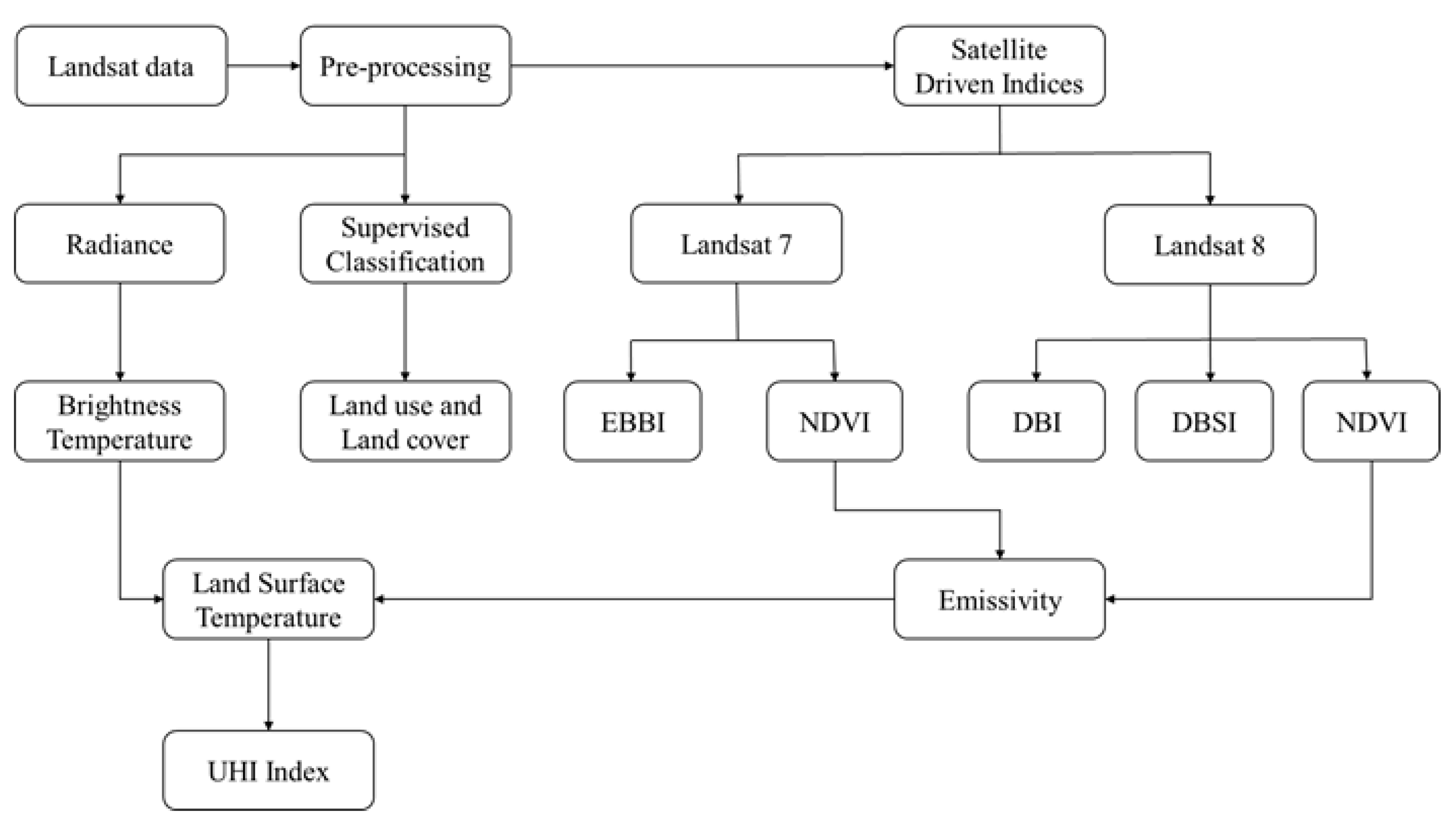
3. Data and Methodology

3.1. Satellite Data Pre-Processing

Landsat 7 ETM+ and Landsat 8 OLI images were used in 10-year intervals to determine the distributions of LST and urban heat island areas in summer and winter during 2000–2020 for Chandigarh city. The images were obtained from the United States Geological Survey (USGS) Earth Explorer user interface. The band details of Landsat 7 and 8 were found at Landsat Science (https://landsat.gsfc.nasa.gov, accessed on 15 January 2022). Table 1 lists the specifics of the data that are used in this study. The image pre-processing techniques were applied to the images as layer stacking and masking using the study area boundary. The multi-spectral bands such as visible, near-infrared, and shortwave infrared were used to identify the LULC classes and generate spectral indices. The LST was retrieved using brightness temperature from the thermal bands and NDVI from visual and NIR bands. Figure 2 depicts the retrieval process of LST and UHI.

3.2. LULC Extraction and Change Analysis

There are a variety of methods that can be utilized to implement supervised classification; however, in this research, ERDAS IMAGINE software (Stockholm, Sweden) was utilized with the commonly used maximum likelihood classifier (MLC). Different spectral signatures of Landsat images were found and matched to Google Earth images from the same time period to classify Chandigarh into five key LULC classes: Dense Vegetation (DV), Crop or Grass Lands (CGL), Dry/Barren Lands (BL), Water Bodies (WB), Built-up Areas (BU). Band composition was performed on Landsat 7 and Landsat 8 OLI images prior to classification of LULC classes. Bands 1 to 5 and band 7 composition Landsat was performed for Landsat 7, and bands 1 to 7 composition was performed for Landsat 8. The composite bands for three years were then used as input parameters to run the maximum likelihood classifier. The main advantage of using parametric algorithms such as MLC is their ease of use. Parametric approaches are more useful and easier to implement for non-complex terrains with clearly defined LULC categories.
The PA assesses the accuracy of a classification scheme by calculating the proportion of correct classifications for a given class, whereas the UA determines the chance that a class into which a given pixel in an image is classified truly represents that class [51,52]. The ratio of properly classified reference points to the total reference points is regarded as the overall accuracy. On the other hand, the Kappa coefficient considers both incorrectly and correctly classified pixels to provide a more reliable estimate of accuracy than the overall accuracy.

3.3. Derivation of Spectral Indices

The spectral indices, i.e., NDVI, EBBI, DBI, and DBSI, were calculated. The formulas used to compute the different spectral indices are given in Table 2. According to a recent study by Li et al. [53], EBBI is useful for identifying built-up areas and bare ground cover. Thus, we employed the EBBI index to separate the built-up and barren land combinedly to understand the land cover and LST alteration due to human-induced activities. The EBBI generated for Landsat 7 images with radiometric resolutions of 8 bits (256 grey levels) is ineffective for Landsat 8 images with radiometric resolutions of 16 bits (4096 grey levels). Thus, DBI and DBSI were derived using the Landsat 8 imagery as suggested by Rasul [54].

3.4. Retrieval of Land Surface Temperature (LST) Using Plank Inversion Model

Brightness temperature (TB) and emissivity (ε) are the precursors for the LST estimation. The spectral radiance (Lλ) can be retrieved by conversion of digital numbers (DN) of thermal bands using Equation (1) [55,56].
T B = K 2 ln [ ( K 1 L λ ) + 1 ]
where K1 and K2 are band-specific calibration constants for Landsat.
L λ = [ L m a x L m i n 255 1 ]   ( Q C A L 1 ) + L min
where Lλ is the spectral radiance, and Q C A L is the thermal band.
Further, the NDVI Thresholds Method was used to measure emissivity (ε) [57,58].
ε = εvPv + εs(1 − Pv) + dε
where Pv is fractional vegetation given by
P v = [ N D V I N D V I m i n N D V I m a x N D V I m i n ]
εv = 0.987 and εs = 0.972 and dε is the surface geometry.

3.5. Urban Heat Island Index (UHIindex)

The changes in UHI are derived using the LST pattern. The UHIindex is determined using the following equation [59]:
U H I I n d e x = L S T i L S T m i n L S T m a x L S T m i n
where LSTi is the value of LST in the image, and LSTmax and LSTmin are the maximum and minimum LST values, respectively.

4. Results

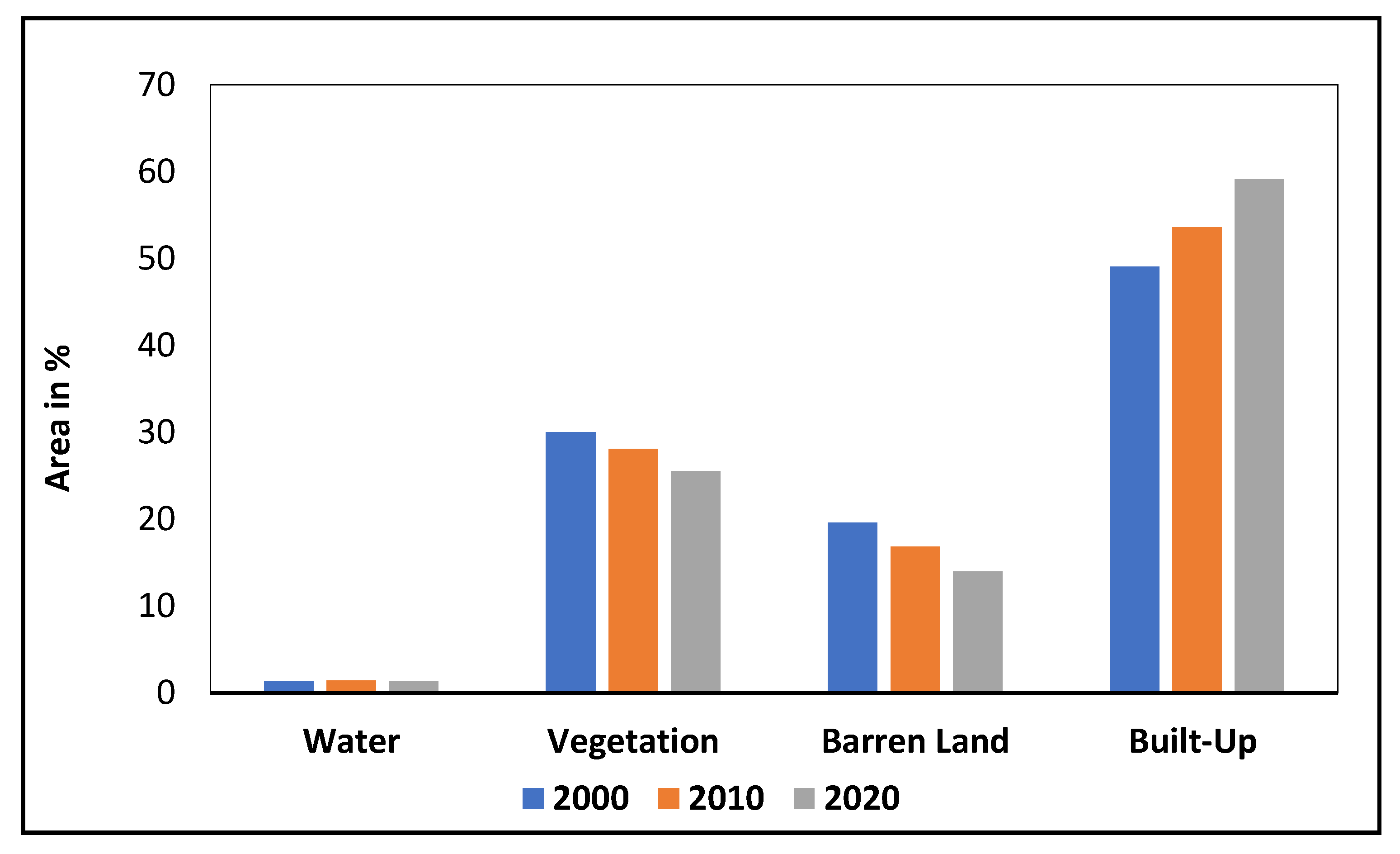
4.1. LULC Classification

The highest overall classification accuracy (88%) was obtained for 2020, followed by 2000 (84%) and 2010 (82%), which indicates an acceptable accuracy range (Table 3). Similarly, the highest kappa value was observed for 2020 (0.81), followed by 2000 (0.77) and 2010 (0.74). The classified maps for different years are shown in Figure 3.

4.2. Decadal LULC Change Analysis

Significant changes in the area have been identified for the different LULC classes during the observation period. The built-up area has increased remarkably during the study period, and the spatial changes are shown in Figure 3. The built-up area covering 49.04% in 2000 increased to 53.58% in 2010 and 59.12% in 2020 (Table 4; Figure 4). The vegetated areas showed a 1.9% decrease from 2000 to 2010 and then a 2.6% decrease from 2010 to 2020 with respect to the total study area. Similarly, barren land coverage with respect to the study area has been continuously decreasing in the 20-year duration, and the gross reduction is 5.67%. In contrast, the built-up areas have shown the maximum increase from 2000 to 2020, i.e., an expansion of more than 10% of the area of the city. The area of water bodies in the city has been nearly the same over the decades. Most of the settlement area increases are observed at the expense of barren land followed by cropland. Such conversions are primarily observed in the peripheral regions of the city.

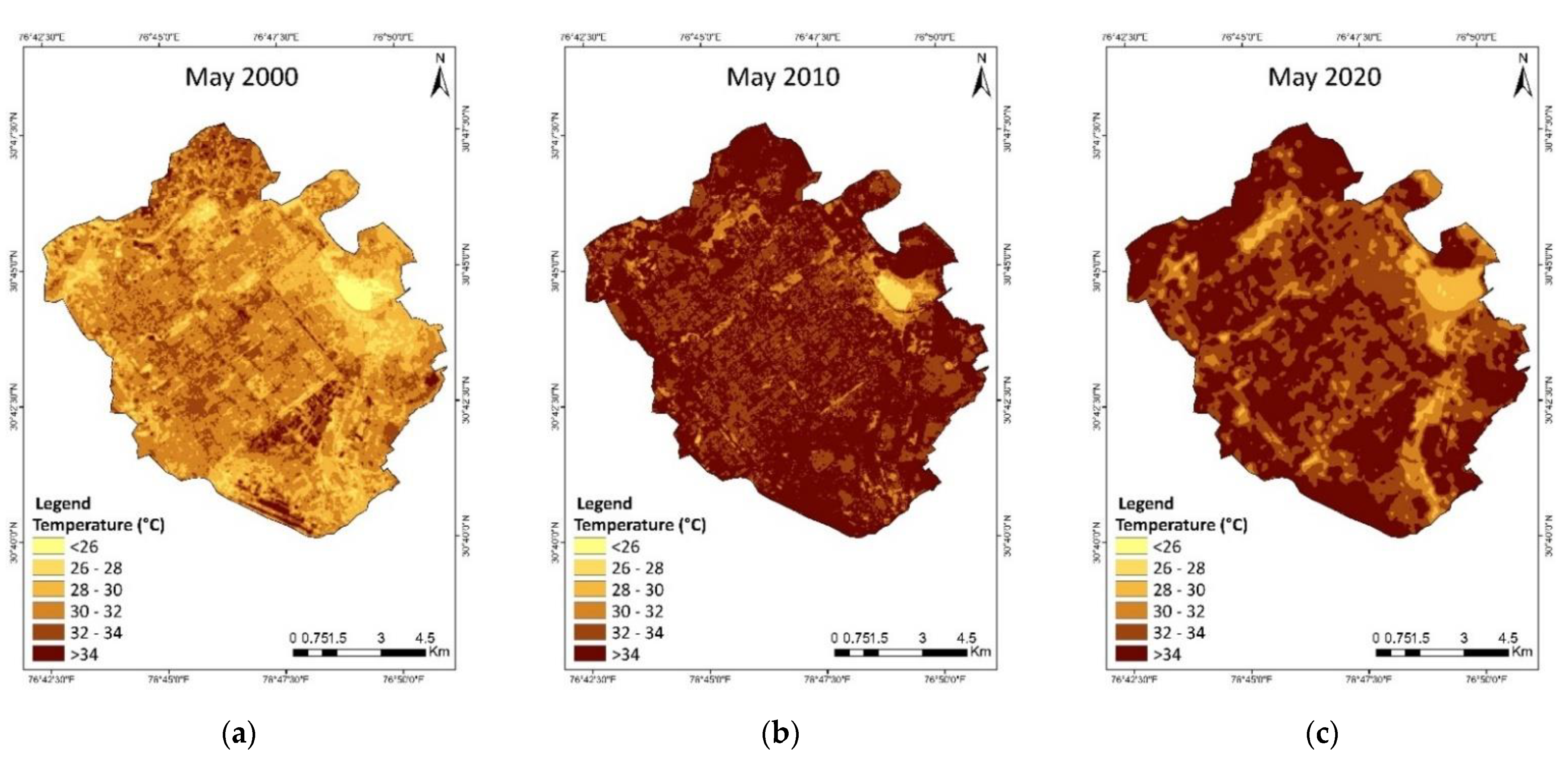
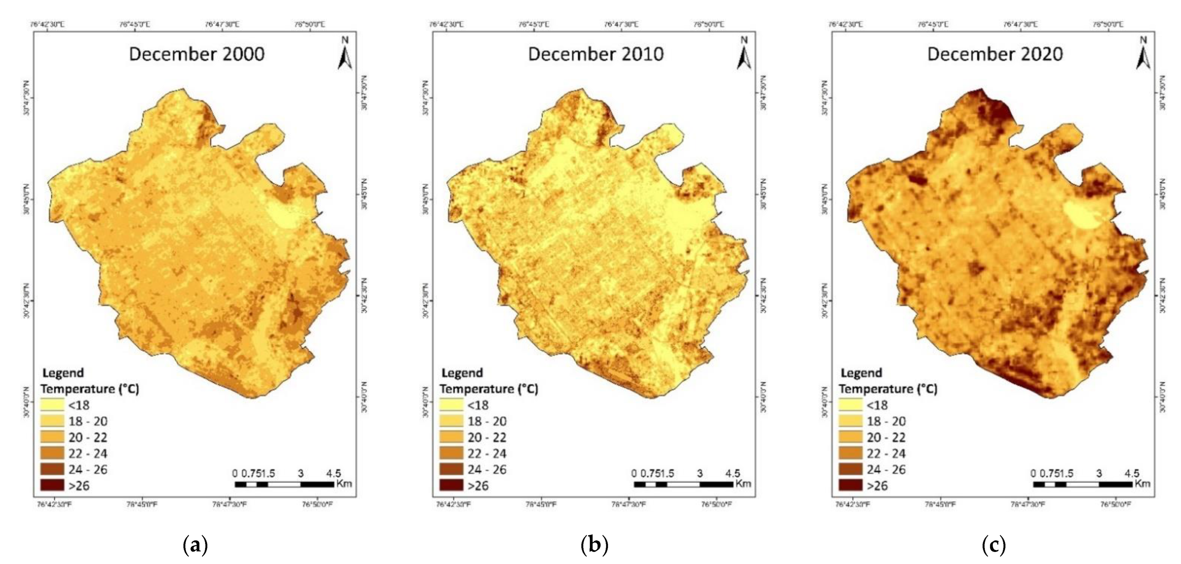
4.3. Spatio-Temporal Distribution of LST during Summer and Winter

Figure 5 and Figure 6 depict the LST distributions for both seasons. The LST for the summer season was 22 °C to 43 °C, whereas it was 10 °C to 28 °C during the winter.
  • Summer: It has been noticed that the LST ranges over the city have risen from 21–36 °C to 26–42 °C in two decades. The highest LST values are observed over built-up areas and bare lands. More specifically, the highest LST is identified over the industrial area and barren land on the city’s borders. In comparison, lower LST values are observed in vegetated areas.
  • Winter: The LST ranges have also risen during the winter season from 13–22 °C in 2000 to 17–28 °C in 2020. During the winter season, a similar LST distribution pattern to the summer season is observed with the difference in LST values.

4.4. LST Distribution Pattern for Different LULC Classes

Figure 7 depicts the average distribution of LST in both seasons for different LULC classes. During summer, the built-up area possessed the highest LST for all the years. However, in the winter season, the average LST of barren land is higher than that of all other LULC classes. The vegetation class showed the lowest temperature in both seasons for all the years.

4.5. Differentiation of Built-Up (BU) Area and Barren Land (BL) Using DBSI, DBI, and EBBI

The DBSI and DBI are calculated from the Landsat 8 images; however, Landsat 7 is used for the calculation of EBBI. Figure 8 shows the DBI and DBSI maps during both seasons in 2020. The higher DBI values depict the BU, whereas the moderate values dictate BL in the image. In the case of DBSI, the high values depict BL, compared to the moderate values, which indicate BU areas.
However, the regions with the highest and the lowest values of DBSI vary in May and December over the agricultural areas in the northern parts of the city. This could be attributed to the Zaid crop growing month of May, whereas December is the near-harvest period of the Kharif season crop (Figure 8). The highest DBSI values are found in the periphery region, which depicts the BL, and the moderate values are observed in the BU areas, located in the central part of the city. Comparatively lower values of DBSI in the map depict the vegetation and water body.
Figure 9 shows the EBBI distribution for 2000 and 2010 (summer and winter), where the BL may be found in the city’s outlying regions with the highest EBBI range values, while the BU can be found in the city’s center with moderate values. The lower values are used to identify vegetation and water bodies.

4.6. Seasonal Variation of Remote Sensing Indices through Correlation Study

Correlation among the different spectral indices and LST is established for both seasons to understand the variations in the LST better. Figure 10 depicts the correlation coefficient values among the different indices.

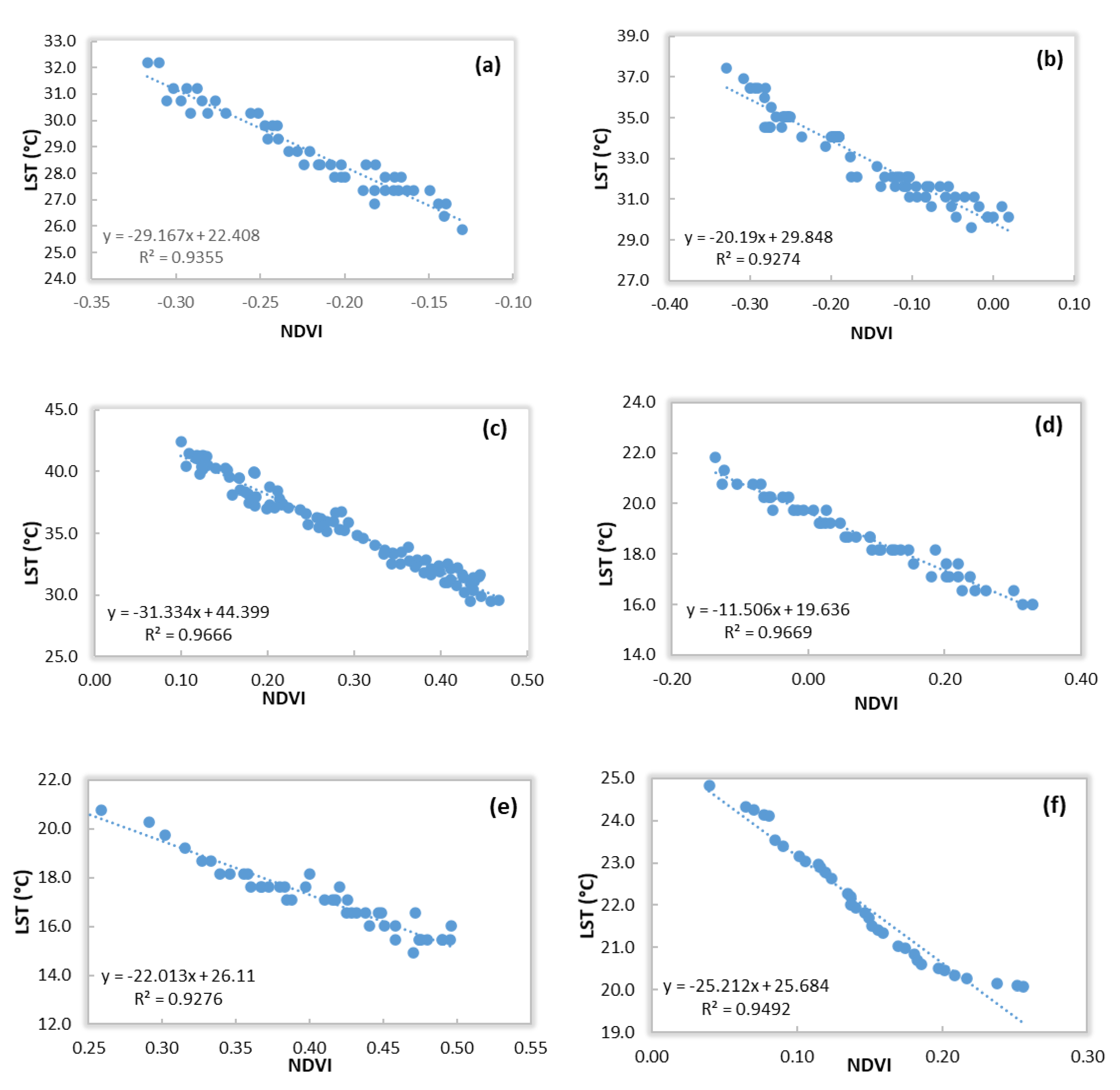
4.7. Relationship between NDVI and Land Surface Temperature

Figure 11 shows scatter plots indicating the interaction between NDVI and LST for both the seasons of 2000, 2010, and 2020. The low NDVI values depict the BU and BL, whereas the positive values are found to be higher in vegetated areas. A strong negative relation is found between the NDVI and LST for all the years. The coefficient of determination is found to be more than 0.92. Figure 12 depicts the class-wise distribution of LST for different years.

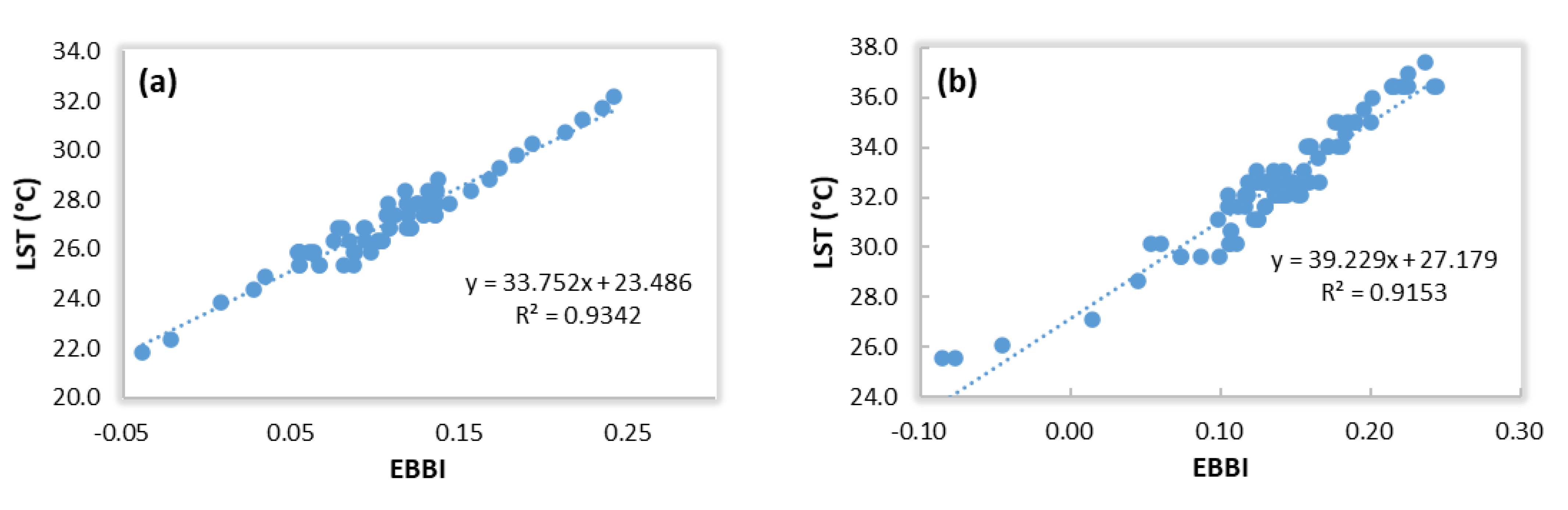
4.8. Relationship between Land Surface Temperature and EBBI

Figure 13 shows the scatter plot of LST and EBBI for both the seasons during 2000 and 2010. The BL is indicated by high EBBI values, while the BU is indicated by lower values. A strong positive relationship is observed between EBBI and LST, where LST increases with increasing EBBI values. The coefficient of determination between LST and EBBI is found to be more than 0.91 for both summer and winter.

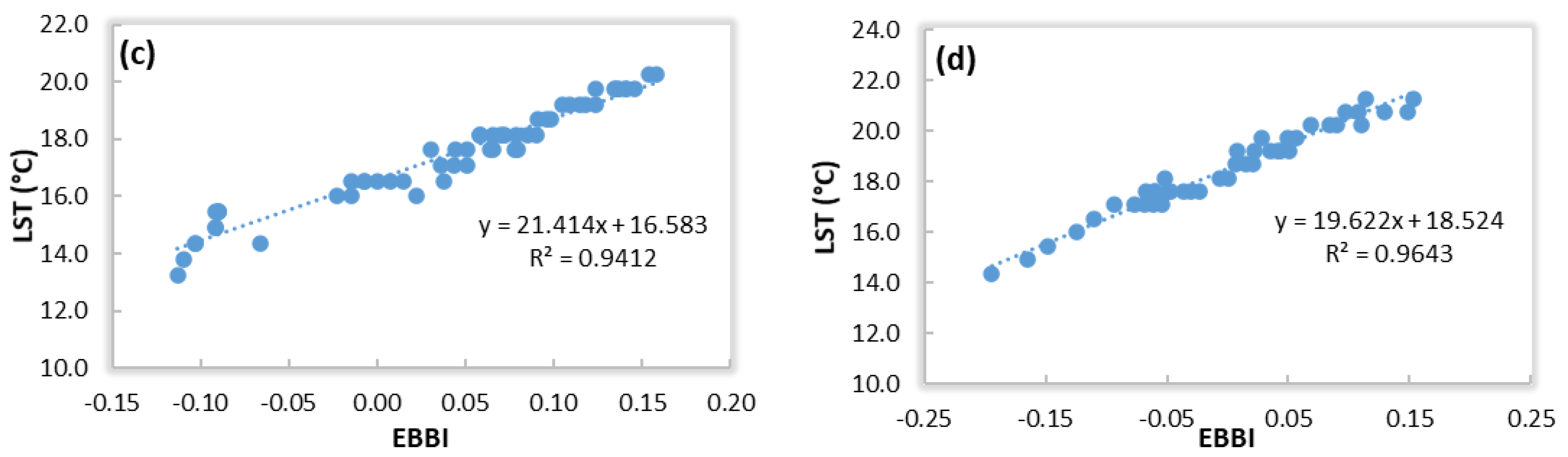
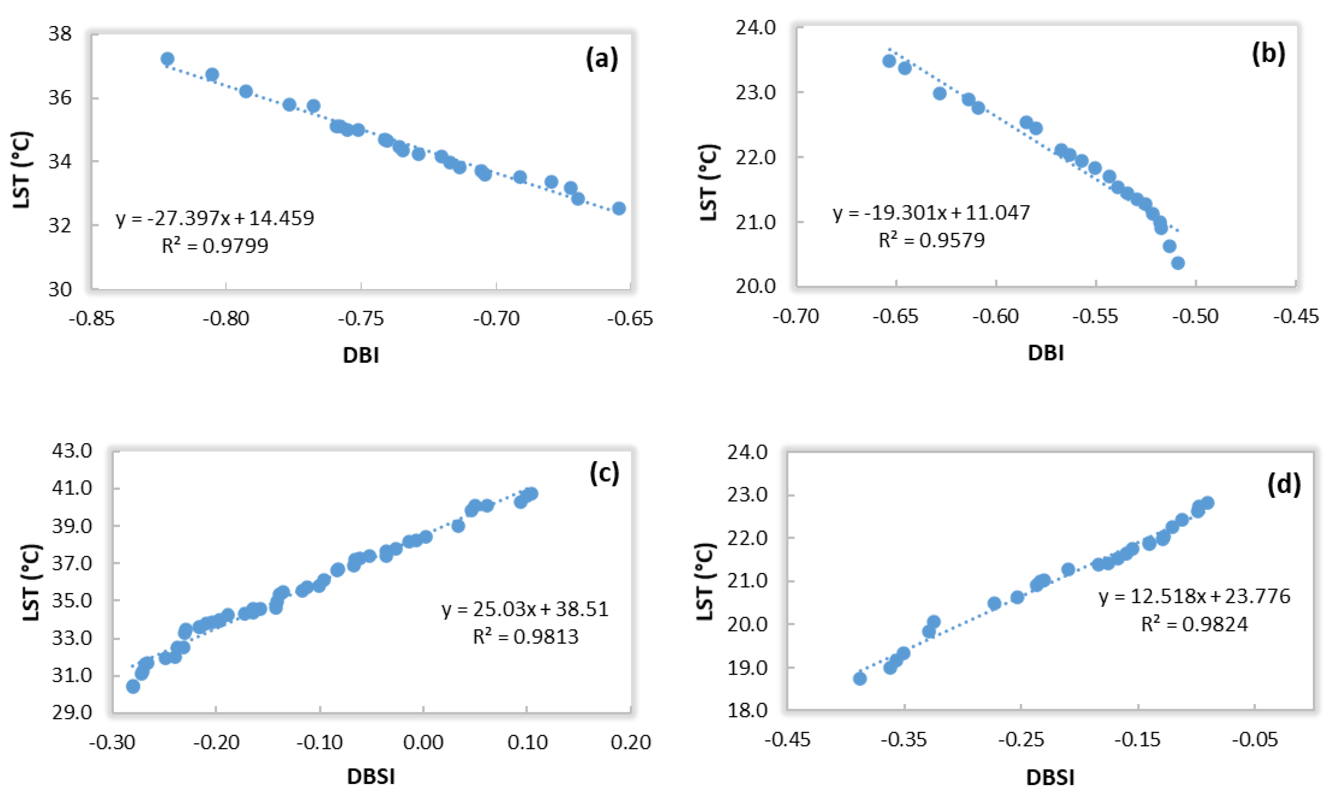
4.9. Relationship between DBI, DBSI, and LST

Figure 14 depicts the relationship of LST with DBI and DBSI for both seasons in 2020. A strong negative relationship is observed between DBI and LST. The higher values of DBI are observed for BU, whereas the lower values are observed for BL. On the other hand, the DBSI shows an opposite relationship (i.e., strong positive) with LST, wherein the higher values are observed for BL than BU. The coefficient of determination is more than 0.95 between LST and DBI, while it is more than 0.98 between DBSI and LST.

4.10. Identification of Urban Heat Island Index (UHIindex)

It has been noted that the BL, BU, and industrial regions had greater LST than other LULC categories; these little pockets of higher temperature are known as UHIs. The UHIindex was calculated for each satellite image. The average UHIindex for both seasons is calculated by taking the mean of the individual UHIindex for the summer and winter seasons. UHIindex values were 0.5 to 0.7 in the summer for the BU at the center of the city, whereas they were 0.7 or higher in the south-eastern zone of the industrial area, as shown in Figure 15. The UHIindex values in the vegetated regions varied between 0.3 and 0.6, with a few exceptions. Table 5 depicts the difference in different UHI classes for both seasons.

4.11. Average UHIindex over 20 Years

The lower average UHI values are found in a large water body (Sukhna Lake) present on the north-eastern side of the city, indicating no significant heating (Figure 16). However, the average UHI values increased in settlement areas where sparse settlement areas have been converted into dense settlement areas. Due to the presence of industries, the southern side of the city possessed a strong UHI zone. The average UHI map depicts the areas associated with higher or lower UHI zones created throughout the city.

5. Discussion

The recent IPCC report [60] suggests that climate change adaptation is essential to build climatic resilience and achieve sustainable development goals (SDGs). It is challenging to assess the impact of urbanization on climate and environment, specifically to identify the future needs and the key aspects towards enhancing climatic resilience [61]. The use of comprehensive technological measures can limit the increase in mean temperature and achieve the SDGs for the cities/urban areas. Implementing climate change adaptation and mitigation strategies, e.g., reducing emissions, building disaster resilient frameworks, and nature-based solutions, etc., is essential for achieving the SDGs. Studying the land use changes in the past decades and their impact on UHI is needed of the hour, and it is pertinent to SDG 11 and SDG 13 [42].
The continuous developments and rapid population growth in Chandigarh city in the past couple of decades have resulted rapid BU expansion (i.e., above 10% area of the city) by replacing the barren lands and vegetation. BU and BL areas are found to have higher LST ranges compared to vegetation and water bodies. In previous investigations, similar outcomes were reported in various cities [62,63,64]. LST has gradually increased from May 2000 to 2020. The LST in May 2000 is mostly estimated between 26 °C and 32 °C, which increased in 2010, wherein most of the area in the city had a temperature of more than 34 °C. In 2020, the central part of the city recorded a temperature between 32 to 34 °C. Again, the peripheral regions of the city possessed a temperature of more than 34 °C. The south-eastern part containing the industrial area and airport region always had a LST of more than 34 °C throughout the study period. The LST gradually increased in the winter season also from 2000 to 2020. The average LST of the city increased from 18–22 °C to 20–24 °C. The temperature in the peripheral regions of the city in 2020 was recorded as more than 26 °C. The decadal LULC change analysis has identified the major conversions as bare land and agricultural land into settlement areas. Such conversions have led to increased LST and UHI.
The BL has been identified throughout Chandigarh, with hotspots (highest concentration) in the city’s northern outskirts. Also, it is observed that more areas at the periphery of the city possessed higher LST during summer as compared to winter. Due to the lack of vegetation and water surface, dense settlement areas, including the industrial areas, possessed higher LST throughout our study period in both seasons. Due to the overlapping NDVI value ranges, vegetation spectral indices such as NDVI cannot distinguish between BU and BL areas [65]. On the contrary, spectral indices such as DBSI, DBI, and EBBI were included to effectively identify the BU and BL, and their contribution to LST. A strong negative correlation is observed for LST with NDVI and DBI, whereas LST has a strong positive correlation with EBBI and DBSI. High UHIindex values (>0.7) were observed during both seasons, mostly over the industrial and dense settlement areas and BL. These regions indicate the UHIs of the city. From 2000 to 2020, the intensity of surface urban heat was greater in May than in December, which can be mostly ascribed to the intensity and duration of direct solar irradiance, lower rainfall events, and air temperature. The longer available solar hours in May than in December heat the land surface more in May than in December.
The current study uses the Landsat thermal band, which has a 60 m and 100 m spatial resolution. However, higher-resolution satellite data could provide better results to determine the effect of urban vegetation and urbanization on the LST distribution. Future studies may attempt the formation of the surface materials and their differential contribution to LST. In this study, we have retrieved the LST and its spatial distribution, demarcated it in Chandigarh city, and analyzed the UHI. The generated LST, UHI, and green cover maps can help prescribe nature-based solutions to improve urban climate resilience [66].

6. Conclusions

Chandigarh has seen a rapid growth of urbanization, resulting in a fast expansion of settlement areas in the city (i.e., an increase of 10.08%). The overall accuracy of LULC classification is 82–88%. During both seasons, higher LST was observed mostly over the dense BU, BL, and industrial areas. LST has a strong negative association with NDVI and DBI in both seasons, with a coefficient of determination of more than 0.85. BL has higher EBBI values than BU, and there is a strong positive correlation between EBBI and LST, with a coefficient of determination of more than 0.85. The EBBI and DBSI have a positive relationship with LST. As the formation of UHIs leads to the alteration of the regional climate, the first step to taking appropriate mitigation measures is the identification of UHIs. In Chandigarh, BL, dense BU, and industrial areas are found to have higher UHIindex values as compared to green spaces and water bodies. Various mitigation strategies, such as green roofs, lighter-colored surfaces, etc., can be adopted to reduce the UHI effects.

Author Contributions

Conceptualization, S.S. (Sashikanta Sahoo), A.M. and S.S. (Sabyasachi Swain); methodology, S.S. (Sashikanta Sahoo), A.M. and S.S. (Sabyasachi Swain); software, S.S. (Sashikanta Sahoo) and A.M.; formal analysis, S.S. (Sashikanta Sahoo), A.M., S.S. (Sabyasachi Swain) and G.; data curation, A.M. and G.; writing—original draft preparation, S.S. (Sashikanta Sahoo), A.M. and S.S. (Sabyasachi Swain); writing—review and editing, G., B.P. and N.A.-A.; supervision, B.P. and N.A.-A.; project administration, S.S. (Sashikanta Sahoo) and B.P.; APC funding, N.A.-A. All authors have read and agreed to the published version of the manuscript.

Funding

This research received no external funding. The APC was funded by Lulea University, Sweden.

Institutional Review Board Statement

Not applicable.

Informed Consent Statement

Not applicable.

Data Availability Statement

Not applicable.

Acknowledgments

The authors acknowledge the open-access dataset provided by NASA and USGS, which is used in this study.

Conflicts of Interest

The authors declare no conflict of interest. The funders had no role in the design of the study; in the collection, analyses, or interpretation of data; in the writing of the manuscript, or in the decision to publish the results.

References

  1. Wan, Z.; Dozier, J. A generalized split-window algorithm for retrieving land-surface temperature from space. IEEE Trans. Geosci. Remote Sens. 1996, 34, 892–905. [Google Scholar]
  2. Gillespie, A.; Rokugawa, S.; Matsunaga, T.; Cothern, J.S.; Hook, S.; Kahle, A.B. A temperature and emissivity separation algorithm for Advanced Spaceborne Thermal Emission and Reflection Radiometer (ASTER) images. IEEE Trans. Geosci. Remote Sens. 1998, 36, 1113–1126. [Google Scholar] [CrossRef]
  3. Lakshmi, V.; Czajkowski, K.; Dubayah, R.; Susskind, J. Land surface air temperature mapping using TOVS and AVHRR. Int. J. Remote Sens. 2001, 22, 643–662. [Google Scholar] [CrossRef]
  4. Qin, Z.; Karnieli, A.; Berliner, P. A mono-window algorithm for retrieving land surface temperature from Landsat TM data and its application to the Israel-Egypt border region. Int. J. Remote Sens. 2001, 22, 3719–3746. [Google Scholar] [CrossRef]
  5. Aumann, H.H.; Chahine, M.T.; Gautier, C.; Goldberg, M.D.; Kalnay, E.; McMillin, L.M.; Revercomb, H.; Rosenkranz, P.W.; Smith, W.L.; Staelin, D.H.; et al. AIRS/AMSU/HSB on the Aqua mission: Design, science objectives, data products, and processing systems. IEEE Trans. Geosci. Remote Sens. 2003, 41, 253–264. [Google Scholar] [CrossRef]
  6. Ji, Z.; Jing, L.; Xiang, Z.; Wen-Feng, Z.; Jian-Xia, G. A modified single-channel algorithm for land surface temperature retrieval from HJ-1B satellite data. J. Infrared Millim. Waves 2011, 30, 61–67. [Google Scholar]
  7. Zhou, J.; Li, J.; Zhang, L.; Hu, D.; Zhan, W. Intercomparison of methods for estimating land surface temperature from a Landsat-5 TM image in an arid region with low water vapour in the atmosphere. Int. J. Remote Sens. 2012, 33, 2582–2602. [Google Scholar] [CrossRef]
  8. Liu, W.; Feddema, J.; Hu, L.; Zung, A.; Brunsell, N. Seasonal and diurnal characteristics of land surface temperature and major explanatory factors in Harris County, Texas. Sustainability 2017, 9, 2324. [Google Scholar] [CrossRef]
  9. Oke, T.R. City size and the urban heat island. Atmos. Environ. 1973, 7, 769–779. [Google Scholar] [CrossRef]
  10. Voogt, J.A.; Oke, T.R. Thermal remote sensing of urban climates. Remote Sens. Environ. 2003, 86, 370–384. [Google Scholar] [CrossRef]
  11. Voogt, J.A. Urban Heat Islands: Hotter Cities; ActionBioscience: Herndon, VA, USA, 2012. [Google Scholar]
  12. Rotach, M.W.; Vogt, R.; Bernhofer, C.; Batchvarova, E.; Christen, A.; Clappier, A.; Feddersen, B.; Gryning, S.E.; Martucci, G.; Mayer, H.; et al. BUBBLE–an urban boundary layer meteorology project. Theor. Appl. Climatol. 2005, 81, 231–261. [Google Scholar] [CrossRef]
  13. Roth, M. -Urban Heat Islands. In Handbook of Environmental Fluid Dynamics; CRC Press: Boca Raton, FL, USA, 2012; Volume 2, pp. 162–168. [Google Scholar]
  14. Pal, S.; Ziaul, S.K. Detection of land use and land cover change and land surface temperature in English Bazar urban centre. Egypt. J. Remote Sens. Space Sci. 2017, 20, 125–145. [Google Scholar] [CrossRef] [Green Version]
  15. Patel, P.; Thakur, P.K.; Aggarwal, S.P.; Garg, V.; Dhote, P.R.; Nikam, B.R.; Swain, S.; Al-Ansari, N. Revisiting 2013 Uttarakhand flash floods through hydrological evaluation of precipitation data sources and morphometric prioritization. Geomat. Nat. Hazards Risk 2022, 13, 646–666. [Google Scholar] [CrossRef]
  16. Swain, S.; Mishra, S.K.; Pandey, A.; Pandey, A.C.; Jain, A.; Chauhan, S.K.; Badoni, A.K. Hydrological modelling through SWAT over a Himalayan catchment using high-resolution geospatial inputs. Environ. Chall. 2022, 8, 100579. [Google Scholar] [CrossRef]
  17. Das, P.; Mudi, S.; Behera, M.D.; Barik, S.K.; Mishra, D.R.; Roy, P.S. Automated mapping for long-term analysis of shifting cultivation in Northeast India. Remote Sens. 2021, 13, 1066. [Google Scholar] [CrossRef]
  18. Swain, S.; Mishra, S.K.; Pandey, A.; Dayal, D. Spatiotemporal assessment of precipitation variability, seasonality, and extreme characteristics over a Himalayan catchment. Theor. Appl. Climatol. 2022, 147, 817–833. [Google Scholar] [CrossRef]
  19. Behera, M.D.; Gupta, A.K.; Barik, S.K.; Das, P.; Panda, R.M. Use of satellite remote sensing as a monitoring tool for land and water resources development activities in an Indian tropical site. Environ. Monit. Assess. 2018, 190, 401. [Google Scholar] [CrossRef]
  20. Swain, S.; Mishra, S.K.; Pandey, A.; Kalura, P. Inclusion of groundwater and socio-economic factors for assessing comprehensive drought vulnerability over Narmada River Basin, India: A geospatial approach. Appl. Water Sci. 2022, 12, 14. [Google Scholar] [CrossRef]
  21. Singh, K.V.; Setia, R.; Sahoo, S.; Prasad, A.; Pateriya, B. Evaluation of NDWI and MNDWI for assessment of waterlogging by integrating digital elevation model and groundwater level. Geocarto Int. 2015, 30, 650–661. [Google Scholar] [CrossRef]
  22. Gupta, A.; Himanshu, S.K.; Gupta, S.; Singh, R. Evaluation of the SWAT model for analyzing the water balance components for the upper Sabarmati Basin. Adv. Water Resour. Eng. Manag. 2020, 39, 141–151. [Google Scholar]
  23. Swain, S.; Taloor, A.K.; Dhal, L.; Sahoo, S.; Al-Ansari, N. Impact of climate change on groundwater hydrology: A comprehensive review and current status of the Indian hydrogeology. Appl. Water Sci. 2022, 12, 120. [Google Scholar] [CrossRef]
  24. Himanshu, S.K.; Pandey, A.; Yadav, B. Assessing the applicability of TMPA-3B42V7 precipitation dataset in wavelet-support vector machine approach for suspended sediment load prediction. J. Hydrol. 2017, 550, 103–117. [Google Scholar] [CrossRef]
  25. Aadhar, S.; Swain, S.; Rath, D.R. Application and performance assessment of SWAT hydrological model over Kharun river basin, Chhattisgarh, India. In ASCE World Environmental and Water Resources Congress 2019: Watershed Management, Irrigation and Drainage, and Water Resources Planning and Management; American Society of Civil Engineers: Reston, VA, USA, 2019; pp. 272–280. [Google Scholar]
  26. Himanshu, S.K.; Pandey, A.; Patil, A. Hydrologic evaluation of the TMPA-3B42V7 precipitation data set over an agricultural watershed using the SWAT model. J. Hydrol. Eng. 2018, 23, 05018003. [Google Scholar] [CrossRef]
  27. Palmate, S.S.; Amrit, K.; Jadhao, V.G.; Dayal, D.; Himanshu, S.K. Prioritization of erosion prone areas based on a sediment yield index for conservation treatments: A case study of the upper Tapi River basin. In Advances in Remediation Techniques for Polluted Soils and Groundwater; Elsevier: Amsterdam, The Netherlands, 2021; pp. 291–307. [Google Scholar]
  28. Himanshu, S.K.; Pandey, A.; Dayal, D. Evaluation of satellite-based precipitation estimates over an agricultural watershed of India. In ASCE World Environmental and Water Resources Congress 2018: Watershed Management, Irrigation and Drainage, and Water Resources Planning and Management; American Society of Civil Engineers: Reston, VA, USA, 2018; pp. 308–320. [Google Scholar]
  29. Swain, S.; Sahoo, S.; Taloor, A.K.; Mishra, S.K.; Pandey, A. Exploring recent groundwater level changes using Innovative Trend Analysis (ITA) technique over three districts of Jharkhand, India. Groundw. Sustain. Dev. 2022, 18, 100783. [Google Scholar] [CrossRef]
  30. Sahoo, S.; Swain, S.; Goswami, A.; Sharma, R.; Pateriya, B. Assessment of trends and multi-decadal changes in groundwater level in parts of the Malwa region, Punjab, India. Groundw. Sustain. Dev. 2021, 14, 100644. [Google Scholar] [CrossRef]
  31. Behera, M.D.; Murthy, M.S.R.; Das, P.; Sharma, E. Modelling forest resilience in Hindu Kush Himalaya using geoinformation. J. Earth Syst. Sci. 2018, 127, 95. [Google Scholar] [CrossRef]
  32. Das, P.; Behera, M.D.; Murthy, M.S.R. Forest fragmentation and human population varies logarithmically along elevation gradient in Hindu Kush Himalaya-utility of geospatial tools and free data set. J. Mt. Sci. 2017, 14, 2432–2447. [Google Scholar] [CrossRef]
  33. Swain, S.; Sahoo, S.; Taloor, A.K. Groundwater quality assessment using geospatial and statistical approaches over Faridabad and Gurgaon districts of National Capital Region, India. Appl. Water Sci. 2022, 12, 75. [Google Scholar] [CrossRef]
  34. Das, P.; Behera, M.D.; Pal, S.; Chowdary, V.M.; Behera, P.R.; Singh, T.P. Studying land use dynamics using decadal satellite images and Dyna-CLUE model in the Mahanadi River basin, India. Environ. Monit. Assess. 2019, 191, 804. [Google Scholar] [CrossRef]
  35. Guptha, G.C.; Swain, S.; Al-Ansari, N.; Taloor, A.K.; Dayal, D. Assessing the role of SuDS in resilience enhancement of urban drainage system: A case study of Gurugram City, India. Urban Clim. 2022, 41, 101075. [Google Scholar] [CrossRef]
  36. Yadav, B.; Gupta, P.K.; Patidar, N.; Himanshu, S.K. Ensemble modelling framework for groundwater level prediction in urban areas of India. Sci. Total Environ. 2020, 712, 135539. [Google Scholar] [CrossRef] [PubMed]
  37. Guptha, G.C.; Swain, S.; Al-Ansari, N.; Taloor, A.K.; Dayal, D. Evaluation of an urban drainage system and its resilience using remote sensing and GIS. Remote Sens. Appl. Soc. Environ. 2021, 23, 100601. [Google Scholar]
  38. Lwasa, S.; Mugagga, F.; Wahab, B.; Simon, D.; Connors, J.; Griffith, C. Urban and peri-urban agriculture and forestry: Transcending poverty alleviation to climate change mitigation and adaptation. Urban Clim. 2014, 7, 92–106. [Google Scholar] [CrossRef]
  39. Li, Z.L.; Tang, B.H.; Wu, H.; Ren, H.; Yan, G.; Wan, Z.; Trigo, I.F.; Sobrino, J.A. Satellite-derived land surface temperature: Current status and perspectives. Remote Sens. Environ. 2013, 131, 14–37. [Google Scholar] [CrossRef] [Green Version]
  40. Morabito, M.; Crisci, A.; Messeri, A.; Orlandini, S.; Raschi, A.; Maracchi, G.; Munafò, M. The impact of built-up surfaces on land surface temperatures in Italian urban areas. Sci. Total Environ. 2016, 551, 317–326. [Google Scholar] [CrossRef] [PubMed]
  41. Surawar, M.; Kotharkar, R. Assessment of urban heat island through remote sensing in Nagpur urban area using landsat 7 ETM+ Satellite Images. Int. J. Urban Civil Eng. 2017, 11, 868–874. [Google Scholar]
  42. Mukherjee, S.; Joshi, P.K.; Garg, R.D. Analysis of urban built-up areas and surface urban heat island using downscaled MODIS derived land surface temperature data. Geocarto Int. 2017, 32, 900–918. [Google Scholar] [CrossRef]
  43. Zheng, Y.; Ren, H.; Guo, J.; Ghent, D.; Tansey, K.; Hu, X.; Nie, J.; Chen, S. Land surface temperature retrieval from sentinel-3A sea and land surface temperature radiometer, using a split-window algorithm. Remote Sens. 2019, 11, 650. [Google Scholar] [CrossRef]
  44. Kafy, A.A.; Islam, M.; Sikdar, S.; Ashrafi, T.J.; Al-Faisal, A.; Islam, M.A.; Al Rakib, A.; Khan, M.H.H.; Sarker, M.H.S.; Ali, M.Y. Remote sensing-based approach to identify the influence of land use/land cover change on the urban thermal environment: A case study in Chattogram City, Bangladesh. In Re-Envisioning Remote Sensing Applications; CRC Press: Boca Raton, FL, USA, 2021; pp. 217–240. [Google Scholar]
  45. Rasool, R.; Fayaz, A.; ul Shafiq, M.; Singh, H.; Ahmed, P. Land use land cover change in Kashmir Himalaya: Linking remote sensing with an indicator based DPSIR approach. Ecol. Indic. 2021, 125, 107447. [Google Scholar] [CrossRef]
  46. Ramaiah, M.; Avtar, R.; Rahman, M.M. Land Cover Influences on LST in Two Proposed Smart Cities of India: Comparative Analysis Using Spectral Indices. Land 2020, 9, 292. [Google Scholar] [CrossRef]
  47. Polydoros, A.; Mavrakou, T.; Cartalis, C. Quantifying the Trends in Land Surface Temperature and Surface Urban Heat Island Intensity in Mediterranean Cities in View of Smart Urbanization. Urban Sci. 2018, 2, 16. [Google Scholar]
  48. Nimish, G.; Chandan, M.C.; Bharath, H.A. Understanding current and future landuse dynamics with land surface temperature alterations: A case study of Chandigarh. ISPRS Ann. Photogramm. Remote Sens. Spat. Inf. Sci. 2018, 4, 79–86. [Google Scholar] [CrossRef]
  49. Gupta, N.; Mathew, A.; Khandelwal, S. Analysis of cooling effect of water bodies on land surface temperature in nearby region: A case study of Ahmedabad and Chandigarh cities in India. Egypt. J. Remote Sens. Space Sci. 2019, 22, 81–93. [Google Scholar] [CrossRef]
  50. Mathew, A.; Sreekumar, S.; Khandelwal, S.; Kumar, R. Prediction of land surface temperatures for surface urban heat island assessment over Chandigarh city using support vector regression model. Sol. Energy 2019, 186, 404–415. [Google Scholar] [CrossRef]
  51. Sultana, S.; Satyanarayana, A.N.V. Urban heat island intensity during winter over metropolitan cities of India using remote-sensing techniques: Impact of urbanization. Int. J. Remote Sens. 2018, 39, 6692–6730. [Google Scholar] [CrossRef]
  52. Majumder, A.; Setia, R.; Kingra, P.K.; Sembhi, H.; Singh, S.P.; Pateriya, B. Estimation of land surface temperature using different retrieval methods for studying the spatiotemporal variations of surface urban heat and cold islands in Indian Punjab. Environ. Dev. Sustain. 2021, 23, 15921–15942. [Google Scholar] [CrossRef]
  53. Li, H.; Wang, C.; Zhong, C.; Su, A.; Xiong, C.; Wang, J.; Liu, J. Mapping Urban Bare Land Automatically from Landsat Imagery with a Simple Index. Remote Sens. 2017, 9, 249. [Google Scholar]
  54. Rasul, A.; Balzter, H.; Ibrahim, G.R.F.; Hameed, H.M.; Wheeler, J.; Adamu, B. Applying Built-Up and Bare-Soil Indices fromLandsat 8 to Cities in Dry Climates. Land 2018, 7, 81. [Google Scholar] [CrossRef]
  55. Chen, X.L.; Zhao, H.M.; Li, P.X.; Yin, Z.Y. Remote sensing image-based analysis of the relationship between urban heat island and land use/cover changes. Remote Sens. Environ. 2006, 104, 133–146. [Google Scholar] [CrossRef]
  56. Pan, J. Area delineation and spatial-temporal dynamics of urban heat island in Lanzhou City, China using remote sensing imagery. J. Indian Soc. Remote Sens. 2016, 44, 111–127. [Google Scholar] [CrossRef]
  57. Sobrino, J.A.; Jiménez-Muñoz, J.C.; Labed-Nachbrand, J.; Nerry, F. Surface emissivity retrieval from digital airborne imaging spectrometer data. J. Geophys. Res. Atmos. 2002, 107, ACL 24-1–ACL 24-13. [Google Scholar] [CrossRef]
  58. Jiménez-Muñoz, J.C.; Sobrino, J.A.; Gillespie, A.; Sabol, D.; Gustafson, W.T. Improved land surface emissivities over agricultural areas using ASTER NDVI. Remote Sens. Environ. 2006, 103, 474–487. [Google Scholar] [CrossRef]
  59. Mathew, A.; Khandelwal, S.; Kaul, N. Spatial and temporal variations of urban heat island effect and the effect of percentage impervious surface area and elevation on land surface temperature: Study of Chandigarh city, India. Sustain. Cities Soc. 2016, 26, 264–277. [Google Scholar] [CrossRef]
  60. IPCC. Climate Change 2021-the Physical Science Basis, Contribution of Working Group I to the Sixth Assessment Report of the Intergovernmental Panel on Climate Change; Masson-Delmotte, V., Zhai, P., Pirani, A., Connors, S.L., Péan, C., Berger, S., Caud, N., Chen, Y., Goldfarb, L., Gomis, M.I., et al., Eds.; Cambridge University Press: Cambridge, UK, 2021. [Google Scholar]
  61. Nandi, S.; Swain, S. Analysis of heatwave characteristics under climate change over three highly populated cities of South India: A CMIP6-based assessment. Environ. Sci. Pollut. Res. 2022, 1–13. [Google Scholar] [CrossRef] [PubMed]
  62. Abutaleb, K.; Ngie, A.; Darwish, A.; Ahmed, M.; Arafat, S.; Ahmed, F. Assessment of urban heat island using remotely sensed imagery over Greater Cairo, Egypt. Adv. Remote Sens. 2015, 4, 35. [Google Scholar] [CrossRef]
  63. Bokaie, M.; Zarkesh, M.K.; Arasteh, P.D.; Hosseini, A. Assessment of urban heat island based on the relationship between land surface temperature and land use/land cover in Tehran. Sustain. Cities Soc. 2016, 23, 94–104. [Google Scholar] [CrossRef]
  64. Mallick, J.; Kant, Y.; Bharath, B.D. Estimation of land surface temperature over Delhi using Landsat-7 ETM+. J. Indian Geophys. Union 2008, 12, 131–140. [Google Scholar]
  65. Naserikia, M.; Asadi Shamsabadi, E.; Rafieian, M.; Leal Filho, W. The urban heat island in an urban context: A case study of Mashhad, Iran. Int. J. Environ. Res. Public Health 2019, 16, 313. [Google Scholar] [CrossRef] [Green Version]
  66. Balasubramanian, K.; Segarin, S.; Narayanan, P.; Das, P. Opportunities for Improving Urban Tree Cover: A Case Study in Kochi. In Blue-Green Infrastructure Across Asian Countries; Springer: Singapore, 2022; pp. 251–270. [Google Scholar]
Figure 1. The geographical location of the Chandigarh smart city, India.
Sustainability 14 11892 g001
Figure 2. Specifics of the data used and the overall methodology.
Sustainability 14 11892 g002
Figure 3. LULC distribution over Chandigarh in (a) 2000, (b) 2010, and (c) 2020.
Sustainability 14 11892 g003
Figure 4. Distribution of LULC classes in 2000, 2010, and 2020.
Sustainability 14 11892 g004
Figure 5. LST distribution for the city during the summer season: (a) 8 May 2000, (b) 4 May 2010, and (c) 7 May 2020.
Sustainability 14 11892 g005
Figure 6. LST distribution in the winter season: (a) 18 December 2000, (b) 14 December 2010, and (c) 1 December 2020.
Sustainability 14 11892 g006
Figure 7. LST distribution pattern during (a) summer season and (b) winter season.
Sustainability 14 11892 g007
Figure 8. Dry Built-up Index (DBI) over the city in summer and winter on (a) 7 May 2020 and (b) 1 December 2020 and Dry Bare Soil Index (DBSI) over the city in summer and winter on (c) 7 May 2020 and (d) 1 December 2020.
Sustainability 14 11892 g008
Figure 9. EBBI over the Chandigarh city in summer and winter seasons: (a) 8 May 2000, (b) 4 May 2010, (c) 18 December 2000, and (d) 14 December 2010.
Sustainability 14 11892 g009aSustainability 14 11892 g009b
Figure 10. Correlation among the LST-spectral indices during summer and winter seasons. (a) Summer. (b) Winter. * represents the statistically significant correlation.
Sustainability 14 11892 g010
Figure 11. The relationship between NDVI and LST on (a) 8 May 2000, (b) 4 May 2010, (c) 9 May 2020, (d) 18 December 2000, (e) 14 December 2010, and (f) 1 December 2020.
Sustainability 14 11892 g011
Figure 12. Class-wise distribution of LST and NDVI.
Sustainability 14 11892 g012
Figure 13. The relationship between EBBI and LST on (a) 8 May 2000, (b) 4 May 2010, (c) 18 December 2000, and (d) 14 December 2010.
Sustainability 14 11892 g013aSustainability 14 11892 g013b
Figure 14. The relationship between LST and DBI on (a) 9 May 2020 and (b) 1 December 2020 and the relationship between LST and DBSI on (c) 9 May 2020 and (d) 1 December 2020.
Sustainability 14 11892 g014
Figure 15. Average Urban Heat Island Index (2000–2020) during summer and winter seasons.
Sustainability 14 11892 g015
Figure 16. Average UHI over 20 years (2000–2020) with different LULC (Google Earth images for the portions inside square boxes) showing higher and lower average UHI.
Sustainability 14 11892 g016
Table 1. List of the Landsat data used.
SeasonsYearSatelliteDate of Acquisition
2000Landsat 78 May 2000
Summer2010Landsat 74 May 2010
2020Landsat 87 May 2020
2000Landsat 718 December 2000
Winter2010Landsat 714 December 2010
2020Landsat 81 December 2020
Table 2. Remote sensing-based indices derived from the Landsat data.
SeasonsFormula for Landsat 7Formula for Landsat 8
NDVI (B4 − B3)/(B4 + B3)(B5 − B4)/(B5 + B4)
EBBI ( B 5 B 4 ) / ( 10   ×   ( B 5 + B 6 ) ) -
DBI -[(B2 − B10)/(B2 + B10)] − NDVI
DBSI-[(B6 − B3)/(B6 + B3)] − NDVI
Table 3. Results of image classification accuracy assessment over three datasets.
YearOverall AccuracyKappa Coefficient
200084.00%0.7670
201082.00%0.7397
202088.00%0.8106
Table 4. Decadal changes in LULC classes.
YearWaterVegetationBarren LandBuilt-Up
20001.31%30.02%19.63%49.04%
20101.43%28.12%16.87%53.58%
20201.40%25.52%13.96%59.12%
Table 5. Area of different UHI classes in summer and winter seasons.
YearArea (%)
SummerWinter
<0.21.010.90
0.2–0.30.750.37
0.3–0.43.809.31
0.4–0.521.4849.98
0.5–0.655.3529.00
0.6–0.715.578.92
>0.71.991.48
Publisher’s Note: MDPI stays neutral with regard to jurisdictional claims in published maps and institutional affiliations.

