Optimal-Quality Choice and Committed Delivery Time in Build-To-Order Supply Chain

Abstract

This paper studies a build-to-order supply chain (BTO-SC), which consists of one contract manufacturer (CM) and one original equipment manufacturer (OEM). The CM commits to the delivery time and the OEM determines the quality level and the selling price of the supply chain product. We present a three-stage Stackelberg game model and identify a Nash equilibrium solution for the decisions of the CM and the OEM. We conduct a sensitivity analysis to provide insights into the roles of the CM and the OEM. Our main research findings are as follows: The CM’s profit increases while the OEM’s profit first decreases and then increases (non-monotonic) as the committed delivery time sensitivity of demand increases. Interestingly, this study finds that the OEM’s profit decreases, whereas the CM’s profit first increases and then decreases (non-monotonic) in the unit production subsidy paid by the OEM to the CM. Our work shows that the high-quality and fast-delivery product policy is worthwhile in a quality-sensitive or delivery time-sensitive market, which leads to a triple-win outcome. Counterintuitively, a high production capacity is not always advantageous for the supply chain product, even for the CM.

1. Introduction

With increasingly fierce market competition, it is difficult for a supply chain to gain a competitive advantage only by using the traditional demand forecast-driven production mode (i.e., inventory push). Usually, there is a deviation between the predicted value and the realized demand due to imperfect data and unreasonable methods of prediction. This deviation leads to lost sales or overstock, which may put the supply chain at risk of failure. Moreover, in the demand forecast-driven production mode, it is difficult for a supply chain to meet customers’ personalized demand for products characterized as multi-variant, small-batch, and having a flexible production process.

In recent years, an alternative demand-pull production mode has been adopted by an increasing number of supply chains to effectively manage the balance between supply and demand. For example, Tesla builds an order-driven optimization system for its supply chain network. With the order-driven optimization system, Tesla’s Model S product is able to be delivered within 14 days, and the committed delivery time of its customized product, Model3, is within 12 months [1]. Tesla’s products are favored by customers as they provide them with customizable, stylish products and a desirable delivery service.

In many developed countries and even in some emerging countries, customers attach importance to the delivery time of a product. However, they pay more attention to the quality of a product. Due to an error in the inspection of suppliers’ components, there was an explosion in Samsung’s Flagship product Note7, which was launched in 2016 [2]. Samsung Electronics Co. Ltd. (Suwon-si, Korea) has fallen into a crisis of public relations and lost most market share in China since the explosion occurred [3].

In 2021, Qualcomm needed to make a choice between two contract manufacturers (TSMC, Taiwan, China and Samsung, Seoul, Korea) for its outsourcing production after finishing the design of the flagship Snapdragon 8GEN1 mobile phone chip. Although TSMC has the most advanced 4 nm process technology, its required production subsidy is high, and its delivery time is relatively long. Finally, Qualcomm outsourced its mobile phone chip production to Samsung with a low quoted price and a short delivery time. In the same year, Qualcomm released the Snapdragon 8GEN1 mobile phone chip. Subsequently, handset manufacturers also released smartphones with Snapdragon 8GEN1 chips. However, the market reaction to smartphones with Snapdragon 8GEN1 chips was lukewarm, and handset manufacturers had to cut the prices of their items [4]. The reason for this is that the Snapdragon 8GEN1 chip requires a large amount of power, and thus delivers a poor user experience [5]. In the following year, TSMC’s chip production delivery time was shortened, and the quoted price was slightly decreased under the improved 4 nm process capacity. This time, Qualcomm chose TSMC as its contract manufacturer for Snapdragon 8+ GEN1 mobile phone chip production. Due to the increase of 10% in CPU performance and the decrease of 30% in power consumption, Snapdragon 8+ GEN1 achieved a very good market response [6].

From the above examples, high product quality and fast delivery are pursued by both the industry and customers. According to a survey conducted by Dotcom Distribution, 67% of customers are willing to pay more for products with a higher quality and shorter delivery time [7]. In addition, a committed delivery time is key to managing customer expectations and improving customer satisfaction in a random delivery environment [8]. Therefore, the product quality and committed delivery time have a significant impact on customers’ choices and, to a certain extent, determine whether or not supply chain management (SCM) is successful. However, improving the quality level or shortening the delivery time might incur substantial costs [9,10]. To the best of our knowledge, there are no studies highlighting the optimal equilibrium decisions on quality choice and committed delivery time in supply chains considering the interplay between members. Motivated by the above well-documented real-world examples, and to bridge this gap, our work addresses the following research questions:

(1) How do supply chain members interact to make decisions on quality and committed delivery time? What is the impact of the interaction between members on the performance of the supply chain?

(2) Under what conditions do the self-interested decisions of supply chain members lead to an equilibrium solution?

(3) How do market characteristics and system parameters influence the equilibrium strategies and profits of supply chain members?

(4) What insights for optimal decisions on quality and committed delivery time in supply chains can be derived from our analysis?

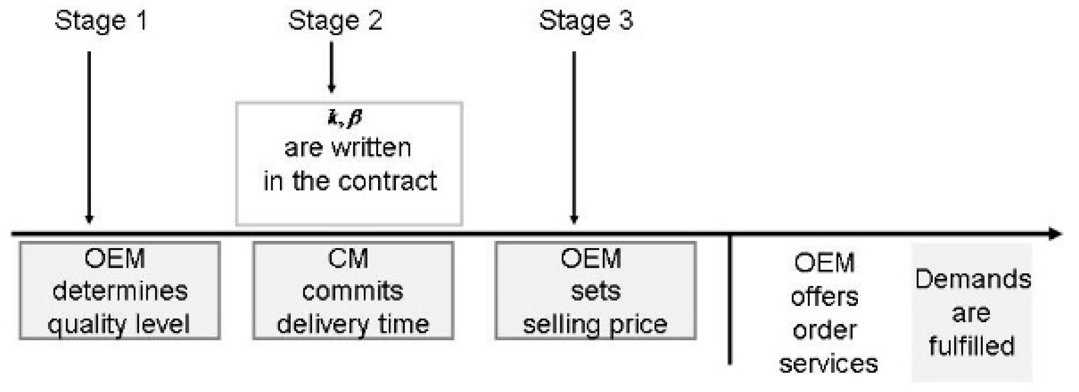
Specifically, we aim to study the optimal policies on quality and committed delivery time and identify the effects of system parameters in a build-to-order supply chain (BTO-SC), which consists of one contract manufacturer (CM) and one original equipment manufacturer (OEM). Under the quality–price–committed delivery time-sensitive demand, the CM decides on the committed delivery time of the supply chain product, and the OEM determines the quality level and the selling price of the supply chain product to maximize their respective profits. We first formulate the decisions of the CM and the OEM as a three-stage Stackelberg game, where the OEM is the leader. We then identify a Nash equilibrium solution for the decisions of the CM and the OEM. Finally, a sensitivity analysis is conducted, and some interesting results are found. For example, the OEM’s profit is non-monotonic in regard to the committed delivery time sensitivity of demand, and the CM’s profit is non-monotonic in terms of both the unit production subsidy paid by the OEM to the CM and the CM’s production capacity. Moreover, the optimal committed delivery time is non-monotonic regarding the unit production subsidy paid by the OEM to the CM.

We summarize the research contributions of our work (i.e., novelty of this research), as follows:

(1) Although some papers consider quality choice or committed delivery time, to the best of our knowledge, this study is the first integration of the two within a supply chain.

(2) Our results provide the OEM with insights into how to decide an optimal product quality and price, as well as the CM, in terms of how to decide on the optimal committed delivery time, in order to enhance the competitive advantages of BTO-SC. For example, the high-quality and fast-delivery product policy is worthwhile in a quality-sensitive or delivery time-sensitive market, which leads to a triple-win outcome among the CM, the OEM, and the customers.

(3) We prove the counterintuitive result that a high production capacity is not always advantageous for the supply chain product, even for the CM. In addition, a moderate production subsidy improves the quality level and delivery service.

The remainder of this paper is organized as follows. In the next section, we briefly review the relevant literature. We then describe the notation used in this paper and the assumptions made for the problem model in Section 3. We present the problem model and show several theoretical results in Section 4. Parametric sensitivity analysis is conducted in Section 5, and a conclusion is provided in Section 6. Proof of the main theoretical results is presented in the Appendix A section at the end.

2. Literature Review

Our work relates to three main streams of research: build-to-order supply chain management (BTO-SCM), supply chain delivery time decisions, and supply chain quality choices. We now briefly review the literature on the three topics.

2.1. Build-To-Order Supply Chain Management

As a way to improve the response to customers, BTO-SC combines the characteristics of a make-to-order strategy with a forecast-driven make-to-stock strategy [11]. BTO-SCM has received a great deal of attention in recent years due to the success of high-tech companies such as Dell, BMW, and Compaq [12,13]. A significant number of research papers have been written on BTO-SCM. Christensen et al. [14] examine the effects of BTO and show that a BTO strategy can positively affect market performance through its influence on the application of supply chain knowledge. Krajewski et al. [15] explore the reaction strategies that suppliers use to respond to short-term dynamics of schedule changes in BTO-SC. The above papers investigate the problems of BTO-SCM through empirical analysis or case studies. In response, researchers have started to explicitly address the problems of BTO-SCM through modeling [16]. Yimer and Demirli [11] formulate a two-phase mixed integer linear programming model for material procurement, component fabrication, product assembly, and distribution scheduling of a BTO-SC. Konstantaras et al. [17] develop a profit maximization model to jointly determine the optimal selling price, return policy and modularity level for BTO products, and obtain closed-form optimal solutions under certain conditions imposed on the model’s parameters. The authors of all of the above literature focus on the problems of scheduling the BTO-supply chain system or the pricing of BTO products. Mansouri et al. [18] identify the gap between the modeling and optimization techniques developed in the literature and highlight the decision support needed in practice. The customer is a very important asset for a BTO-SC; Tavakkoli-Moghaddam and Ebrahimi [19], therefore, focus on both the manufacturer’s profit and the customer’s utility simultaneously, where demand is dependent on quality and price.

Motivated by the example of Qualcomm cited in the Introduction, in addition to quality and price, we add committed delivery time to the influential factors of demand in the BTO-SC. Therefore, we extend the above-mentioned literature to analytically model the interplay between the OEM and the CM regarding quality choice, pricing and committed delivery time.

2.2. Supply Chain Delivery Time Decision

One of the several reasons why customers and investors are increasingly opting for Dell is its faster response time. Stalk [20] points out that time is the next source of competitive advantage. In competitive industries, fast delivery is critical to winning market share. Empirical evidence has shown that customers are willing to pay a higher price for a faster and more reliable service [21]. In general, fast delivery is associated with high capacity costs or penalty costs [22]. Hence, it is very important to commit to an appropriate delivery time for the product in a cost-effective way [8]. Boyaci and Ray [9] study a profit-maximizing firm selling two substitutable products in a price- and time-sensitive market. They develop a model that integrates pricing and delivery time decisions with capacity costs and show how the firm should adapt its differentiation strategy in response to a change in its operating dynamics. Celik and Maglaras [23] consider a profit-maximizing make-to-order manufacturer that offers multiple products to a market of price- and delay-sensitive users. The authors derive near-optimal dynamic pricing and lead-time quotations by using an approximating diffusion control problem and further illustrate the value of joint pricing and lead-time control policies. Unlike the assumption of risk-neutral decision makers in most of the existing literature, Li et al. [24] examine how the decision maker’s risk aversion affects the optimal price, committed delivery time, and overall utility. Furthermore, Bushuev et al. [25] investigate the effect of changes to the parameters of the delivery time distribution on the expected penalty costs for untimely delivery when a supplier uses an optimally positioned delivery window to minimize the expected costs of untimely delivery. Xu et al. [26] study the coordination of a supply chain with an online platform considering delivery time decisions. Hammami et al. [27] explore the delivery time quotation and pricing in a two-stage make-to-order supply chain facing time- and price-sensitive demand. Furthermore, the authors provide insights into the impact of market characteristics and capacities on the performance of a supply chain. Similarly, Hammami et al. [28] analytically characterize the interplay between local lead times, overall lead time, prices, and profits in decentralized supply chains.

It is worth mentioning that the above-mentioned literature pays little attention to the effect of the supply chain product quality on the demand and thus ignores the importance of quality choice for a BTO-SC. Our paper contributes to this theme by extending the research to investigate the integrated effects of pricing, delivery time decisions and quality choice.

2.3. Supply Chain Quality Choice

Product quality is increasingly valued by consumers, and thus the choice of supply chain quality is vital to a BTO-SC characterized by its personalization and customization. Balachandran and Rajan [29] analyze the relationship between the product quality and the cost of quality. Dogan et al. [30] propose a model to investigate the optimal quality improvement path for a company given that quality costs depend on both autonomous and induced types of learning experiences and a number of quality characteristics. Xu [10] studies a joint pricing and product quality decision problem in a distribution channel. Xie et al. [31] investigate the quality investment and price decision of a make-to-order supply chain with uncertain demand in international trade. Moreover, Chen et al. [32] highlight the importance of having a cooperative quality investment strategy and propose a simple proportional investment sharing schedule in the outsourcing of a supply chain. Ha et al. [2] study a supply chain with manufacturer encroachment in which product quality is endogenous and customers have heterogeneous preferences for quality. When quality is endogenous and the manufacturer has enough flexibility to adjust quality, the authors find that encroachment always negatively affects the retailer.

In recent years, supply chain quality choice is still the focus of many researchers. Fan et al. [33] investigate product quality choice in two-echelon supply chains under the post-sale liability of the upstream manufacturer. Their results show that post-sale product liability positively affects the wholesale price and quality level, but not supply chain members’ profitability. Additionally, the authors extend their research to consider liability cost sharing amongst supply chain members [34]. Zhou et al. [35] explore optimal product quality and service quality with reference to their effect in dual-channel supply chains and propose an effective service cost-sharing coordinating contract. With the wide acceptance of sustainable development, researchers are increasingly paying attention to supply chain quality choice in the remanufacturing context. For example, Zhao et al. [36] examine how an OEM utilizes product quality to compete with a third-party remanufacturer in the presence of a trade-in program. The authors find that the OEM almost always increases product quality and makes more profit in the trade-in context. Similarly, He et al. [37] consider the economic and environmental implications of quality choice under remanufacturing outsourcing and find that the OEM is more likely to choose a lower quality for new products when outsourcing remanufacturing to CMs. Moreover, Zou et al. [38] examine how downstream retailers’ remanufacturing operations affect the OEM’s quality choice of new products. The above literature addresses supply chain quality choice and pricing in different contexts, but does not pay any attention to the fact that customers are increasingly sensitive to supply chain product delivery time. In contrast, we contribute to this research theme by linking the quality choice literature with the delivery service literature.

In summary, the above-mentioned research only considers either the delivery time decisions or quality choice in a BTO-SC. However, this research extends the understanding of these three themes of research by integrating delivery time decisions with quality choice in a BTO-SC. This approach allows us to explore how to trade off the decisions on delivery time and product quality for a BTO-SC meeting quality–price–committed delivery time-sensitive demand, and thus to reveal the optimal equilibrium decisions on delivery time and product quality.

3. Notation and Assumptions

Before we model the decisions of the CM and the OEM, we define our notations and make related assumptions.

3.1. Notation

$Q_m$: quality level of product chosen by the OEM.

$P_m$: unit selling price of product set by the OEM.

$T_s$: CM committed delivery time of product.

$T_a$: actual delivery time of the product.

$a$: potential market size for the product.

$b$: selling price sensitivity of demand.

$c$: quality sensitivity of demand.

$d$: committed delivery time sensitivity of demand.

$\lambda$: mean arrival rate or expected demand per unit time.

$\xi$: technical parameter indicating the investment level needed for quality improvement.

$\alpha$: marginal cost related to the quality.

$k$: unit production subsidy related to the quality paid by the OEM to the CM.

$\mu$: CM’s capacity per unit time.

$\beta$: unit compensation fees (penalty costs) paid by the CM to the customer.

${\prod }_m$: OEM’s expected profit per unit time.

${\prod }_s$: CM’s expected profit per unit time.

3.2. Assumptions

We assume that customers arrive at the BTO-SC system to place an order according to a Poisson process. The mean arrival rate depends linearly on the selling price, the product quality level, and the committed delivery time. We also assume that the mean arrival rate decreases in accordance with the selling price and in the committed delivery time, and increases in accordance with the product quality level [24,32,39], i.e.,

$$\lambda \left(P_m,Q_m,T_s\right)=a-b{P}_m+c{Q}_m-d{T}_s$$

Similarly to Boyaci and Ray [9], we assume that both the OEM and the CM consider maximizing their expected profits per unit time. Clearly, the expected demand per unit time is equal to the mean arrival rate under our assumption that each arriving customer would buy only one product.

The OEM decides the product quality level and takes on the fixed expenses of quality investment $\frac{1}{2}\xi Q_m^2$, which involves investment in design, device, and process [40,41,42].

The CM organizes the production and takes on the variable expenses of quality investment in each product $\alpha Q_m$, which involves investment in raw materials and skilled laborers. For simplicity, we only consider the variable costs related to the quality. Following the industry standard, the OEM pays a subsidy $k{Q}_m$ to the CM for producing each product [32]. Here, the assumption of $k>\alpha$ is needed to ensure that the CM makes positive production profits.

For a BTO-SC system, we further assume that the CM’s capacity per unit time is much greater than the mean arrival rate (i.e., $\mu \gg \lambda$). This means that the actual delivery time of a product is approximately equal to its production time. As shown in the literature [43], the production time distribution is well approximated by the exponential distribution. Therefore, we reasonably assume that the actual delivery time $T_a$ follows the exponential distribution with the parameter $\mu$.

A certain compensation fee amount is paid by the CM to the customer when a random customer’s actual delivery time is later than the committed delivery time [44]. In this paper, we refer to the compensation fees as the penalty costs incurred by the CM. Under our exponential actual delivery time assumption, the mean compensation fees for each customer are:

$$\beta {{\displaystyle \int }}_{T_s}^{\infty }\left(t-T_s\right)\mu e^{-\mu t}dt=\frac{\beta }{\mu }{e}^{-\mu T_s}$$

In this paper, all the variables and parameters are assumed to be positive. Furthermore, we assume that both the OEM and the CM are risk neutral, and all the information is symmetrical between them.

Remark 1.

We consider both the unit production subsidy$k$and the unit compensation fees$\beta$as exogenous parameters, not decision variables, which is reasonable for a well-established industry. In fact,$k$and$\beta$are able to be set through referring to the industry standard or negotiation between the CM and the OEM.

4. Model and Analysis

4.1. The Model

In an outsourcing mode, one can expect that the OEM always has full power over the product quality choice [32,40]. Therefore, in our scenario, the OEM first makes the quality decision and takes on its fixed investment expenses, and then outsources the production to the CM by paying a subsidy. Since customers are sensitive to the delivery time of a product, the committed delivery time in BTO-SC influences the demand (i.e., the quantity of production) and thus the amount of subsidy received by the CM. The CM then commits to the delivery time of a product and takes on the compensation fees paid to customers for a delayed delivery service [28]. Meanwhile, a contract is drawn up between the CM and the OEM, involving the production subsidy, the committed delivery time and the compensation fees. The OEM then sets the selling price for the supply chain product and offers order services to customers. When the order arrives at the BTO-SC system, the OEM notifies the CM to organize the production immediately, and the completed product is delivered directly to the customer by the CM. The above decision sequence is basically in line with the Qualcomm example cited in the introduction.

To describe the decision structure between the CM and the OEM, we present a three-stage game events sequence, as shown in Figure 1.

Under our relevant assumptions, the three-stage game above can be formulated as follows:

$$\underset{Q_m}{max}{\prod }_m\left(P_m,Q_m\right)=\left(P_m-k{Q}_m\right)\left(a-b{P}_m+c{Q}_m-d{T}_s\right)-\frac{\xi Q_m^2}{2}.$$

(1)

$$\underset{T_s}{max}{\prod }_s\left(T_s\right)=(k{Q}_m-\alpha Q_m-\frac{\beta }{\mu }{e}^{-\mu T_s})\left(a-b{P}_m+c{Q}_m-d{T}_s\right).$$

(2)

$$\underset{P_m}{max}{\prod }_m\left(P_m,Q_m\right)=\left(P_m-k{Q}_m\right)\left(a-b{P}_m+c{Q}_m-dT\right)-\frac{\xi Q_m^2}{2}.$$

(3)

4.2. The Model Analysis

We now solve this dynamic game by using backward induction.

4.2.1. Stage 3: OEM’s Selling Price Decision

We analyze the OEM’s selling price decision conditional on the CM’s committed delivery time and its own preceding quality level.

Taking the first-order derivative and the second-order derivative of ${\prod }_m\left(P_m,Q_m\right)$ with respect to $P_m$ in (3), we have

$$\frac{\partial {\prod }_m\left(P_m,Q_m\right)}{\partial P_m}=-2b{P}_m+a+\left(kb+c\right)Q_m-d{T}_s,\frac{{\partial }^2{\prod }_m\left(P_m,Q_m\right)}{\partial P_m^2}=-2b<0.$$

Clearly, ${\prod }_m\left(P_m,Q_m\right)$ is strictly concave in $P_m$ conditional on $T_s$ and $Q_m$. Let $\frac{\partial {\prod }_m\left(P_m,Q_m\right)}{\partial P_m}=0$, and thus we obtain the best response function of the selling price:

$$P_m\left(T_s,Q_m\right)=\frac{a+\left(kb+c\right)Q_m-d{T}_s}{2b}$$

(4)

Proposition 1.

$P_m\left(T_s,Q_m\right)$increases with$Q_m$and decreases with$T_s$.

Proof of Proposition 1.

Proposition 1 is direct from (4). □

Proposition 1 shows that the higher the quality level chosen by the OEM or the sooner the CM commits to the delivery time, the higher the selling price set by the OEM as a response.

Substituting (4) into $\lambda \left(P_m,Q_m,T_s\right)$, we have

$$\lambda \left(P_m\left(T_s,Q_m\right),Q_m,T_s\right)=\frac{1}{2}\left(a+\left(c-kb\right)Q_m-d{T}_s\right).$$

(5)

4.2.2. Stage 2: CM’s Committed Delivery Time Decision

We investigate the CM’s decision regarding committed delivery time conditional on the OEM’s quality level and in anticipation of the OEM’s selling price in Stage 3.

Substituting (4) into (2), we have

$${\prod }_s\left(T_s\right)=\frac{1}{2}(\left(k-\alpha \right)Q_m-\frac{\beta }{\mu }{e}^{-\mu T_s})\left(a+\left(c-kb\right)Q_m-d{T}_s\right).$$

(6)

Taking the first-order derivative and the second-order derivative of ${\prod }_s\left(T_s\right)$ with respect to $T_s$ in (6), we have

$$\frac{d{\prod }_s\left(T_s\right)}{d{T}_s}=-\frac{1}{2}\left(k-\alpha \right)d{Q}_m+\frac{1}{2}\beta (a+\frac{d}{\mu }+\left(c-kb\right)Q_m-d{T}_s)e^{-\mu T_s},$$

(7)

$$\frac{d^2{\prod }_s\left(T_s\right)}{d{T}_s^2}=-\frac{\beta \mu }{2}(a+\frac{2d}{\mu }+\left(c-kb\right)Q_m-d{T}_s)e^{-\mu T_s}.$$

(8)

Lemma 1.

$\lambda$is non-negative if and only If$0<T_s\le \frac{a+\left(c-kb\right)Q_m}{d}.$

Proof of Lemma 1.

Lemma 1 is direct from (5). □

Lemma 1 shows that there is an upper-bounded value of the committed delivery time for guaranteeing a non-negative mean arrival rate conditional on the OEM’s quality level.

Theorem 1

${\prod }_s\left(T_s\right)$is strictly concave in$T_s\in (0,\frac{a+\left(c-kb\right)Q_m}{d}]$for any given$Q_m>0$.

Proof of Theorem 1.

From (8), it is easy to see that $\frac{d^2{\prod }_s\left(T_s\right)}{d{T}_s^2}<0$ when $T_s\in (0,\frac{a+\left(c-kb\right)Q_m}{d}].$ Therefore, ${\prod }_s\left(T_s\right)$ is strictly concave in $T_s\in (0,\frac{a+\left(c-kb\right)Q_m}{d}]$ for any given $Q_m>0$ This proves this theorem. □

Lemma 2.

If$\beta \left(c-kb\right)\le \left(k-\alpha \right)d$, then the equation$\frac{d{\prod }_s\left(T_s\right)}{d{T}_s}=0$determines a unique implicit function$T_s\left(Q_m\right)$in the area of$T_s\times Q_m$, where$T_s\in \left(0,\frac{a+\left(c-kb\right)Q_m}{d}\right]$and$Q_m\in [\frac{\beta }{\mu \left(k-\alpha \right)}, \frac{\beta \left(a+\frac{d}{\mu }\right)}{\left(k-\alpha \right)d-\beta \left(c-kb\right)}]$.

Proof of Lemma 2.

See Appendix A. □

Remark 2.

The parametric condition$\beta \left(c-kb\right)\le \left(k-\alpha \right)d$is easy to satisfy for the relatively high unit production subsidy compared to the unit penalty costs. The above parametric condition is assumed to hold in the following theoretic discussion.

Corollary 1.

The best response function of committed delivery time is$T_s\left(Q_m\right)$for any given quality $Q_m\in [\frac{\beta }{\mu \left(k-\alpha \right)}, \frac{\beta \left(a+\frac{d}{\mu }\right)}{\left(k-\alpha \right)d-\beta \left(c-kb\right)}]$.

Proof of Corollary 1.

This corollary is from Theorem 1 and Lemma 2. □

Proposition 2.

$T_s\left(Q_m\right)$decreases with$Q_m$.

Proof of Proposition 2.

See Appendix A. □

Proposition 2 shows that the higher the quality level chosen by the OEM, the sooner the CM commits to the delivery time in response. The CM is more likely to make a positive unit profit at a higher quality level. Moreover, the sooner the committed delivery time is, the higher the demand is, and thus a higher the number of products need to be produced. Therefore, the CM has an incentive to commit to a relatively short delivery time so as to make more profits when the quality level is high, given that the unit production subsidy is relatively high compared to the unit penalty costs.

Substituting $T_s\left(Q_m\right)$ into (4), we have

$$P_m\left(T_s\left(Q_m\right),Q_m\right)=\frac{a+\left(kb+c\right)Q_m-d{T}_s\left(Q_m\right)}{2b}.$$

(9)

For convenience of writing, we denote $P_m\left(Q_m\right):=P_m\left(T_s\left(Q_m\right),Q_m\right)$.

Proposition 3.

$P_m\left(Q_m\right)$increases with$Q_m$.

Proof of Proposition 3.

This proposition is from (9) and Proposition 2. □

Proposition 3 shows that the higher the quality level chosen by the OEM, the higher the selling price that is set. Therefore, the selling price is finally determined by the quality level of the product in the BTO-SC.

Substituting $T_s\left(Q_m\right)$ into (5), we have

$$\lambda \left(P_m\left(T_s\left(Q_m\right),Q_m\right),Q_m,T_s\left(Q_m\right)\right)=\frac{1}{2}\left(a+\left(c-kb\right)Q_m-d{T}_s\left(Q_m\right)\right).$$

(10)

For convenience of writing, we denote $\lambda \left(Q_m\right):=\lambda \left(P_m\left(T_s\left(Q_m\right),Q_m\right),Q_m,T_s\left(Q_m\right)\right)$.

Proposition 4.

If$c-kb\ge 0$, then $\lambda \left(Q_m\right)$increases with$Q_m$.

Proof of Proposition 4.

This proposition is from (10) and Proposition 2. □

Proposition 4 shows that when customers are more sensitive to the quality than to the selling price of a product, a higher quality level is chosen by the OEM, and the mean arrival rate will be higher.

Remark 3.

From Propositions 3–4, we can see that the OEM’s sales revenue increases at the quality level. However, both the amount of production subsidy paid to the CM and the fixed expenses of quality investment taken by the OEM also increase as the quality level increases. Hence, the OEM needs to determine the optimal quality level to maximize its profit.

4.2.3. Stage 1: OEM’s Quality Choice

We examine the OEM’s quality choice in anticipation of the CM’s committed delivery time in Stage 2 and its selling price in Stage 3.

Substituting $P_m\left(Q_m\right)$ and $T_s\left(Q_m\right)$ into (1), we have

$${\prod }_m\left(P_m\left(Q_m\right),Q_m\right)=\frac{{(a+\left(c-kb\right)Q_m-d{T}_s\left(Q_m\right))}^2}{4b}-\frac{\xi Q_m^2}{2}.$$

(11)

For convenience, we denote ${\prod }_m\left(Q_m\right):={\prod }_m\left(P_m\left(Q_m\right),Q_m\right)$ and $T_s^{\prime }\left(Q_m\right):=\frac{d{T}_s\left(Q_m\right)}{d{Q}_m}$.

Taking the first-order derivative of ${\prod }_m\left(Q_m\right)$ with respect to $Q_m$, we have

$$\frac{d{\prod }_m\left(Q_m\right)}{d{Q}_m}=\frac{\left(a+\left(c-kb\right)Q_m-d{T}_s\left(Q_m\right)\right)\left(c-kb-d{T}_s^{\prime }\left(Q_m\right)\right)}{2b}-\xi Q_m,$$

(12)

where

$${T_s}^{\prime }\left(Q_m\right)=\frac{\beta \left(c-kb\right)-\left(k-\alpha \right)d{e}^{\mu T_s\left(Q_m\right)}}{\beta \mu (\frac{2d}{\mu }+a+\left(c-kb\right)Q_m-d{T}_s\left(Q_m\right))},$$

(13)

and $T_s\left(Q_m\right)$ satisfies the equation

$$\beta (a+\frac{d}{\mu }+\left(c-kb\right)Q_m-d{T}_s\left(Q_m\right))-\left(k-\alpha \right)d{Q}_m{e}^{\mu T_s\left(Q_m\right)}=0.$$

(14)

Lemma 3.

$T_s\left(Q_m\right)<\frac{a+\frac{\beta \left(c-kb\right)}{\left(\mu \left(k-\alpha \right)\right)}}{2d}$for$Q_m\in [\frac{\beta }{\mu \left(k-\alpha \right)}, \frac{\beta \left(a+\frac{d}{\mu }\right)}{\left(k-\alpha \right)d-\beta \left(c-kb\right)}]$

Proof Lemma 3.

Substituting $Q_m=\frac{\beta }{\mu \left(k-\alpha \right)}$ into (14) and organizing the left-hand side of the equation, we have

$$\beta (a+\frac{\beta \left(c-kb\right)}{\mu \left(k-\alpha \right)})-\frac{\beta d}{\mu }(e^{\mu T_s(\frac{\beta }{\mu \left(k-\alpha \right)})}-1+\mu T_s(\frac{\beta }{\mu \left(k-\alpha \right)}))=0.$$

(15)

Since $e^x-1>x$ for $x>0$, from (15), we have $a+\frac{\beta \left(c-kb\right)}{\mu \left(k-\alpha \right)}-2d{T}_s(\frac{\beta }{\mu \left(k-\alpha \right)})>0$. This means $T_s(\frac{\beta }{\mu \left(k-\alpha \right)})<\frac{a+\frac{\beta \left(c-kb\right)}{(\mu \left(k-\alpha \right)}}{2d}$. Moreover, $T_s\left(Q_m\right)\le T_s(\frac{\beta }{\mu \left(k-\alpha \right)})$ when $Q_m\ge \frac{\beta }{\mu \left(k-\alpha \right)}$ from Proposition 2. Therefore, this lemma holds. □

Theorem 2.

${\prod }_m\left(Q_m\right)$contains a maximizer,$Q_m^{*},$, which satisfies the first-order condition

$$\frac{\left(a+\left(c-kb\right)Q_m-d{T}_s\left(Q_m\right)\right)\left(c-kb-d{T}_s^{\prime }\left(Q_m\right)\right)}{2b}-\xi Q_m=0.$$

Proof of Theorem 2.

See Appendix A. □

Theorem 2 shows that the OEM can decide on the optimal quality level to maximize its profit in the BTO-SC.

We denote $T_s^{*}:=T_s\left(Q_m^{*}\right)$, $P_m^{*}:=P_m\left(Q_m^{*}\right).$

Proposition 5.

$\left(Q_m^{*},T_s^{*},P_m^{*}\right)$is a Nash equilibrium solution of the decisions of the CM and the OEM in BTO-SC.

Proof of Proposition 5.

As the leader of the three-stage game, the OEM first chooses the quality level $Q_m^{*}$ to maximize its profit from Theorem 2. As a response, the CM then commits to the delivery time $T_s^{*}$ conditional on $Q_m^{*}$ from Corollary 1. As a response, the OEM finally sets the selling price $P_m^{*}$ conditional on $Q_m^{*}$ and $T_s^{*}$ from (9). Therefore, $\left(Q_m^{*},T_s^{*},P_m^{*}\right)$ is a Nash equilibrium of the three-stage game. □

Denote the optimal OEM’s and CM’s profits as ${\prod }_m^{*}:={\prod }_m\left(Q_m^{*}\right)$ and ${\prod }_s^{*}:={\prod }_s\left(T_s^{*}\right)$, respectively.

5. Sensitivity Analysis

In this section, we conduct a sensitivity analysis to explore the influences of several main system parameters on the optimal supply chain members’ decisions and their profits.

5.1. Description

According to our theoretic research results, the existence of equilibrium points can be guaranteed if parameters here simultaneously satisfy the following conditions:

$$k>\alpha ,\beta \left(c-kb\right)\le \left(k-\alpha \right)d,\lambda <<\mu ,\frac{\left(a\mu +\omega \right)\left(\omega +d\right)\left(a\mu +\omega +d\right)}{\mu \left(a\mu +\omega +2d\right)}-\frac{2b\xi {\omega }^2}{\mu {(c-kb)}^2}<0,\frac{\left(a\mu +\gamma \right)\left(\gamma +d\right)\left(a\mu +\gamma +2d\right)}{2\mu \left(a\mu +\gamma +4d\right)}-\frac{2b\xi {\gamma }^2}{\mu {(c-kb)}^2}>0,\gamma =\frac{\beta \left(c-kb\right)}{k-\alpha },\omega =\frac{\beta \left(a\mu +d\right)\left(c-kb\right)}{\left(k-\alpha \right)d-\beta \left(c-kb\right)}.$$

Let $a=30$, $b=1$, $c=5$, $d=2$, $k=4$, $\alpha =2$, $\beta =1$, $\mu =50$, $\xi =6$. For the above value of parameters, we can obtain a unique Nash equilibrium solution $\left(Q_m^{*},T_s^{*},P_m^{*}\right)$ by solving the system of equations $\frac{d{\prod }_m\left(Q_m\right)}{d{Q}_m}=0$ and $\frac{d{\prod }_s\left(T_s\right)}{d{T}_s}=0$. As shown in Figure 2, there is a unique Nash equilibrium point $\left(Q_m^{*},T_s^{*}\right)$. Therefore, we take them as a set of basic value of parameters. However, there may be multiple Nash equilibrium points as the value of some parameters is changed. For the situation where there are multiple Nash equilibrium points, we only consider the equilibrium point at which the leader OEM’s profit is maximized.

In addition, our search for the equilibrium points is limited to the area $T_s\times Q_m$ so as to improve the computational efficiency, where

$$T_s\in \left(0,\frac{a+\left(c-kb\right)Q_m}{d}\right]\mathrm{and}{Q}_m\in [\frac{\beta }{\mu \left(k-\alpha \right)}, \frac{\beta \left(a+\frac{d}{\mu }\right)}{\left(k-\alpha \right)d-\beta \left(c-kb\right)}].$$

5.2. Sensitivity to Parameter $b$

To study the sensitivity of the optimal decisions and profits to parameter $b$, we vary the value of $b$ and fix a basic value for the other parameters.

As shown in Figure 3, the selling price and the quality level set by the OEM decrease first sharply and then more slowly, while the delivery time set by the CM slowly increases with the selling price sensitivity of demand. The explanation for this is that the OEM’s first response is to cut the selling price to promote demand when customers become more sensitive to the selling price of a product. As a result, the OEM correspondingly lowers the quality level considering the cost of quality investment and the low marginal sales revenue. The CM obtains the low unit production subsidy for the low-quality level and thus has no incentive to promote the demand by shortening the delivery time considering the penalty costs.

Although the selling price falls, the low-quality level and the long delivery time of the product still lead to a corresponding reduction in the demand from our computational results. Therefore, both the OEM’s profit and the CM’s profit decrease sharply initially and then more slowly as the selling price sensitivity of demand increases, as shown in Figure 4. This leads to the observation that a market of price-sensitive customers does not improve the quality and delivery service, or the profits of supply chain members. Furthermore, when the selling price sensitivity of demand exceeds a certain threshold value, supply chain members may withdraw from the market since the CM is unprofitable and the OEM’s profit is also very low.

5.3. Sensitivity to Parameter $c$

In this section, we fix a basic value for the other parameters and vary the value of $c$ to examine its effect on optimal decisions and profits.

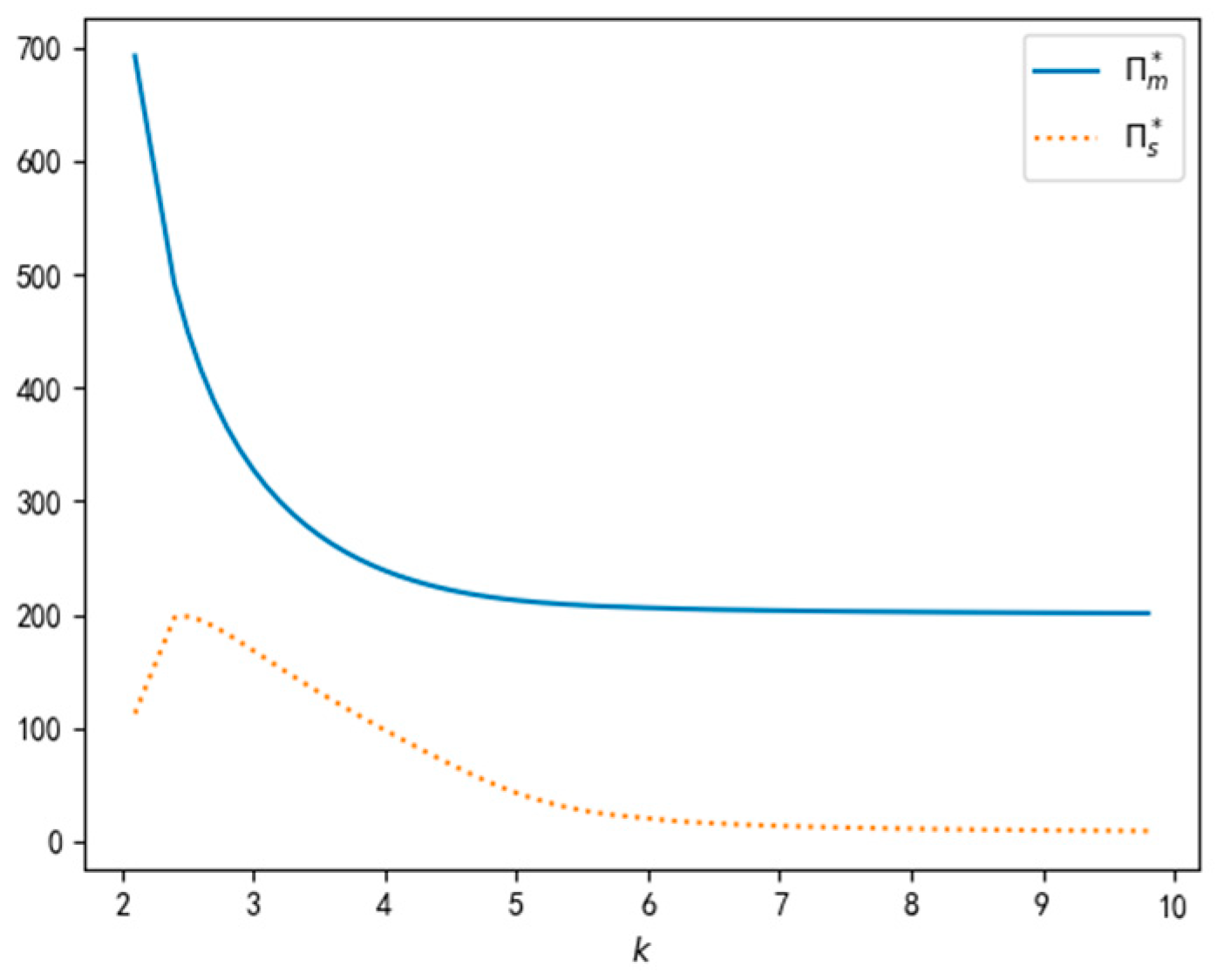
Intuitively, the selling price and the quality level set by the OEM increase with the quality sensitivity of demand. Interestingly, the delivery time set by the CM decreases with the quality sensitivity of demand, as shown in Figure 5. The reason for this is that the OEM tends to improve the quality and reasonably raise the selling price when customers value the quality of a product. In view of the high unit production subsidy related to the high quality level, the CM has an incentive to commit to a short delivery time so as to promote the demand and thus obtain more production subsidies. This implies that the high customer awareness of quality benefits the interactions between supply chain members. Therefore, as shown in Figure 6, the supply chain members’ profits increase as the demand increases. More interestingly, the follower CM’s profit even exceeds the leader OEM’s profit if the quality sensitivity of demand is high enough.

In summary, a market of quality-sensitive customers helps to improve the quality of a product and the delivery service and increase supply chain members’ profits, hence enabling a triple-win outcome.

5.4. Sensitivity to Parameter $d$

To explore the impact of parameter $d$ on the optimal decisions and profits, we vary the value of $d$ and fix a basic value for the other parameters.

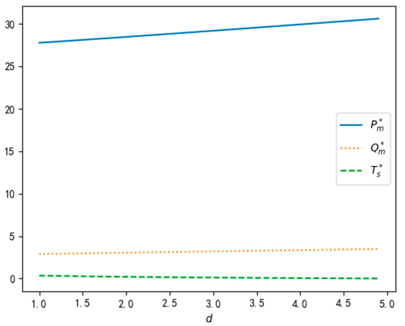
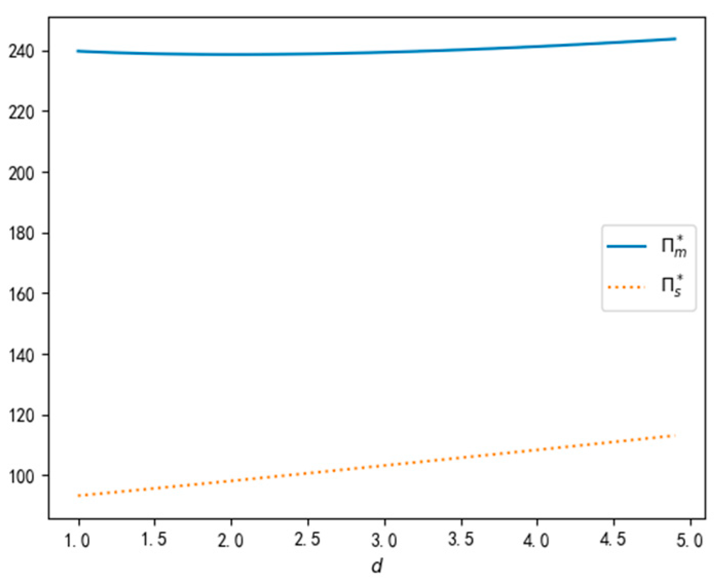
Compared with parameter $c$, parameter $d$ has the same trend of impact on the optimal decisions, but the sensitivities of the selling price and the quality level of it are much smaller, as shown in Figure 7. The explanation for this is that the CM has an incentive to commit to a short delivery time to promote the demand when customers value the delivery service of a product. However, the CM’s effort level depends on the quality level chosen by the OEM since the production subsidy is related to the quality. Predicting the CM’s response and considering the costs of quality investment, the OEM moderately increases the quality level to encourage the CM to shorten the delivery time. Conditional on the small increase in the quality by the OEM, the CM also slightly shortens the delivery time considering the penalty costs. Correspondingly, the OEM gradually increases the selling price. From our computational results, the demand first decreases and then increases slowly as the committed delivery time sensitivity of demand increases. This implies that the selling price initially has a more dominant influence on the demand than the quality level and the delivery time. As a result, the OEM’s profit has the same variation pattern as the demand when the committed delivery time sensitivity of demand varies, as shown in Figure 8, whereas intuitively, the CM’s profit increases with the committed delivery time sensitivity of demand due to the increased quality level.

In summary, a market of high delivery time-sensitive customers has a small positive impact on improving the quality and the delivery service and increasing supply chain members’ profits. A medium delivery time sensitivity of demand is not beneficial to the leader OEM. Counterintuitively, customers can enjoy the high-quality product alongside a fast delivery service when they become more sensitive to the committed delivery time.

5.5. Sensitivity to Parameter $k$

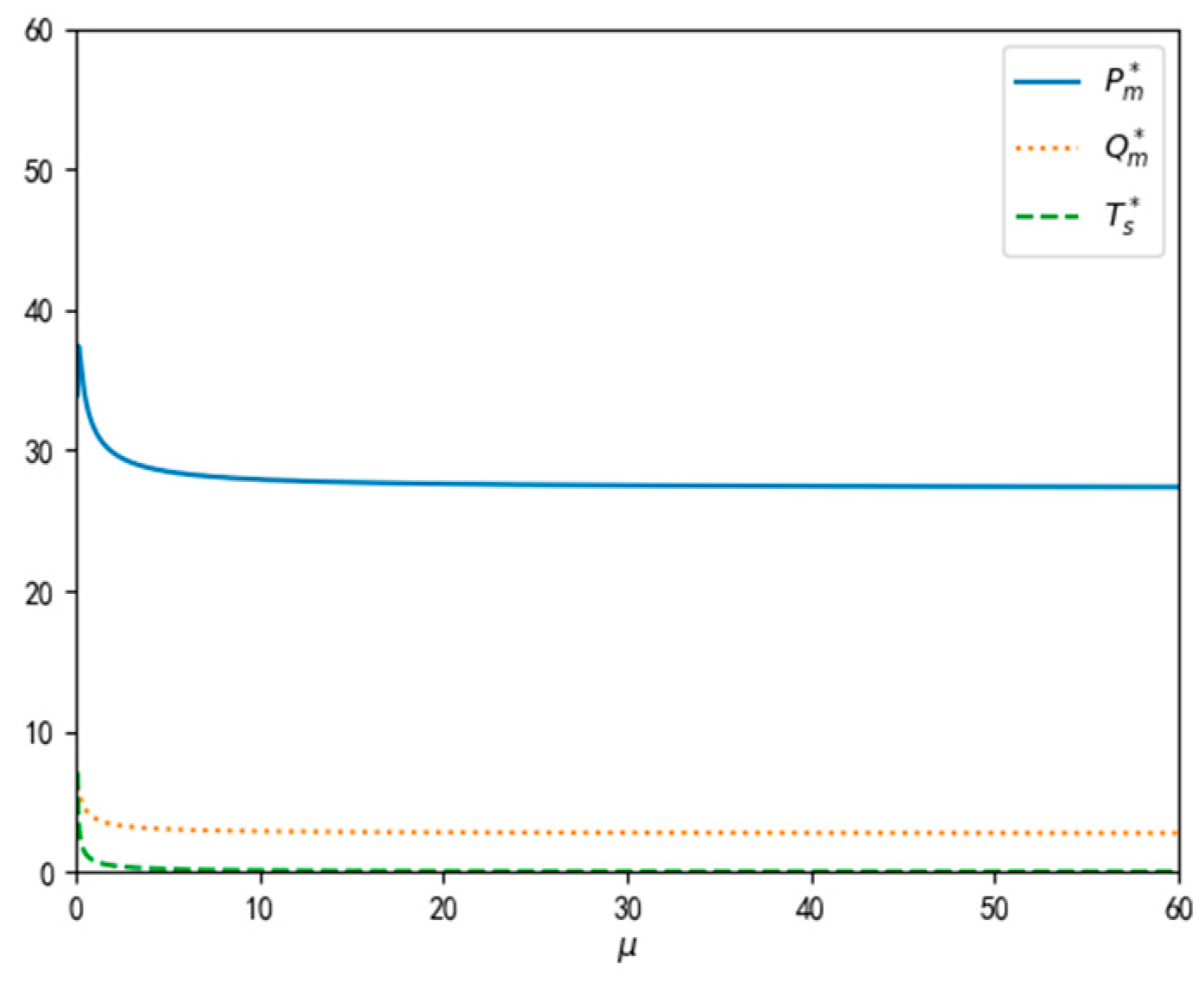
In this section, we study the impact of the unit production subsidy related to the quality on the optimal decisions and profits by varying the value of parameter $k$.

As shown in Figure 9, the selling price and the quality level set by the OEM decrease, while the delivery time set by the CM first decreases and then increases as the unit production subsidy related to the quality increases. The OEM’s profit decreases intuitively, while the CM’s profit first increases and then decreases as the value of parameter $k$ increases, as shown in Figure 10. The explanation for this is that, when the value of parameter $k$ increases, the OEM lowers the quality level to reduce the transfer payment and correspondingly cuts the selling price to promote the demand. The CM initially has an incentive to shorten the delivery time as the unit production subsidy increases. However, such an incentive gradually becomes weak as the quality level decreases, and then the CM prolongs the delivery time considering the penalty costs. From our computational results, the demand continues to decrease in the equilibrium, which leads to a decrease in the OEM’s profit. Interestingly, the increase in the unit production subsidy is harmful to the CM after it exceeds the threshold value.

In summary, too high a unit production subsidy does not improve the quality and the delivery service, and even damages supply chain members’ profits. If $k$ is determined through negotiation between the CM and the OEM, it is good for the CM to claim a moderate unit production subsidy instead of asking for excessively high processing compensation.

5.6. Sensitivity to Parameter $\mu$

To examine the impact of the CM’s capacity on the optimal decisions and profits, we vary the value of parameter $\mu$ and fix a basic value for the other parameters.

Both the quality level and the selling price set by the OEM decrease slowly, while the delivery time set by the CM is almost constant, and the OEM’s profit increases with the CM’s capacity, as shown in Figure 11 and Figure 12, whereas the impact of the CM’s capacity on its own profit is non-monotonic; that is, the CM’s profit first increases temporally and then decreases continuously as the CM’s capacity increases, as shown in Figure 12. The reason for this is that, when the CM’s capacity increases, the CM is willing to commit to a short delivery time due to the decrease in the expected penalty costs. Predicting this, the OEM chooses to lower the quality level so as to save the quality investment costs and accordingly reduce the selling price to promote the demand. As the quality level continuously decreases, the demand decreases from our computational results. As a result, the OEM’s profit increases slowly due to the decrease in quality investment costs, although the demand decreases slowly. The initial increase in the CM’s profit results from the decrease in expected penalty costs. However, the production subsidy decreases as the quality level continuously decreases, and thus the demand decreases. This results in the change pattern of the CM’s profit shown in Figure 12 when its capacity changes. Interestingly, the improvement in the CM’s capacity always benefits the leader OEM, while the CM’s over-capacity can even harm it.

In summary, a high production capacity helps to lower the selling price but can harm the quality, and a medium production capacity increases supply chain members’ profits. Surprisingly, the delivery time in the equilibrium is not sensitive to the CM’s production capacity.

6. Conclusions

This paper studies the optimal quality choice and committed delivery time in a build-to-order supply chain, which consists of one contract manufacturer and one original equipment manufacturer. Under our assumptions, we provide closed-form or easily computed solutions regarding the decisions of the contract manufacturer and the original equipment manufacturer. We prove the existence of an equilibrium solution for their decisions. A detailed sensitivity analysis identifies how various system parameters affect the optimal supply chain members’ decisions and profits. This analysis enables us to identify several valuable insights into build-to-order supply chains.

(1) From Proposition 2, Proposition 4 and Proposition 5, the high-quality and fast-delivery product policy is worthwhile in a quality-sensitive or delivery time-sensitive market, which leads to a triple-win outcome among the contract manufacturer, the original equipment manufacturer, and the customers. This mirrors Tesla’s product policy cited in the Introduction.

(2) A moderate production subsidy can improve the quality and the delivery service (Figure 9), as well as supply chain members’ profits (Figure 10). Hence, the contract manufacturer’s rational compromises in processing compensation help not only the original equipment manufacturer but also itself. This mirrors Qualcomm’s outsourcing production policy cited in the Introduction.

(3) A high production capacity does not always mean an advantage for the supply chain product, even for the contract manufacturer (Figure 12). A medium production capacity is desirable in a quality-sensitive market since over-capacity hurts the quality of the product (Figure 11).

(4) Supply chain members typically benefit from their cooperation partners improving the quality level or the delivery service. In a highly quality-sensitive market, the follower’s profit may even exceed the leader’s through the latter’s efforts in quality improvement. In a highly delivery time-sensitive market, as a leader, the original equipment manufacturer is encouraged to select a contract manufacturer with a relatively high production capacity [27].

(5) Considering the opportunity costs of quality investment, supply chain members are encouraged to drop unprofitable businesses in a market of highly selling price-sensitive customers. This mirrors Johnson & Johnson’s drug-coated stent market policy [45].

Our work suggests several interesting directions for further research. First, a similar problem can be studied under the different random demand, for example, the renewal process with a nonlinear mean arrival rate. Second, here, we assume that supply chain members are risk neutral. It should be possible to generalize our results to consider supply chain members with different risk attitudes. Third, it would be interesting to study a horizontal competitive environment with multiple contract suppliers of different production capacities. Finally, a game events sequence different from those considered here can be explored. In conclusion, we hope that our work will encourage the further investigation of the intriguing and important topic of product and service operation management in supply chains.

References

1. Model3 Tesla China-Tesla. Available online: https://www.tesla.cn/model3 (accessed on 1 May 2019).
2. Ha, A.; Long, X.; Nasiry, J. Quality in supply chain encroachment. Manuf. Serv. Oper. Manag. 2016, 18, 280–298. [Google Scholar] [CrossRef]
3. So Long After the Explosion, Why Is Samsung Still Losing Ground in China? Available online: http://news.ikanchai.com/2017/0924/160592.shtml (accessed on 1 May 2019).
4. Snapdragon 8GEN1 Becomes “Low Price Goods”, 120W Flash Charge +1920Hz Dimming, Down to RMB 2169! Available online: https://baijiahao.baidu.com/s?id=1739579669939566618&wfr=spider&for=pc (accessed on 28 July 2022).
5. What is the Reason Why Snapdragon 8GEN1 Overheating Is Still Serious? Available online: https://www.zhihu.com/question/510499326/answer/2528403143 (accessed on 14 June 2022).
6. Qualcomm’s Half-Year Deep Reform, Snapdragon 8+ Gen1 Efficacy Performance Is Perfect. Available online: https://baijiahao.baidu.com/s?id=1742120157475461797&wfr=spider&for=pc (accessed on 25 August 2022).
7. Modak, N.M.; Kelle, P. Managing a dual-channel supply chain under price and delivery-time dependent stochastic demand. Eur. J. Oper. Res. 2019, 272, 147–161. [Google Scholar] [CrossRef]
8. Salari, N.; Liu, S.; Shen, Z.-J.M. Real-time delivery time forecasting and promising in online retailing: When will your package arrive? Manuf. Serv. Oper. Manag. 2022, 24, 1261–1885. [Google Scholar] [CrossRef]
9. Boyaci, T.; Ray, S. Product differentiation and capacity costs interaction in time and price sensitive markets. Manuf. Serv. Oper. Manag. 2003, 5, 18–36. [Google Scholar] [CrossRef]
10. Xu, X. Optimal price and product quality level decisions in a distribution channel. Manag. Sci. 2009, 55, 1347–1352. [Google Scholar] [CrossRef]
11. Yimer, A.D.; Demirli, K. A genetic approach to two-phase optimization of dynamic supply chain scheduling. Comput. Ind. Eng. 2010, 58, 411–422. [Google Scholar] [CrossRef]
12. Lakshmi, S. Make to order strategy at Dell Corporation: A case study. Aweshkar 2018, 25, 21–27. [Google Scholar]
13. Parvez, M.; Ullah, N.; Sabuj, M.A.; Islam, S. Profit maximization of DELL Inc. through Build-to-Order supply chain for laptop manufacturing. Am. J. Ind. Bus. Manag. 2018, 8, 1657–1671. [Google Scholar] [CrossRef]
14. Christensen, W.; Germain, R.; Birou, L. Build-to-Order and Just-in-Time as predictors of applied supply chain knowledge and market performance. J. Oper. Manag. 2005, 23, 470–481. [Google Scholar] [CrossRef]
15. Krajewski, L.; Wei, J.C.; Tang, L.L. Responding to schedule changes in Build-to-Order supply chains. J. Oper. Manag. 2005, 23, 452–469. [Google Scholar] [CrossRef]
16. Gunasekaran, A.; Ngai, E. Modeling and analysis of Build-to-Order supply chains. Eur. J. Oper. Res. 2009, 195, 319–334. [Google Scholar] [CrossRef]
17. Konstantaras, I.; Skouri, K.; Papachristos, S. Optimal pricing, return and modular design policy for Build-to-Order (BTO) products in a two parties supply chain system. IMA J. Manag. Math. 2011, 22, 1–12. [Google Scholar] [CrossRef]
18. Mansouri, S.A.; Gallear, D.; Askariazad, M.H. Decision support for Build-to-Order supply chain management through multi-objective optimization. Int. J. Prod. Econ. 2012, 135, 24–36. [Google Scholar] [CrossRef]
19. Tavakkoli-Moghaddam, R.; Ebrahimi, M. Bi-objective Build-to-Order supply chain problem with customer utility. Int. J. Eng. 2018, 31, 1066–1073. [Google Scholar]
20. Stalk, G.J. Time-the next source of competitive advantage. HBR 1988, 66, 41–51. [Google Scholar]
21. Marand, A.J.; Li, H.; Thorstenson, A. Competing on price, speed, and reliability: How does bounded rationality matter? J. Oper. Res. Soc. 2021, 72, 2059–2072. [Google Scholar] [CrossRef]
22. Ye, F.; Xie, Z.; Tong, Y.; Li, Y. Promised delivery time: Implications for retailer’s optimal sales channel strategy. Comput. Ind. Eng. 2020, 144, 106474. [Google Scholar] [CrossRef]
23. Çelik, S.; Maglaras, C. Dynamic pricing and lead-time quotation for a multiclass Make-to-Order queue. Manag. Sci. 2008, 54, 1132–1146. [Google Scholar] [CrossRef]
24. Li, Y.; Lin, Q.; Ye, F. Pricing and promised delivery lead time decisions with a risk-averse agent. Int. J. Prod. Res. 2014, 52, 3518–3537. [Google Scholar] [CrossRef]
25. Bushuev, M.A.; Brown, J.R.; Rudchenko, T. Improving delivery performance for asymmetric Laplace distributed delivery time in a two-stage supply chain. Int. J. Prod. Econ. 2018, 56, 5172–5187. [Google Scholar] [CrossRef]
26. Xu, X.P.; Zhang, M.; He, P. Coordination of a supply chain with online platform considering delivery time decision. Transp. Res. Part E Logist. Transp. Rev. 2020, 141, 101990. [Google Scholar] [CrossRef]
27. Hammami, R.; Frein, Y.; Albana, A.S. Delivery time quotation and pricing in two-stage supply chains: Centralized decision-making with global and local managerial approaches. Eur. J. Oper. Res. 2020, 286, 164–177. [Google Scholar] [CrossRef]
28. Hammami, R.; Frein, Y.; Nouira, I.; Albana, A.-S. On the interplay between local lead times, overall lead time, prices, and profits in decentralized supply chains. Int. J. Prod. Econ. 2022, 243, 10832. [Google Scholar] [CrossRef]
29. Balachandran, K.R.; Rajan, M.V. Information, contracting, and quality costs. Manag. Sci. 2000, 46, 776–789. [Google Scholar]
30. Dogan, A.S.; Dada, M.; Moskowitz, H.; Plante, R.D. Investing in quality level under autonomous and induced learning. IIE Trans. 2003, 35, 545–555. [Google Scholar]
31. Xie, G.; Yue, W.; Wang, S.; Lai, K.K. Quality level investment and price decision in a risk-averse supply chain. Eur. J. Oper. Res. 2011, 214, 403–410. [Google Scholar] [CrossRef]
32. Chen, J.X.; Liang, L.; Yang, F. Cooperative quality investment in outsourcing. Int. J. Prod. Econ. 2015, 162, 174–191. [Google Scholar] [CrossRef]
33. Fan, J.; Ni, D.; Tang, X. Product quality choice in two-echelon supply chains under post-sale liability: Insights from wholesale price contracts. Int. J. Prod. Res. 2017, 55, 2556–2574. [Google Scholar] [CrossRef]
34. Fan, J.; Ni, D.; Fang, X. Liability cost sharing, product quality choice, and coordination in two-echelon supply chains. Eur. J. Oper. Res. 2020, 284, 514–537. [Google Scholar] [CrossRef]
35. Zhou, X.; Xu, B.; Xie, F.; Li, Y. Research on quality decisions and coordination with reference effect in dual-channel supply chain. Sustainability 2020, 12, 2296. [Google Scholar]
36. Zhao, S.; You, Z.; Zhu, Q. Quality choice for product recovery considering a trade-in program and third-party remanufacturing competition. Int. J. Prod. Econ. 2021, 240, 108239. [Google Scholar] [CrossRef]
37. He, W.; Liang, L.; Wang, K. Economic and environmental implications of quality choice under remanufacturing outsourcing. Sustainability 2020, 12, 874. [Google Scholar] [CrossRef]
38. Zou, Z.; Wang, C.; Zhong, Q. How does retailer-oriented remanufacturing affect the OEM’s quality choice? Sustainability 2022, 14, 8028. [Google Scholar] [CrossRef]
39. Karakaya, S.; Savasaneril, S.; Serin, Y. Pricing with delivery time information sharing decisions in service systems. Comput. Ind. Eng. 2021, 159, 107459. [Google Scholar] [CrossRef]
40. Desai, P.; Kekre, S.; Radhakrishnan, S.; Srinivasan, K. Product differentiation and commonality in design: Balancing revenue and cost drivers. Manag. Sci. 2001, 47, 37–51. [Google Scholar] [CrossRef]
41. Shi, J.J.; Zhou, S.Y. Quality level control and improvement for multistage systems: A survey. IIE Trans. 2009, 41, 744–753. [Google Scholar] [CrossRef]
42. Chan, H.K. Supply chain systems-recent trend in research and application. IEEE Syst. J. 2011, 5, 2–5. [Google Scholar] [CrossRef]
43. Shanthikumar, J.G.; Sumita, U. Approximations for the time spent in a dynamic job shop with applications to due date assignment. Int. J. Prod. Res. 1988, 26, 1329–1352. [Google Scholar] [CrossRef]
44. Yildiz, B.; Savelsbergh, M. Pricing for delivery time flexibility. Transp. Res. Part B Meth. 2020, 133, 230–256. [Google Scholar] [CrossRef]
45. Fierce Price Competition, Johnson & Johnson withdrew from the Drug Coated Stent Market. Available online: http://www.chinamsr.com/2011/0625/31293.shtml (accessed on 25 June 2011).
Figure 1. Game events sequence between the CM and OEM.
Sustainability 14 11746 g001
Figure 2. Analysis of equilibrium.
Sustainability 14 11746 g002
Figure 3. Optimal decisions v s .   b .
Sustainability 14 11746 g003
Figure 4. Optimal profits vs .   b .
Sustainability 14 11746 g004
Figure 5. Optimal decisions vs .   c .
Sustainability 14 11746 g005
Figure 6. Optimal profits vs .   c .
Sustainability 14 11746 g006
Figure 7. Optimal decisions vs .   d .
Sustainability 14 11746 g007
Figure 8. Optimal profits vs .   d .
Sustainability 14 11746 g008
Figure 9. Optimal decisions vs .   k .
Sustainability 14 11746 g009
Figure 10. Optimal profits vs .   k .
Sustainability 14 11746 g010
Figure 11. Optimal decisions v s   μ .
Sustainability 14 11746 g011
Figure 12. Optimal profits v s   μ .
Sustainability 14 11746 g012
Publisher’s Note: MDPI stays neutral with regard to jurisdictional claims in published maps and institutional affiliations.