Is the Cohesion Policy Efficient in Supporting the Transition to a Low-Carbon Economy? Some Insights with Value-Based Data Envelopment Analysis

Abstract

We evaluated the implementation of European Regional Development Funds (ERDF) devoted to Thematic Objective (TO) 4 in 23 beneficiary European Union (EU) Member States (MS). The assessment of each country was made through the value-based data envelopment analysis (VBDEA) approach in three phases. In the first phase, it was possible to conclude that 43% of the MS were efficient in the implementation of the ERDF devoted to a low-carbon economy (LCE), and the reasons for their efficiency were mainly explained by their execution rate. After running the second phase for the inefficient countries, it was possible to obtain the improvements that must be made for these countries to “emulate” their peers at the efficient frontier. Finally, in the third stage, we incorporated political concerns in the evaluation of the implementation of the ERDF by including constraints on the ranking order of the weights. A robustness analysis was also carried out, according to which it was found that only 22% of the MS under evaluation remained surely efficient for tolerances of δ = 5% and δ = 10%, with Spain being the most robust country. Other countries such as Romania (surely inefficient for δ = 5%), Hungary, and the Czech Republic (the most inefficient) did not manage to implement these funds efficiently. Considering these findings, the EU needs to further promote policies that ensure economic benefits from investing in an LCE, specifically for countries with fewer resources, while also providing them with better financial conditions and know-how.

1. Introduction

The promotion of an LCE has been the focus of attention of policymakers, being seen as a mechanism for achieving prosperity while meeting environmental objectives. The LCE concept is deeply associated with green growth and with investments in decarbonization as an important attempt of green policy to break the historical link between economic growth and carbon emissions [1]. Acknowledging the importance of an LCE, the EU MS committed about EUR 60 billion from European Structural and Investment Funds (ESIF) to the investment in LCE during 2014–2020, more than doubling the amount spent on this theme in the preceding funding period [2]. In what concerns the LCE, a set of cohesion policy program evaluations completed by MS were analyzed by [2], from 2015 to date. According to these authors, MS use systematic approaches in their assessments of TO 4 (i.e., LCE), but only a few (largely dedicated solely to impact assessments) take into account more robust methodologies (including statistical methods, input–output analysis, or even others), demonstrating that, notwithstanding MS’s efforts to improve cohesion policy appraisal, there are always enhancements to be made in terms of the methodologies that can be used [2].

In this framework, the application of alternative methods, such as data envelopment analysis (DEA), to the evaluation of the efficiency of the operational programs (OPs) would allow management authorities (MA) to find the OPs that should be viewed as benchmarks, enabling them to replicate their best practices. Moreover, information can be obtainable on the necessary adjustments that need to be operated on the indicators employed in the assessment that would allow inefficient OPs to become efficient [2]. Recently, Ref. [3] proposed the use of the VBDEA methodology, which couples DEA with multicriteria decision analysis (MDCA), considering the main criteria that may impact the efficiency of ESIF implementation throughout distinct OPs from several EU countries and regions. This paper makes use of European Commission data on financial execution and expected achievements under the domain of “competitiveness of small and medium-sized enterprises (SMEs)”. Furthermore, Ref. [2] employed a non-radial slack-based measure (SBM) DEA model incorporating cluster analysis to evaluate 102 OPs devoted to an LCE in SMEs from 22 MS. In the same vein, Ref. [4] used the network SBM model in conjunction with cluster analysis to evaluate the efficiency of the implementation of 53 OPs dedicated to boosting research and innovation from 19 countries. In addition, DEA can also be employed in the efficiency assessment of the LCE at national, regional, and sectoral levels (see Section 2). In this line of work, none of the studies published so far that employed DEA in the assessment of the OPs considered the MS’s overall performance in the application of the ERDF. In addition, the VBDEA has not hitherto been used in this context (see also Section 2). One of the great benefits of the VBDA over conventional DEA approaches is that it allows understanding the main reasons behind (in)efficiency. Additionally, this approach enables easy handling of negative or null data, permits performing robustness assessment, and facilitates the explicit incorporation of the decision makers’ (DMs’) preferences into the evaluation process, either using value functions or by employing weight constraints on the analysis. Hence, the novelties of our work are four-fold: (1) unlike the previous literature devoted to this topic, rather than evaluating the efficiency of ERDF at the OP level, we did it at the MS level; (2) unlike the traditional DEA models usually available in the literature, this paper employed the VBDEA approach in the efficiency assessment of the ERDF implementation dedicated to TO 4 in 23 EU beneficiary countries; (3) it incorporated the political preferences of hypothetical DMs through the introduction of weight constraints in the analysis; (4) it performed the robustness assessment of the results obtained, thus providing an additional understanding on how efficiency might change with the variation in the indicators used in the analysis.

All in all, our key research questions were as follows:

• RQ1: “What are the criteria mainly responsible for the in(efficient) use of ERDF allocated to boost an LCE in EU MS?”
• RQ2: “Which MS were viewed as benchmarks throughout the programming period?”
• RQ3: “How does efficiency change with the introduction of hypothetical DMs’ political preferences?”
• RQ4: “Which MS demonstrate a higher robustness performance in the face of data changes?”

The following is the outline for this paper. Section 2 provides the literature review. Section 3 describes the fundamental assumptions behind the assessment methodology proposed to evaluate the execution of the ERDF by the countries. Section 4 discusses the main reasons for selecting the input and output parameters. The key findings are discussed in Section 5. Section 6 summarizes the important findings, examines potential political implications, identifies critical weaknesses, and suggests future research directions.

2. Literature Review

To further understand the key literature devoted to this subject, a systematic literature review was conducted using the Web of Knowledge database. A wide number of data sources (i.e., scientific journals, books, and books of proceedings) were considered.

When using the keyword “Low-Carbon”, the search returned 31,456 references that were then filtered regarding the type of publications (only retaining scientific journals) and then combined conjunctively with the keywords “Data Envelopment Analysis” or “DEA”. These records were then exported and subsequently manipulated using VOSviewer (i.e., https://www.vosviewer.com/, accessed on 22 of August 2022) to map their bibliographic content. As a result, 5 clusters, with 112 items with a minimum count of 10 replicas, and 2404 links were defined—see Figure 1.

Figure 1. Bibliometric clustering (a) and timeline (b) for the combined keywords: “Low-Carbon”, “Data Envelopment Analysis”, or “DEA”.

Figure 1. Bibliometric clustering (a) and timeline (b) for the combined keywords: “Low-Carbon”, “Data Envelopment Analysis”, or “DEA”.

Figure 1a shows two dense clusters of references. The first one is dominated by the DEA methodological approach, whereas the second one focuses mainly on carbon-dioxide-related subjects. The main topics addressed in these clusters refer to energy efficiency, eco-efficiency, and LCE, and have a regional focus in China and OECD countries. These two clusters are connected by the central keyword “performance”.

Regarding the timeline of these references, Figure 1b highlights the most recent contributions (given in light green, for publications between 2018 and 2020, and yellow, after 2020). As it can be seen, the largest number of recent contributions mention the use of DEA, and many of them are associated with “China”. The light green colors are associated with “China” and are strongly related to “eco-efficiency”, “environmental efficiency”, “energy”, and “energy efficiency” while keeping their connection with the DEA approach. From the systematic literature search presented, it can be ascertained that there is a lack of scholarly attention on the topics related to LCE using the DEA methodology in Europe. The majority of the studies found in the literature, which focused on this topic using the DEA methodology are mostly circumscribed to China and employ the SBM model (e.g., [5,6,7,8,9]—see Table 1. In effect, nonparametric approaches, such as DEA, can be particularly useful when contrasted with other evaluation approaches because they allow handling a multitude of criteria in efficiency assessment and do not require a specific functional form.

Despite the prolific application of DEA in LCE studies (see Table 1), no explicit mention was found regarding the use of the VBDEA method in LCE studies nor the evaluation of the implementation of the ERDF under the LCE theme in Europe. Therefore, our study is particularly timely and relevant since the transition to an LCE is one of the major concerns of the EU political agenda [10]. Moreover, to the best of our knowledge, none of the papers reviewed so far (see Table 1) considered the possibility of incorporating the DMs’ preferences in efficiency assessment. Therefore, this is the main novelty introduced herein; that is, through the application of the VBDEA method, it is possible to consider constraints on the weights that can help reflect different political concerns of the DMs, thus allowing the exploration of distinct scenarios consistent with their preferences.

Table 1. Studies that used DEA on LCE efficiency assessment.

References	Scope	Main Purpose	Methodologies	Inputs	Outputs
[11]	Country (20 most CO2-emitting countries)	Estimate LCE efficiency (2000–2012)	A three-stage approach SBM DEA model	Energy consumption; capital stock; labor force	GDP; GHG emissions
[5]	Regional (30 provinces in mainland China)	Measure LCE efficiency and dynamic LCE efficiency (2005–2012)	Super-efficiency SBM model and the Malmquist productivity index	Labor employment; capital stock; energy consumption	GDP; CO2 emissions
[12]	Sectoral—supply chain	Study supplier selection according to its low-carbon impacts	DEA combined with the analytic hierarchy process	Quality management system; quality improvement plan; relative price level; per-employee training time; equipment; environmental amelioration cost; input rate of research funding	Product qualification rate; the rate of return on total assets; quick ratio; profit growth rate; on-time delivery rate; order completion rate; enterprise reputation; information level; strategic objective compatibility; carbon dioxide emission; “three wastes” recycling rate
[13]	Regional (China’s provinces)	Analyze LCE efficiency (2001–2014)	Range-adjusted-measure DEA	Capital stock; labor; energy consumption	Gross output value; CO2 emissions
[14]	Regional and sectoral (tourism in the cities of Hubei province in China)	Assess the efficiency of the LCE (2007–2013)	SBM undesirable model and Luenberger index	Tourism resource endowments; number of employees; fixed-asset investments	Revenue from tourism; CO2 emissions from tourism industry
[15]	Country (115 countries)	Measure the LCE efficiency performance (1999–2013)	Super-efficiency SBM model and the Malmquist productivity index	Labor force; gross national expenditure; energy consumption	GDP; CO2 emissions
[16]	Country and regional (29 countries and regions in the world)	Analyze and optimize energy structures	SBM DEA model	Consumption of oil; natural gas and coal	GDP per capita as a desirable output and CO2 emission as an undesirable output
[17]	Regional (China)	Establish a new measurement method to evaluate the reduction in CO2 emissions	Inverse data envelopment analysis with frontier changes	Capital stock; urban employment; energy consumption	GDP; CO2 emissions
[18]	Country (198 countries)	Propose a climate justice index to define climate and development policies, through fair low-carbon economy cycles	Application of DEA in two directions: measure the performance of achieving climate justice; double relationship between human development and climate actions	First case—human development indicators; Second case—climate action indicators	First case—climate action indicators; Second case—human development indicators
[19]	Sectoral (maize production systems)	Assess the resource use efficiency and sustainability	Energy data envelopment analysis and ex ante carbon balance	Two clusters: (i) raw material input from nature, excluding labor and services; (ii) raw material input from nature including labor and services from the human economy	GHG emissions, carbon footprint
[20]	Sectoral (universities)	Analyze the relationship between the transformation efficiency of scientific and technological achievements and the development of an LCE	A two-stage DEA approach	1st stage—investment composed of funds and human resources; 2nd stage—scientific and technological achievements and full-time scientific and technical personnel	1st stage—scientific and technological achievements (mainly, monographs, academic papers, and patents); 2nd stage—number of contracts or patent sale
[21]	Regional (30 provinces in China from 2009 to 2017) and sectoral (industry–university)	Study the regional differences in industry–university–research collaborative innovation efficiency	DEA combined with the Malmquist productivity index, to assess panel data	Capital factors: internal expenditures on R&D; labor factors: number of R&D personnel	Sales revenue; export sales revenue; and three patent weights
[22]	Regional (China)	Add measurement proposals for the green economic efficiency	Novel DEA model using environmental DEA techniques and super-efficiency PEBM (EBM based on Pearson’s correlation coefficient) model, combined with the window analysis method	Input: energy; labor force; and capital stock	Desirable output: regional GDP and the quarter-on-quarter GDP index of each province; Undesirable outputs: industrial wastewater, industrial SO2, and industrial soot
[23]	Regional (China)	Evaluate the impacts of the low-carbon city pilot	Malmquist–Luenberger productivity index in DEA and the quasi-experimental method of difference in difference with propensity score matching	Electricity consumption; annual employment by city; annual fixed assets by city	GDP at the city level; carbon emission at the city level
[24]	Regional (China)	Study the relationship between industrial structure upgrading, industrial structure rationalization, and green economic growth	DEA—Malmquist–Luenberger productivity index	Fixed capital stock; the number of social employees; total energy consumption	GDP of each province; SO2 (industrial waste gas sulfur dioxide emissions) and COD (industrial wastewater chemical oxygen demand emissions)
[25]	Regional (China)	Build a green economic efficiency measurement index system, to help for future green development and for the formulation of environmental regulations	Super-efficiency SBM model and tobit econometric model	Capital stock of each province; energy consumption; labor	Desirable output: regional GDP; Undesired output: industrial wastewater; industrial waste gas and solid waste
[6]	Regional (China)	Evaluate the level of total factor energy efficiency to provide suggestions for green energy conservation	SBM and Malmquist index method	Capital stock; working population and total energy consumption	GDP; industrial sulfur dioxide, soot, wastewater discharge, and PM2.5
[9]	Regional (China)	Propose a performance evaluation system of low-carbon economic development based on multiobjective analysis in low-carbon environment	Super-efficiency SBM model and Malmquist–Luenberger index method to dynamically analyze the efficiency of green innovation, resulting in a multiobjective model	Energy; industrial structure; and urbanization level	Desirable outputs: GDP Undesirable outputs: low-carbon economic development
[26]	Regional (European cities)	Evaluate the long-term sustainability performance of 35 leading European smart cities over time from 2015 to 2020	A novel double-frontier SBM DEA model considering undesirable factors in the technology set is proposed	Energy and environmental resource; governance and institution; economic dynamism; social cohesion and solidarity; climate change; and safety and security	Productivity growth toward achieving sustainable development
[27]	Regional (China) and sectoral (artificial intelligence manufacturing industry)	Evaluate the performance of low-carbon in artificial intelligence manufacturing industry (2016–2019)	Interactive three-stage network DEA model	Fixed-asset investment in information technology industry; manufacturing intelligence index; income of embedded system; number of employees in information technology industry; number of Internet broadband access ports; AI application stage	Intermediate outputs: manufacturing intelligence index; the big data development index; manufacturing management expenditure; Outputs: income of embedded system; the operating profit of the manufacturing enterprise; the carbon emission in manufacturing industry
[7]	Regional (30 selected provinces from China)	Examine the effects of industrial structure adjustment effects on low-carbon eco-efficiency (2005–2017)	Super-efficiency SBM model	Land for urban construction; total water consumption; total energy consumption; labor employment; capital stock	GDP; CO2 emissions
[8]	Regional (China)	Develop a proposal to help green development (2011–2018)	Super-efficiency SBM and global Malmquist–Luenberger	Labor: year-end employees Capital: capital stock Energy: total energy consumption	GDP of each region; sulfur dioxide, wastewater emissions, and “solid waste”
[28]	Regional (31 provinces in China)	Measure the performance of environmental governance and compare fiscal decentralization’s impact on regional carbon emissions	SBM model and Malmquist index	Number of environmental protection employees; number of industrial wastewater treatment facilities; number of industrial waste gas treatment facilities; number of sewage treatment plants; number of harmless waste treatment plants; investment in environmental pollution treatment	The industrial wastewater reuse rate; urban sewage treatment rate; the household garbage disposal rate; total particulate emissions (undesirable output); total nitrogen oxide emissions (undesirable output); sulfur dioxide emissions (undesirable output); carbon dioxide emissions (undesirable output)
[29]	Regional (China) and Sectoral (logistics industry)	Discuss the development level of logistics industry based on the development level of low-carbon economy	DEA—Analytic Hierarchy Process	Energy input, as well as science and technology, resources, and environment inputs to logistics industry	Carbon emissions of logistics industry; total carbon emissions of each province and their GDP

Table 1. Studies that used DEA on LCE efficiency assessment.

References	Scope	Main Purpose	Methodologies	Inputs	Outputs
[11]	Country (20 most CO2-emitting countries)	Estimate LCE efficiency (2000–2012)	A three-stage approach SBM DEA model	Energy consumption; capital stock; labor force	GDP; GHG emissions
[5]	Regional (30 provinces in mainland China)	Measure LCE efficiency and dynamic LCE efficiency (2005–2012)	Super-efficiency SBM model and the Malmquist productivity index	Labor employment; capital stock; energy consumption	GDP; CO2 emissions
[12]	Sectoral—supply chain	Study supplier selection according to its low-carbon impacts	DEA combined with the analytic hierarchy process	Quality management system; quality improvement plan; relative price level; per-employee training time; equipment; environmental amelioration cost; input rate of research funding	Product qualification rate; the rate of return on total assets; quick ratio; profit growth rate; on-time delivery rate; order completion rate; enterprise reputation; information level; strategic objective compatibility; carbon dioxide emission; “three wastes” recycling rate
[13]	Regional (China’s provinces)	Analyze LCE efficiency (2001–2014)	Range-adjusted-measure DEA	Capital stock; labor; energy consumption	Gross output value; CO2 emissions
[14]	Regional and sectoral (tourism in the cities of Hubei province in China)	Assess the efficiency of the LCE (2007–2013)	SBM undesirable model and Luenberger index	Tourism resource endowments; number of employees; fixed-asset investments	Revenue from tourism; CO2 emissions from tourism industry
[15]	Country (115 countries)	Measure the LCE efficiency performance (1999–2013)	Super-efficiency SBM model and the Malmquist productivity index	Labor force; gross national expenditure; energy consumption	GDP; CO2 emissions
[16]	Country and regional (29 countries and regions in the world)	Analyze and optimize energy structures	SBM DEA model	Consumption of oil; natural gas and coal	GDP per capita as a desirable output and CO2 emission as an undesirable output
[17]	Regional (China)	Establish a new measurement method to evaluate the reduction in CO2 emissions	Inverse data envelopment analysis with frontier changes	Capital stock; urban employment; energy consumption	GDP; CO2 emissions
[18]	Country (198 countries)	Propose a climate justice index to define climate and development policies, through fair low-carbon economy cycles	Application of DEA in two directions: measure the performance of achieving climate justice; double relationship between human development and climate actions	First case—human development indicators; Second case—climate action indicators	First case—climate action indicators; Second case—human development indicators
[19]	Sectoral (maize production systems)	Assess the resource use efficiency and sustainability	Energy data envelopment analysis and ex ante carbon balance	Two clusters: (i) raw material input from nature, excluding labor and services; (ii) raw material input from nature including labor and services from the human economy	GHG emissions, carbon footprint
[20]	Sectoral (universities)	Analyze the relationship between the transformation efficiency of scientific and technological achievements and the development of an LCE	A two-stage DEA approach	1st stage—investment composed of funds and human resources; 2nd stage—scientific and technological achievements and full-time scientific and technical personnel	1st stage—scientific and technological achievements (mainly, monographs, academic papers, and patents); 2nd stage—number of contracts or patent sale
[21]	Regional (30 provinces in China from 2009 to 2017) and sectoral (industry–university)	Study the regional differences in industry–university–research collaborative innovation efficiency	DEA combined with the Malmquist productivity index, to assess panel data	Capital factors: internal expenditures on R&D; labor factors: number of R&D personnel	Sales revenue; export sales revenue; and three patent weights
[22]	Regional (China)	Add measurement proposals for the green economic efficiency	Novel DEA model using environmental DEA techniques and super-efficiency PEBM (EBM based on Pearson’s correlation coefficient) model, combined with the window analysis method	Input: energy; labor force; and capital stock	Desirable output: regional GDP and the quarter-on-quarter GDP index of each province; Undesirable outputs: industrial wastewater, industrial SO2, and industrial soot
[23]	Regional (China)	Evaluate the impacts of the low-carbon city pilot	Malmquist–Luenberger productivity index in DEA and the quasi-experimental method of difference in difference with propensity score matching	Electricity consumption; annual employment by city; annual fixed assets by city	GDP at the city level; carbon emission at the city level
[24]	Regional (China)	Study the relationship between industrial structure upgrading, industrial structure rationalization, and green economic growth	DEA—Malmquist–Luenberger productivity index	Fixed capital stock; the number of social employees; total energy consumption	GDP of each province; SO2 (industrial waste gas sulfur dioxide emissions) and COD (industrial wastewater chemical oxygen demand emissions)
[25]	Regional (China)	Build a green economic efficiency measurement index system, to help for future green development and for the formulation of environmental regulations	Super-efficiency SBM model and tobit econometric model	Capital stock of each province; energy consumption; labor	Desirable output: regional GDP; Undesired output: industrial wastewater; industrial waste gas and solid waste
[6]	Regional (China)	Evaluate the level of total factor energy efficiency to provide suggestions for green energy conservation	SBM and Malmquist index method	Capital stock; working population and total energy consumption	GDP; industrial sulfur dioxide, soot, wastewater discharge, and PM2.5
[9]	Regional (China)	Propose a performance evaluation system of low-carbon economic development based on multiobjective analysis in low-carbon environment	Super-efficiency SBM model and Malmquist–Luenberger index method to dynamically analyze the efficiency of green innovation, resulting in a multiobjective model	Energy; industrial structure; and urbanization level	Desirable outputs: GDP Undesirable outputs: low-carbon economic development
[26]	Regional (European cities)	Evaluate the long-term sustainability performance of 35 leading European smart cities over time from 2015 to 2020	A novel double-frontier SBM DEA model considering undesirable factors in the technology set is proposed	Energy and environmental resource; governance and institution; economic dynamism; social cohesion and solidarity; climate change; and safety and security	Productivity growth toward achieving sustainable development
[27]	Regional (China) and sectoral (artificial intelligence manufacturing industry)	Evaluate the performance of low-carbon in artificial intelligence manufacturing industry (2016–2019)	Interactive three-stage network DEA model	Fixed-asset investment in information technology industry; manufacturing intelligence index; income of embedded system; number of employees in information technology industry; number of Internet broadband access ports; AI application stage	Intermediate outputs: manufacturing intelligence index; the big data development index; manufacturing management expenditure; Outputs: income of embedded system; the operating profit of the manufacturing enterprise; the carbon emission in manufacturing industry
[7]	Regional (30 selected provinces from China)	Examine the effects of industrial structure adjustment effects on low-carbon eco-efficiency (2005–2017)	Super-efficiency SBM model	Land for urban construction; total water consumption; total energy consumption; labor employment; capital stock	GDP; CO2 emissions
[8]	Regional (China)	Develop a proposal to help green development (2011–2018)	Super-efficiency SBM and global Malmquist–Luenberger	Labor: year-end employees Capital: capital stock Energy: total energy consumption	GDP of each region; sulfur dioxide, wastewater emissions, and “solid waste”
[28]	Regional (31 provinces in China)	Measure the performance of environmental governance and compare fiscal decentralization’s impact on regional carbon emissions	SBM model and Malmquist index	Number of environmental protection employees; number of industrial wastewater treatment facilities; number of industrial waste gas treatment facilities; number of sewage treatment plants; number of harmless waste treatment plants; investment in environmental pollution treatment	The industrial wastewater reuse rate; urban sewage treatment rate; the household garbage disposal rate; total particulate emissions (undesirable output); total nitrogen oxide emissions (undesirable output); sulfur dioxide emissions (undesirable output); carbon dioxide emissions (undesirable output)
[29]	Regional (China) and Sectoral (logistics industry)	Discuss the development level of logistics industry based on the development level of low-carbon economy	DEA—Analytic Hierarchy Process	Energy input, as well as science and technology, resources, and environment inputs to logistics industry	Carbon emissions of logistics industry; total carbon emissions of each province and their GDP

3. Methodology

In this study, we used a method based on DEA, which is a mathematical programming technique that produces an efficiency frontier by comparing decision-making units (DMUs), in this case, the countries benefitting from ERDF devoted to an LCE. This technique allows considering multiple criteria (viewed as inputs and outputs in traditional DEA models), i.e., multiple resources and their multiple outcomes. The domain of DEA application has grown since the seminal article by [30]. Some of the reasons inherent to the success of this approach were highlighted by [31]. With this sort of tool, useful and fine-grain information can be obtained, namely, regarding the sources of inefficiency, the ranking order of DMUs, management performance, the benchmarks of inefficient DMUs, and the required adjustments of the factors used to perform the evaluation that needs to take place to attain efficiency. We specifically considered the VBDEA model proposed by [32], which combines the use of DEA with the multi-attribute value theory (MAVT) [33]. This latter method, in the field of MCDA, enables incorporating the DMs’ preference information into the analysis, by converting the inputs and outputs into value scales and by allowing for the inclusion of constraints on the ranking order of the weights.

3.1. The VBDEA Approach

Ref. [32] developed the VBDEA model which overcomes the problem of scales and the lack of interpretation of the value returned by the weighted additive model [34].

Consider that we have a set of n alternatives (DMUs) to be evaluated $\left\{DM{U}_j:j=1,\dots ,n\right\}$ according to a set of q criteria, with q = m + p, $x_{ij} \left(i=1,\dots ,m\right)$ to be minimized and y_rj (r = 1, …, p) to be maximized. The conversion involves using multi-attribute utility theory (MAUT) concepts to build partial value functions $\left\{v_c(DM{U}_j), c=1,\dots ,q, j=1,\dots ,n \right\}$. Each of them is defined within the range [0, 1] considering that for each factor c, the worst performance, $p_{cj}$, $j=1,\dots ,n,$ has the value 0, and the best performance, $p_{cj}$, $j=1,\dots ,n,$ has the value 1, resulting in the maximization of all the criteria. Subsequently, these are gathered into a global value function, $V\left(DM{U}_j\right)=\sum _{c=1}^q{w}_c{v}_c\left(DM{U}_j\right)$, where $w_c\ge 0$, ∀c = 1,…,q, ∀c = 1, …, q and $\sum _{c=1}^q{w}_c=1$ (by convention). The weights $w_1,\dots ,w_q$ considered in the additive value function are the scale coefficients and are settled in a way that each alternative minimizes the value difference to the best alternative, according to the min–max regret rule [35].

The VBDEA method comprises several phases after all factors have been converted into a value scale.

Phase 1 :

Compute the efficiency measure, $d_k^{*}$, for each DMU_k (k = 1, …, n) and the corresponding weighting vector $w_k^{*}$ by solving linear Problem (1).

$$\begin{array}{l}\underset{d_k,w}{\min }{d}_k\\ s.t. \sum _{c=1}^q{w}_c{v}_c\left(DM{U}_j\right)-\sum _{c=1}^q{w}_c{v}_c\left(DM{U}_k\right)\le d_k, j=1,\dots ,n;j\ne k,\\ \sum _{c=1}^q{w}_c=1,\\ w_c\ge 0, \forall c=1,\dots ,q.\end{array}$$

(1)

The optimal value of the objective function, d_k*, is the value difference to the best of all DMUs (note that the best DMU will also depend on w), excluding itself from the reference set. If d_k* is negative, then the DMU_k under evaluation is efficient. Then, it is possible to rank the efficient DMUs by considering that the more negative the value d_k*, the more efficient the DMU_k.

If d_k* is non-negative, then DMU_k is inefficient, and a projection target can be obtained through Problem (2).

Phase 2 :

If $d_k^{*}\ge 0$, then solve the “weighted additive” Problem (2), using the optimal weighting vector resulting from Phase 1, $w_k^{*}$, and determine the corresponding projected point of the DMU_k under evaluation.

Ref. [36] included the concept of super-efficiency inspired by [37] in Formulation (2) to accommodate the discrimination of efficient DMUs.

$$\begin{array}{l}\underset{\lambda ,s}{\min }{z}_k=-{\displaystyle \sum _{c=1}^q}{w}_c^{*}{s}_c\\ s.t.\sum _{j=1,j\ne k}^n{\lambda }_j{v}_c\left(DM{U}_j\right)-s_c=v_c\left(DM{U}_k\right), c=1,\dots ,q, \\ \sum _{j=1,j\ne k}^n{\lambda }_j=1,\\ {\lambda }_j, s_c\ge 0, j=1,\dots , k-1, k+1; c=1,\dots , q.\end{array}$$

(2)

The set of efficient DMUs (it can result in just one) that defines a convex combination with ${\lambda }_j$ > 0 (j = 1, …, k − 1, k + 1, …, n) is called the set of “benchmarks” of DMU_k. This convex combination leads to a point on the efficient frontier that is better than DMU_k by a difference in the value of $s_c$ (slack) in each criterion c.

Phase 3 :

If weight restrictions are considered, the slacks need to be set free in Phase 2, since, otherwise, it might not be possible to keep the optimal distance, $d_k^{*}$. If we force the slacks to be positive by introducing weight restrictions, then the projection of inefficient DMUs must be made outside the production possibility set. So, negative values will appear on the slacks of some factors in Phase 2, and they do not correspond to improvements.

3.2. Robustness Analysis

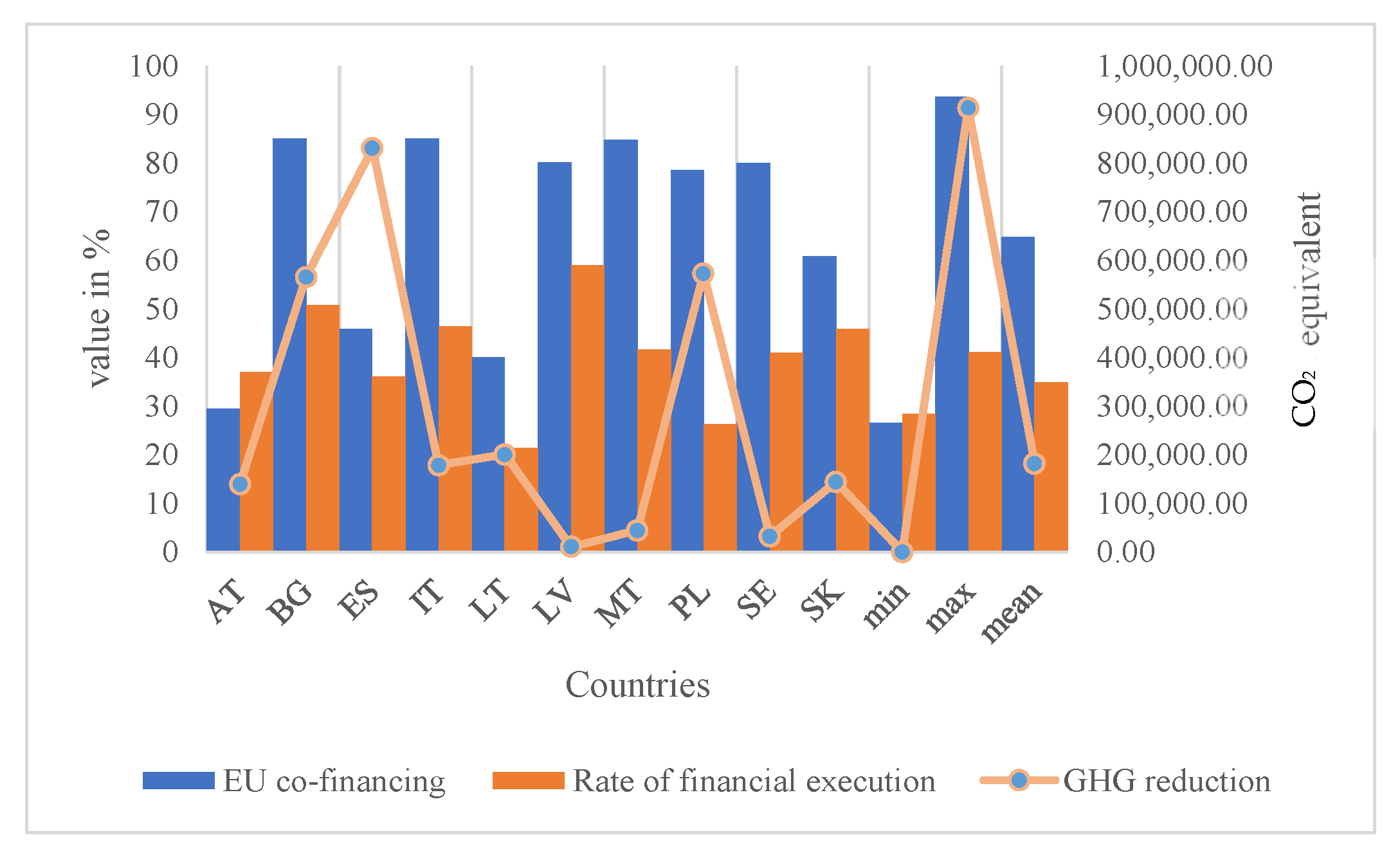
Most real-life applications are subject to uncertainty, and its presence is a challenge for most conventional DEA models, as it can influence efficiency results. Many researchers have already given special attention to the sensitivity of the results to data perturbations and to the study of the robustness of the efficiency scores resulting from these perturbations, considering the concept of super-efficiency in DEA models [36]. In the VBDEA, we assume the uncertainty in the coefficients of each criterion reflected through interval coefficients. Because the conventional super-efficiency DEA models are oriented, some infeasibility problems may arise. Since the VBDEA projects the inefficient DMUs in any direction in a way that minimizes the distance to the best of all, no infeasibility problems emerge [36]. To perform a robustness analysis, we consider perturbations in the coefficients of each criterion within an interval in a way that the value $p_{cj}$ (performance of DMU_j in criterion c is the nominal value within the range $p_{cj}^L\le p_{cj}\le p_{cj}^U$). The same tolerance δ is applied to all performances, in original values, such that $p_{cj}^L=p_{cj}\left(1-\delta \right)\le p_{cj}\le p_{cj}\left(1+\delta \right)=p_{cj}^U$. The value functions $v_c(.)$ are monotonous, and the following inequalities $v_c^L\left(DM{U}_j\right)\le v_c\left(DM{U}_j\right)\le v_c^U\left(DM{U}_j\right)$ are considered, if the criterion c is to be maximized, or $v_c^L\left(DM{U}_j\right)\ge v_c\left(DM{U}_j\right)\ge v_c^U\left(DM{U}_j\right)$, if the criterion c is to be minimized. With this procedure, it is possible to compute an optimistic efficiency measure and a pessimistic efficiency measure. Problem (1) can thus be changed to compute the optimistic efficiency measure considering the best value of the intervals for the DMU_k under evaluation and the worst value of the intervals for all the other DMUs, and the reverse is considered to compute the pessimistic efficiency measure. Thus, to compute the optimistic efficiency measure $d_k^{op{t}^{*}}$ for DMU_k, we solve Problem (3).

$$\begin{array}{l}\underset{d_k,w}{\min }{d}_k^{opt}\\ s.t. {\displaystyle \sum _{c=1}^q}{w}_c{v}_c^L\left(DM{U}_j\right)-{\displaystyle \sum _{c=1}^q}{w}_c{v}_c^U\left(DM{U}_k\right)\le d_k^{opt}, j=1,\dots ,n;j\ne k, \\ \sum _{c=1}^q{w}_c=1,\\ w_c\ge 0, \forall c=1,\dots ,q.\end{array}$$

(3)

To compute the pessimistic efficiency measure $d_k^{pe{s}^{*}}$ for $DM{U}_k$, we solve Problem (4).

$$\begin{array}{l}\underset{d_k,w}{\min }{d}_k^{pes}\\ s.t. {\displaystyle \sum _{c=1}^q}{w}_c{v}_c^U\left(DM{U}_j\right)-{\displaystyle \sum _{c=1}^q}{w}_c{v}_c^L\left(DM{U}_k\right)\le d_k^{pes}, j=1,\dots ,n;j\ne k, \\ \sum _{c=1}^q{w}_c=1,\\ w_c\ge 0, \forall c=1,\dots ,q.\end{array}$$

(4)

Problems (3) and (4) are solved after the original performances of the criteria are converted into value scales. With the scores $d_k^{op{t}^{*}}$ and $d_k^{pe{s}^{*}},$ it is possible to classify the DMUs as surely (i.e., robustly) efficient, potentially efficient, or surely (i.e., robustly) inefficient, for a given tolerance value.

4. Data

The choice of the indicators employed herein was inspired by [2]. The values considered are cumulative (referring to the programmatic period of 2014–2020) at the MS level from different years referring to ERDF devoted to an LCE, disclosed on 19 November 2021, as these are the most up-to-date data available for the achievement indicators. The study carried out considered only countries with complete information on ERDF. The criteria considered to evaluate the efficiency of the implementation of the funds were selected from the list of common indicators legally required by the EU [38] and are described below (see

Table 2. Criteria selected.

	EU Co-Financing	Total Eligible Spending	Eligible Cost Decided	GHG Reduction
Description	Percentage of EU financing (calculated as an average)	Eligible costs validated	Financial resources assigned	Estimated annual decrease in GHG
Type of factor	To minimize	To maximize	To minimize	To maximize
Unit	%	Euro	Euro	Tons of CO2 equivalent
Source	(a)	(a)	(a)	(b), (c)
Explanation	Considers concerns with the financial absorption capacity of the country or region	Reflects concerns about the pace of programs’ implementation	Reflects concerns about the pace of programs’ implementation	Reflects concerns on LCE

(a) List of Structural Funds financial implemented data. Available at: https://cohesiondata.ec.europa.eu/2014-2020/ESIF-2014-2020-Finance-Implementation-Details/99js-gm52, accessed on 1 July 2022. (b) List of common indicators legally required and listed in the annexes to the ERDF, Cohesion Fund, and ETC regulations. Available at: https://ec.europa.eu/regional_policy/sources/docoffic/2014/working/wd_2014_en.pdf, accessed on 1 July 2022. (c) List of Structural Funds achievement data. Available at: https://cohesiondata.ec.europa.eu/2014-2020/ESIF-2014-2020-Achievement-Details/aesb-873i, accessed on 1 July 2022.

).

Data on these factors are given in

Table 3. Data in their original performances.

DMU Number	Country Name (DMU) *	EU Co-Financing X1	Eligible Cost Decided X2	Total Eligible Spending Y1	GHG Reduction Y2
1	AT	29.46	1,128,573,111.00	417,572,434.00	138,916.85
2	BE	40.00	1,740,681,178.00	321,181,746.00	37.16
3	BG	85.00	576,761,290.00	292,362,689.00	564,998.70
4	CY	67.50	636,202,801.00	186,165,272.00	8242.96
5	CZ	57.36	14,373,000,000.00	4,962,960,249.00	82,646.53
6	DE	55.00	264,194,403.00	55,493,280.70	250,200.12
7	DK	65.56	10,150,000,000.00	4,032,596,628.00	51,005.00
8	ES	45.85	14,394,000,000.00	5,196,850,673.00	829,915.74
9	FR	76.25	6,896,424,047.00	2,409,491,434.00	349,456.89
10	GR	73.33	4,043,109,664.00	1,182,075,658.00	74,734.47
11	HU	50.00	932,612,037.00	399,673,586.00	71,538.06
12	IE	56.18	17,105,000,000.00	5,379,496,576.00	225,317.00
13	IT	85.00	3,453,293,427.00	1,600,903,861.00	177,850.29
14	LT	40.00	132,573,817.00	28,265,375.00	200,179.00
15	LU	85.00	1,694,042,534.00	443,556,817.00	838.00
16	LV	80.00	180,885,601.00	106,654,988.00	10,412.53
17	MT	84.63	16,871,000,000.00	7,016,881,169.00	44,352.40
18	PL	78.58	948,142,198.00	247,997,568.00	572,469.13
19	PT	83.75	7,505,375,116.00	1,371,781,717.00	2,648.16
20	RO	48.75	1,667,053,033.00	571,461,318.00	81,269.68
21	SE	79.97	99,506,488.00	40,727,849.30	31,796.00
22	SK	60.74	3,268,602,897.00	1,497,980,442.00	143,827.12
23	UK	59.07	7,012,247,172.00	2,356,033,638.00	256,424.84
	min	26.52	89,555,839.17	25,438,837.48	33.44
	max	93.50	18,815,551,238.00	7,718,569,286.00	912,907.30
	mean	64.65	5,003,198,869.00	1,744,268,042.00	181,264.20

* The acronyms for each MS are as follows: AT—Austria; BE—Belgium; BG—Bulgaria; CY—Cyprus; CZ—the Czech Republic; DE—Germany; DK—Denmark; ES—Spain; FR—France; GR—Greece; HU—Hungary; IE—Ireland; IT—Italy; LT—Lithuania; LU—Luxemburg; LV—Latvia; MT—Malta; PL—Poland; PT—Portugal; RO—Romania; SE—Sweden; SK—Slovakia; UK—the United Kingdom.

.

5. Discussion of Results

Although we may choose non-linear value functions with VBDEA, since we did not have a real DM, we transformed all the criteria into linear value functions.

To convert the factors into a value scale, we established two limits, $M_c^L$ and $M_c^U,$ to consider an acceptable higher tolerance value (in this case $\delta$= 10%). We chose $M_c^L<min\left\{p_{cj}^L,j=1,\dots ,n\right\}$ and $M_c^U>max\left\{p_{cj}^U,j=1,\dots ,n\right\}$ for each $c=1,\dots ,q$, to set the 0 and 1 levels on the value scales, according to the type of criteria (to maximize or minimize) (see Table 3). After that, we computed the values for each $DM{U}_j$, $j=1,\dots ,n$ using Expression (5):

$$v_c^{}\left(DM{U}_j\right)=\{\begin{array}{c}\frac{p_{cj}^{}-M_c^L}{M_c^U-M_c^L}, \mathrm{if} \mathrm{the} \mathrm{factor} c \mathrm{is} \mathrm{an} \mathrm{output}\\ \frac{M_c^U-p_{cj}^{}}{M_c^U-M_c^L}, \mathrm{if} \mathrm{the} \mathrm{factor} c \mathrm{is} \mathrm{an} \mathrm{output} \end{array}, j=1,\dots ,n; c =1,\dots ,q$$

(5)

We apply the VBDEA to the performance values in Table 3, and we obtain the results depicted in

Table 4. Data in value scales.

DMU Number	Country Name (DMU)	EU Co-Financing V1	Eligible Cost Decided V2	Total Eligible Spending V3	GHG Reduction V4
1	AT	0.9560	0.9445	0.0510	0.1521
2	BE	0.7987	0.9118	0.0384	0.0000
3	BG	0.1269	0.9740	0.0347	0.6189
4	CY	0.3882	0.9708	0.0209	0.0090
5	CZ	0.5395	0.2373	0.6418	0.0905
6	DE	0.5748	0.9907	0.0039	0.2740
7	DK	0.4171	0.4627	0.5209	0.0558
8	ES	0.7114	0.2361	0.6722	0.9091
9	FR	0.2575	0.6365	0.3099	0.3828
10	GR	0.3011	0.7889	0.1503	0.0818
11	HU	0.6494	0.9550	0.0486	0.0783
12	IE	0.5571	0.0913	0.6960	0.2468
13	IT	0.1269	0.8204	0.2048	0.1948
14	LT	0.7987	0.9977	0.0004	0.2192
15	LU	0.1269	0.9143	0.0543	0.0009
16	LV	0.2015	0.9951	0.0106	0.0114
17	MT	0.1324	0.1038	0.9088	0.0485
18	PL	0.2227	0.9542	0.0289	0.6271
19	PT	0.1456	0.6040	0.1750	0.0029
20	RO	0.6681	0.9158	0.0710	0.0890
21	SE	0.2020	0.9995	0.0020	0.0348
22	SK	0.4890	0.8302	0.1914	0.1575
23	UK	0.5140	0.6303	0.3029	0.2809

.

Phase 1 (Problem (1)) returns the efficiency measure, d_k*, for each DMU_k, k = 1, …, n, and the corresponding weighting vector. In Phase 2, Problem (2) is solved only for inefficient DMUs, and a proposal of an efficiency target (projection) for each inefficient DMU is obtained. To reach an efficiency status, these inefficient DMUs must change their value in each factor by the amount indicated by the slack (s*). The results (in

Table 5. Efficiency score, weights, slacks, and reference DMUs obtained according to the VBDEA method.

		Phase 1					Phase 2
Number	DMUs	d*	w1	w2	w3	w4	s1	s2	s3	s4	λ1	λ3	λ8	λ13	λ14	λ16	λ17	λ22
1	AT	−0.157	1.000	0.000	0.000	0.000
2	BE	0.025	0.019	0.507	0.475	0.000	0.157	0.033	0.013	0.152	1.000	0.000	0.000	0.000	0.000	0.000	0.000	0.000
3	BG	−0.017	0.000	0.904	0.000	0.096
4	CY	0.007	0.006	0.525	0.469	0.000	0.000	0.013	0.000	0.071	0.000	0.000	0.000	0.000	0.277	0.650	0.000	0.073
5	CZ	0.034	0.112	0.395	0.494	0.000	0.184	0.034	0.000	0.782	0.049	0.000	0.951	0.000	0.000	0.000	0.000	0.000
6	DE	0.003	0.000	0.649	0.341	0.009	0.132	0.004	0.001	0.000	0.000	0.137	0.000	0.000	0.863	0.000	0.000	0.000
7	DK	0.013	0.033	0.472	0.495	0.000	0.088	0.021	0.000	0.040	0.452	0.000	0.000	0.000	0.000	0.000	0.548	0.000
8	ES	−0.413	0.000	0.000	0.363	0.637
9	FR	0.028	0.028	0.452	0.478	0.043	0.000	0.061	0.000	0.000	0.000	0.451	0.056	0.000	0.000	0.000	0.226	0.267
10	GR	0.042	0.003	0.524	0.473	0.000	0.000	0.036	0.048	0.095	0.000	0.000	0.000	0.519	0.000	0.000	0.000	0.481
11	HU	0.001	0.006	0.525	0.469	0.000	0.000	0.000	0.001	0.101	0.000	0.000	0.000	0.000	0.628	0.119	0.000	0.253
12	IE	0.028	0.290	0.000	0.710	0.000	0.096	0.132	0.000	0.576	0.000	0.000	0.900	0.000	0.000	0.000	0.100	0.000
13	IT	−0.002	0.000	0.487	0.496	0.017
14	LT	−0.030	0.108	0.892	0.000	0.000
15	LU	0.022	0.003	0.524	0.473	0.000	0.045	0.042	0.000	0.560	0.000	0.875	0.000	0.000	0.000	0.000	0.000	0.125
16	LV	−0.001	0.003	0.557	0.440	0.000
17	MT	−0.213	0.000	0.000	1.000	0.000
18	PL	−0.019	0.235	0.350	0.000	0.416
19	PT	0.122	0.005	0.493	0.502	0.000	0.232	0.000	0.240	0.121	0.000	0.000	0.000	0.000	0.000	0.000	0.311	0.689
20	RO	0.010	0.019	0.507	0.475	0.000	0.170	0.000	0.015	0.065	0.748	0.000	0.000	0.000	0.000	0.000	0.000	0.252
21	SE	−0.002	0.000	1.000	0.000	0.000
22	SK	−0.005	0.019	0.486	0.495	0.000
23	UK	0.031	0.034	0.449	0.478	0.039	0.000	0.069	0.000	0.000	0.005	0.000	0.170	0.000	0.000	0.000	0.042	0.783

) classify 10 countries as efficient (with d_k* ≤ 0—see the values in red) corresponding to Spain (DMU 8), Malta (DMU 17), Austria (DMU 1), Lithuania (DMU 14), Polonia (DMU 18), Bulgaria (DMU 3), Slovakia (DMU 22), Italy (DMU 13), Sweden (DMU 21), and Latvia (DMU 16). The best of all, i.e., with the most negative score, is Spain, followed by Malta and Austria. These three countries have efficiency levels far from the other efficient countries; therefore, they are the most robust in the group of efficient countries.

The three countries more often selected as benchmarks in terms of best practices for the non-efficient countries are Slovakia (eight times), Malta (five times), and Austria (five times)—see Figure 2.

Figure 2. Number of times the countries are viewed as benchmarks.

Figure 2. Number of times the countries are viewed as benchmarks.

The factor most valued by the countries to achieve the best possible classification, when compared to the others, was the “Eligible cost decided” (w2), followed by the “Total eligible spending” (w3) (Figure 3). However, none of the top three countries, in terms of their efficiency score, chose to consider the factor “Eligible cost decided”. In fact, Spain only gave importance to the outputs (“Total eligible spending” and “GHG reduction”) to rank first (w3 = 0.363 and w4 = 0.637). Malta only considered “Total eligible spending” (w3 = 1), disregarding all the other factors, and Austria valued only “EU co-financing” (w1 = 1), to position itself in third place (see Table 4). Out of the 10 efficient countries, only 4 (Bulgaria, Spain, Italy, and Poland) elected “GHG reduction” as a criterion relevant to attaining efficiency. In addition, it is interesting to see two out of the four Visegrad countries as efficient in the implementation of ERDF devoted to an LCE, with one of them more frequently elected as a reference for best practices. Finally, it is also interesting to see that except for Poland and Lithuania, all efficient countries managed to attain a higher-than-average financial execution rate (i.e., the ratio between total eligible spending and total costs decided)—see Figure 4.

Figure 3. Weights chosen by all DMUs (a) and by efficient DMUs (b). Note: w1 refers to “EU co-financing”, w2 refers to “Eligible costs decided”, w3 refers to “Total eligible spending”, and w4 refers to “GHG reduction”.

Figure 3. Weights chosen by all DMUs (a) and by efficient DMUs (b). Note: w1 refers to “EU co-financing”, w2 refers to “Eligible costs decided”, w3 refers to “Total eligible spending”, and w4 refers to “GHG reduction”.

Figure 4. Data on the efficient countries.

Figure 4. Data on the efficient countries.

Table 5 also shows the results for the countries with a positive efficiency score, which are classified as inefficient. The more positive the efficiency score, the more inefficient the countries (i.e., the distance to the best of all DMUs is getting bigger). Portugal (DMU 19), Greece (DMU 10), and the Czech Republic (DMU 5) are the most inefficient countries. In Phase 2, the optimal weighting vector w*∈W is used to solve the problem in formulation (2). The solution is a proposed efficiency target for each inefficient country and the adjustments that are needed to achieve that target. According to Figure 5, the biggest adjustments should be made at the level of the output “GHG reduction”, followed by the input “EU co-financing”.

Figure 5. Adjustments required of inefficient countries given by the slacks.

Figure 5. Adjustments required of inefficient countries given by the slacks.

The Czech Republic is the country that needs to make the biggest “GHG reduction” of all countries in the sample, followed by Ireland and Luxembourg. There are only three inefficient countries that do not require a “GHG reduction”, which are Germany, France, and the UK. All these countries are mainly inefficient because they are overusing EU funding devoted to the promotion of LCE. In the case of Germany and France, they consider a strong climate policy to be advantageous to their economic development [39].

5.1. Introduction of Constraints on the Weights Ranking Order

When allowed to freely choose their weights, there are countries that neglect some criteria in the evaluation performed with the VBDEA model (see the previous section). Hence, by establishing a different ranking of the weights according to two potential political concerns, it is ensured that none of the factors is disregarded from the assessment. We consider two sets of weight constraints that allow reflecting two different policy scenarios. Since the financial execution of ESIF is a fundamental requirement for efficient policy execution, the first scenario is more focused on the financial rate of execution of the funds, whereas the second scenario is more focused on environmental concerns. Therefore, the following ranking orders of the weights were added to Phase 1 and Phase 2 of the VBDEA method for the first and second scenarios, respectively: w3 ≥ w4 ≥ w2 ≥ w1 and w4 ≥ w3 ≥ w2 ≥ w1.

After introducing the first set of weights, which reflects the priority of increasing the “Total eligible spending” (Scenario 1), we obtain the results depicted in

Table 6. Efficiency score, weights, slacks, and benchmarks obtained with weight restrictions (Scenario 1).

	Phase 1					Phase 2
DMUs	d*	w1	w2	w3	w4	s1	s2	s3	s4	λ8	λ17
AT	0.106	0.250	0.250	0.250	0.250	−0.245	−0.708	0.621	0.757	1.000	0.000
BE	0.195	0.250	0.250	0.250	0.250	−0.087	−0.676	0.634	0.909	1.000	0.000
BG	0.065	0.003	0.332	0.332	0.332	0.584	−0.738	0.638	0.290	1.000	0.000
CY	0.272	0.003	0.332	0.332	0.332	0.323	−0.735	0.651	0.900	1.000	0.000
CZ	0.124	0.104	0.104	0.689	0.104	0.172	−0.001	0.030	0.819	1.000	0.000
DE	0.171	0.250	0.250	0.250	0.250	0.137	−0.755	0.668	0.635	1.000	0.000
DK	0.200	0.104	0.104	0.689	0.104	0.294	−0.227	0.151	0.853	1.000	0.000
ES	−0.313	0.017	0.017	0.483	0.483
FR	0.164	0.003	0.332	0.332	0.332	0.454	−0.400	0.362	0.526	1.000	0.000
GR	0.266	0.003	0.332	0.332	0.332	0.410	−0.553	0.522	0.827	1.000	0.000
HU	0.199	0.250	0.250	0.250	0.250	0.062	−0.719	0.624	0.831	1.000	0.000
IE	0.083	0.104	0.104	0.689	0.104	0.000	0.110	0.039	0.433	0.734	0.266
IT	0.200	0.003	0.332	0.332	0.332	0.584	−0.584	0.467	0.714	1.000	0.000
LT	0.128	0.250	0.250	0.250	0.250	−0.087	−0.762	0.672	0.690	1.000	0.000
LU	0.284	0.003	0.332	0.332	0.332	0.584	−0.678	0.618	0.908	1.000	0.000
LV	0.268	0.003	0.332	0.332	0.332	0.510	−0.759	0.662	0.898	1.000	0.000
MT	−0.201	0.010	0.010	0.971	0.010
PL	0.070	0.003	0.332	0.332	0.332	0.489	−0.718	0.643	0.282	1.000	0.000
PT	0.346	0.003	0.332	0.332	0.332	0.566	−0.368	0.497	0.906	1.000	0.000
RO	0.196	0.250	0.250	0.250	0.250	0.043	−0.680	0.601	0.820	1.000	0.000
SE	0.261	0.003	0.332	0.332	0.332	0.509	−0.763	0.670	0.874	1.000	0.000
SK	0.213	0.003	0.332	0.332	0.332	0.222	−0.594	0.481	0.752	1.000	0.000
UK	0.200	0.250	0.250	0.250	0.250	0.197	−0.394	0.369	0.628	1.000	0.000

. From Figure 6a, it can be established that regarding the efficient countries without the weight constraints, only two manage to maintain their efficiency: Spain and Malta (d1* < 0—see the values in red). While Spain assigned similar weights to both “Total eligible spending” and “GHG reduction” (w3 = w4 = 0.483, Figure 6a, against the previous w3 = 0.363 and w4 = 0.637, Figure 3b) to justify its efficiency, Malta keeps assigning the highest weight to “Total eligible spending” (w3 = 0.971 and w4 = 0.1, Figure 6a, against the previous values of w3 = 1 and w4 = 0, Figure 3b). All the other previously efficient countries (in the Original Scenario) became inefficient but now manage to assign values to w3 = w4 between 0.25 and 0.332. While in the case of Austria and Lithuania the weights are evenly distributed across all criteria (i.e., w1 = w2 = w3 = w4 = 0.25), in the remaining countries, the “EU co-funding” receives a minor weight (w1 = 0.003) for justifying their best efficiency outcomes, suggesting that the values of this criterion have a detrimental effect on efficiency for these latter countries.

Figure 6. Weights chosen by efficient countries under Scenarios 1 (a) and 2 (b). Note: w1 refers to “EU co-financing”, w2 refers to “Eligible costs decided”, w3 refers to “Total eligible spending”, and w4 refers to “GHG reduction”.

Figure 6. Weights chosen by efficient countries under Scenarios 1 (a) and 2 (b). Note: w1 refers to “EU co-financing”, w2 refers to “Eligible costs decided”, w3 refers to “Total eligible spending”, and w4 refers to “GHG reduction”.

In some cases, for inefficient countries to be able to match their peers on the efficiency frontier, negative slacks arise (see the case of “Eligible costs decided”), particularly in the criteria being minimized, suggesting that rather than decreasing and enhancing these criteria, they should be worsened—see Figure 7.

Figure 7. Average values for efficiency and for all the required adjustments (slacks) without constraints and for Scenarios 1 and 2. Note: s1 refers to “EU co-financing”, s2 refers to “Eligible costs decided”, s3 refers to “Total eligible spending”, and s4 refers to “GHG reduction”.

Figure 7. Average values for efficiency and for all the required adjustments (slacks) without constraints and for Scenarios 1 and 2. Note: s1 refers to “EU co-financing”, s2 refers to “Eligible costs decided”, s3 refers to “Total eligible spending”, and s4 refers to “GHG reduction”.

Most countries, except for Ireland, have negative slacks (see the values in red of Phase 2) associated with “Eligible cost decided”, which means that to reach the efficient frontier and to follow the same practices of their corresponding benchmark (Spain), the “Eligible cost decided” should be increased by the absolute value indicated in the slacks, and all the other factors should also be adjusted in accordance (see Table 6).

For instance, in the case of Austria, to reach its benchmark (Spain), both inputs should be increased (s1 = −0.245 and s2 = −0.708), i.e., both the percentage of “EU co-funding” and the amount of ERDF devoted to LCE (“Total costs decided”), and, at the same time, it should also increase “Total eligible spending” and the amount of “GHG reduction” (s3 = 0.621 and s4 = 0.757).

These findings suggest that, in general, there is still plenty of room for improvement regarding the financial execution of ERDF committed to an LCE, but this would require an average significant increase in both “Total costs decided” and “Total eligible spending”—see Figure 7. Note that the average performance in terms of “GHG reduction” must also suffer a substantial increase when contrasted with the original situation without the weight constraints, even if this is not a priority in this scenario—see Figure 6 and Figure 7.

After introducing the second set of weights, which reflects the focus on “GHG reduction” (Scenario 2), only Spain becomes efficient—see

Table 7. Efficiency score, weights, slacks, and reference DMUs obtained with weight restrictions (Scenario 2).

	Phase 1					Phase 2
DMUs	d*	w1	w2	w3	w4	s1	s2	s3	s4	λ8
AT	0.106	0.250	0.250	0.250	0.250	−0.245	−0.708	0.621	0.757	1.000
BE	0.195	0.250	0.250	0.250	0.250	−0.087	−0.676	0.634	0.909	1.000
BG	0.065	0.003	0.332	0.332	0.332	0.584	−0.738	0.638	0.290	1.000
CY	0.272	0.003	0.332	0.332	0.332	0.323	−0.735	0.651	0.900	1.000
CZ	0.255	0.250	0.250	0.250	0.250	0.172	−0.001	0.030	0.819	1.000
DE	0.171	0.250	0.250	0.250	0.250	0.137	−0.755	0.668	0.635	1.000
DK	0.259	0.003	0.332	0.332	0.332	0.294	−0.227	0.151	0.853	1.000
ES	−0.408	0.006	0.006	0.362	0.626
FR	0.164	0.003	0.332	0.332	0.332	0.454	−0.400	0.362	0.526	1.000
GR	0.266	0.003	0.332	0.332	0.332	0.410	−0.553	0.522	0.827	1.000
HU	0.199	0.250	0.250	0.250	0.250	0.062	−0.719	0.624	0.831	1.000
IE	0.234	0.250	0.250	0.250	0.250	0.154	0.145	−0.024	0.662	1.000
IT	0.200	0.003	0.332	0.332	0.332	0.584	−0.584	0.467	0.714	1.000
LT	0.128	0.250	0.250	0.250	0.250	−0.087	−0.762	0.672	0.690	1.000
LU	0.284	0.003	0.332	0.332	0.332	0.584	−0.678	0.618	0.908	1.000
LV	0.268	0.003	0.332	0.332	0.332	0.510	−0.759	0.662	0.898	1.000
MT	0.253	0.003	0.332	0.332	0.332	0.579	0.132	−0.237	0.861	1.000
PL	0.070	0.003	0.332	0.332	0.332	0.489	−0.718	0.643	0.282	1.000
PT	0.346	0.003	0.332	0.332	0.332	0.566	−0.368	0.497	0.906	1.000
RO	0.196	0.250	0.250	0.250	0.250	0.043	−0.680	0.601	0.820	1.000
SE	0.261	0.003	0.332	0.332	0.332	0.509	−0.763	0.670	0.874	1.000
SK	0.213	0.003	0.332	0.332	0.332	0.222	−0.594	0.481	0.752	1.000
UK	0.200	0.250	0.250	0.250	0.250	0.197	−0.394	0.369	0.628	1.000

and Figure 6b. In this case, only Ireland and Malta are allowed to worsen the “Total eligible expending” to match their benchmark (Spain). Note that these two countries have negative output slacks for this criterion. Hence, Ireland needs to improve (i.e., reduce) its inputs (s1 = 0.154 and s2 = 0.145); it can slightly worsen the output “Total eligible expenses” (s3 = −0.024), but it needs to tremendously improve (i.e., increase) the output “GHG reduction” (s4 = 0.662).

By comparing the two scenarios derived from the introduction of the weight constraints, we can conclude that when environmental concerns are a major source of concern, countries such as Malta (efficient in Scenario 1 and in the Original Scenario—always privileged financial execution in these two scenarios), Denmark (never efficient—always privileged financial execution in Scenario 1 and the Original Scenario), the Czech Republic (never efficient—always privileged financial execution in Scenario 1 and the Original Scenario), and Ireland (never efficient—always privileged financial execution in Scenario 1 and in Original Scenario) lose efficiency. Spain (always efficient—always privileged environmental concerns) is the only country that improves the efficiency score when environmental concerns are explicitly addressed (see Figure 8).

Figure 8. Efficiency scores with and without weight constraints.

Figure 8. Efficiency scores with and without weight constraints.

All in all, as was expected, by introducing these new weight constraints, the efficiency scores of most of the countries become worse, particularly in Scenario 2, highlighting the importance that “GHG reduction” has on efficiency (see Table 6 and Table 7). In addition, the highest adjustments required to attain efficiency across all scenarios always highlight the importance of attaining a significant improvement in “GHG reduction”.

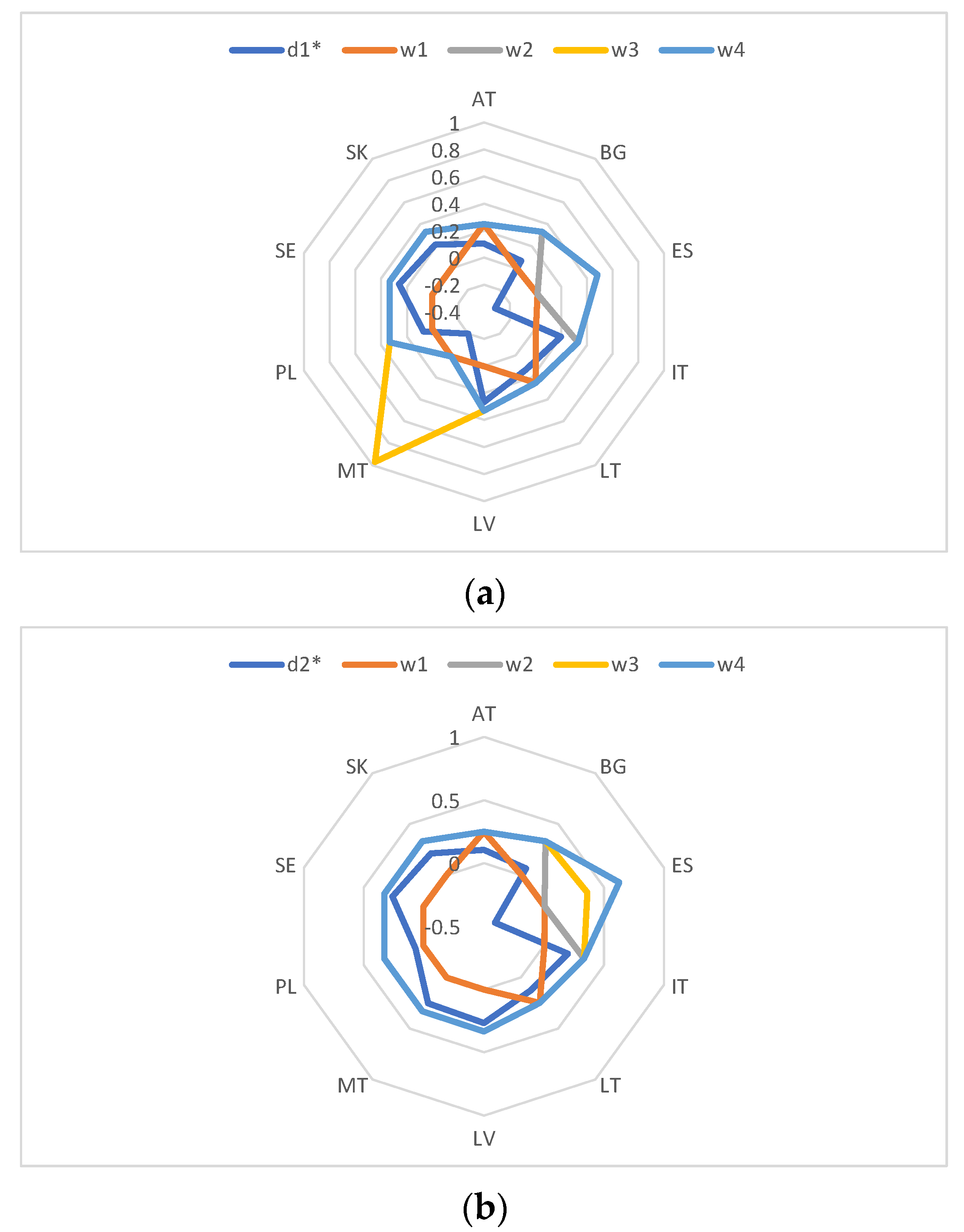
5.2. Robustness Analysis Results

We perform a robustness analysis of the efficiency scores for each DMU, considering a tolerance of δ = 5% and δ = 10%. The lower limit is obtained from the solution of Problem (3), and the upper limit is the solution of Problem (4). The results are exhibited in

Table 8. Lower and upper limits for the utility loss [$d_k^{op{t}^{*}}$, $d_k^{pe{s}^{*}}$], for each DMU.

		5%		10%
DMUs	Countries	$$d_k^{op{t}^{*}}$$	$$d_k^{pe{s}^{*}}$$	$$d_k^{op{t}^{*}}$$	$$d_k^{pe{s}^{*}}$$
1	AT	−0.206	−0.104	−0.257	−0.053
2	BE	0.018	0.033	0.010	0.041
3	BG	−0.046	−0.008	−0.096	−0.003
4	CY	0.003	0.010	0.000	0.014
5	CZ	−0.038	0.106	−0.108	0.178
6	DE	0.001	0.004	−0.026	0.006
7	DK	−0.042	0.067	−0.097	0.121
8	ES	−0.475	−0.351	−0.543	−0.290
9	FR	−0.009	0.064	−0.045	0.101
10	GR	0.023	0.061	0.004	0.080
11	HU	−0.005	0.006	−0.011	0.012
12	IE	−0.046	0.102	−0.120	0.177
13	IT	−0.022	0.017	−0.042	0.037
14	LT	−0.040	−0.022	−0.055	−0.013
15	LU	0.014	0.029	0.006	0.037
16	LV	−0.003	0.000	−0.004	0.001
17	MT	−0.293	−0.132	−0.374	−0.052
18	PL	−0.075	0.017	−0.131	0.022
19	PT	0.092	0.151	0.064	0.181
20	RO	0.001	0.019	−0.008	0.028
21	SE	−0.002	−0.001	−0.003	−0.001
22	SK	−0.025	0.015	−0.045	0.035
23	UK	−0.005	0.066	−0.040	0.102

.

Austria (DMU 1), Bulgaria (DMU 3), Spain (DMU 8), Malta (DMU 17), Lithuania (DMU 14), and Sweden (DMU 21) are surely efficient and remain with this status for both tolerances considered (5% and 10%). Belgium (DMU 2), Cyprus (DMU 4), Greece (DMU 10), Luxembourg (DMU 15), and Portugal (DMU 19) are surely inefficient if the uncertainty intervals are set according to tolerances of 5% and 10%. Latvia is surely efficient for a tolerance of 5%, but potentially efficient when a perturbation of 10% in all factors is considered. Germany and Romania are surely inefficient for a tolerance of 5% and potentially efficient for a tolerance of 10%. All the other countries are potentially efficient for both tolerance values. With this analysis, it is possible to see that the threshold for Spain to lose its efficient status is higher in relation to the others. This country is the most robustly efficient of all. Slovakia, the more often chosen as a benchmark (see Figure 1) for the inefficient countries is only potentially efficient, for both tolerance values.

6. Conclusions and Further Research

The main objective of this paper was to evaluate the efficiency of the implementation of the ERDF devoted to the support of an LCE in 23 EU MS. We suggest a three-stage VBDEA modeling approach to achieve this goal.

Unlike other alternative methods applied in comparable situations, the VBDEA model is particularly important for MA, as it enables, within a single stage, ranking all the OPs (either efficient or inefficient) under evaluation, helping in the identification of the reasons behind their (in)efficiency. Besides allowing to include the preference of the DMs, this model also enables tackling the null and negative data easily because it relies on the use of value functions to translate the DMs’ preferences.

The answers to our main research questions are given below.

RQ1: “What are the criteria mainly responsible for the in(efficient) use of ERDF allocated to boost an LCE in EU MS?”

The criteria most sought to attain the greatest efficiency score possible were “Eligible cost decided” followed by “Total eligible spending”. Furthermore, just four out of the ten efficient countries (Bulgaria, Spain, Italy, and Poland) choose “GHG reduction” as an important criterion for achieving efficiency. On the other hand, the most substantial improvements needed to achieve efficiency for inefficient countries should be undertaken at the level of “GHG reduction” and “EU co-financing”. This suggests that for inefficient countries, there should be a major concern both regarding the choice of projects that lead to GHG reduction and the dependence on EU subsidies.

RQ2: “Which MS were viewed as benchmarks throughout the programming period?”

The countries ranked as the top four most often selected as benchmarks were Slovakia (eight times), followed ex aequo by Austria and Malta (five times), Spain (four times), Bulgaria and Lithuania (three times), and Latvia (two times).

RQ3: “How does efficiency change with the introduction of a hypothetical DM’s political preferences?”

Based on our findings, Spain was the only country that remained efficient across all scenarios, whereas Malta was able to maintain its efficiency only in Scenario 1. All the countries that lost their efficiency status from Scenarios 1 to 2 prioritized their financial execution to achieve efficiency. Our findings corroborate the robustness of Spain in terms of efficiency since this country seems to be immune to the scenarios considered. Finally, the most drastic changes necessary to achieve efficiency across all scenarios usually emphasize the significance of achieving a large improvement in “GHG reduction”.

While in the Original Scenario, most of the EU MS that have successfully been adopting renewables, such as Germany, France, and Italy, did not need to further reduce GHG emissions to attain efficiency, with the inclusion of the weight constraints, this condition no longer holds. Notably, all of these countries prioritized the financial execution of ERDF in the Original Scenario, further highlighting the true reasons behind the importance of economic concerns involved in the investment in LCE. Finally, the two Visegrad countries (Poland and Slovakia) that previously reached efficiency, lose their efficient status. In the case of Slovakia that was more often viewed as a reference for best practices (in the Original Scenario), this is particularly evident because of the significant required reduction in GHG emissions in Scenarios 1 and 2, while Poland, which already had a good performance of this indicator, only needs a mild reduction.

RQ4: “Which MS demonstrate a higher robustness performance in the face of data changes?”

Austria (DMU 1), Bulgaria (DMU 3), Spain (DMU 8), Malta (DMU 17), Lithuania (DMU 14), and Sweden (DMU 21) are robustly efficient and remain like this for both tolerances (5% and 10%). Belgium (DMU 2), Cyprus (DMU 4), Greece (DMU 10), Luxembourg (DMU 15), and Portugal (DMU 19) are robustly inefficient within both tolerances of 5% and 10%. Latvia is robustly efficient for a tolerance of 5% but potentially efficient for a tolerance of 10%. Germany and Romania are robustly inefficient for a tolerance of 5% and potentially efficient for a tolerance of 10%. All the remaining countries are potentially efficient for both tolerances.

All in all, it is possible to conclude that Spain is the most robustly efficient country. On the other hand, although Slovakia is more often viewed as a benchmark, it is only potentially efficient for both tolerances.

In summary, our findings show that most of the EU MS that have effectively been deploying renewables (see, e.g., Germany (inefficient), Spain (efficient), France (inefficient), and Italy (efficient)), when efficient in the use of ERDF devoted to an LCE, value the reduction in GHG emissions to attain their efficiency, and when inefficient, do not need to further reduce GHG emissions to become efficient, being considered as over-users of these sort of EU funds. These countries tend to perceive the investment in LCE (namely, the increase in renewable deployment) as a business and industrial prospect, which allows them to diversify their energy portfolio, also decreasing energy imports. The bulk of these MS are in Western Europe and have bigger GDPs, more established energy markets, and superior infrastructure. Because their citizens have better salaries, they are less vulnerable to increases in energy prices and are willing to pay a premium price to prevent larger environmental responsibilities. Moreover, these nations employ a considerable amount of their workers in the renewable energy industry, which provides them with economic advantages despite increased taxes and levies [40]. Moreover, it is curious to see a positive shift in two Visegrad countries (Poland and Slovakia) which were traditionally resisting an LCE transition. In fact, the Visegrad countries had organized action against both the EU renewable energy directives and the EU electricity market reforms [40]. Note also that these countries were very exposed to energy supply disturbances, were extremely reliant on oil, regularly depended on Russia as a single supplier, and are situated on the periphery of the EU. Hence, this shift in attitude toward the adoption of an LCE, particularly in the case of Poland, Slovakia, and other Eastern EU countries, such as Latvia, Lithuania, and Bulgaria, might be partially explained by the Crimea annexation in 2014 (the time horizon of this analysis is 2014–2020). However, other countries such as Romania, Hungary, and the Czech Republic did not manage to implement these funds efficiently. Considering these results, the EU still needs to promote policies that guarantee economic benefits from investing in an LCE, particularly for countries with fewer resources, offering these countries better financial conditions and know-how.

One of the major difficulties of this study referred to the lack of data reported, hence resulting in the use of fewer criteria and countries.

Future work should assess the evolution of the productivity of ERDF in the TO under assessment, also, eventually, involving real DMs.

References

1. Hanna, R.; Xu, Y.; Victor, D.G. After COVID-19, green investment must deliver jobs to get political traction. Nature 2020, 582, 178–180. [Google Scholar] [CrossRef] [PubMed]
2. Henriques, C.; Viseu, C.; Trigo, A.; Gouveia, M.; Amaro, A. How Efficient Is the Cohesion Policy in Supporting Small and Mid-Sized Enterprises in the Transition to a Low-Carbon Economy? Sustainability 2022, 14, 5317. [Google Scholar] [CrossRef]
3. Gouveia, M.C.; Henriques, C.O.; Costa, P. Evaluating the efficiency of structural funds: An application in the competitiveness of SMEs across different EU beneficiary regions. Omega 2021, 101, 102265. [Google Scholar] [CrossRef]
4. Henriques, C.; Viseu, C.; Neves, M.; Amaro, A.; Gouveia, M.; Trigo, A. How Efficiently Does the EU Support Research and Innovation in SMEs? J. Open Innov. Technol. Mark. Complex. 2022, 8, 92. [Google Scholar] [CrossRef]
5. Zhang, J.; Zeng, W.; Wang, J.; Yang, F.; Jiang, H. Regional low-carbon economy efficiency in China: Analysis based on the Super-SBM model with CO2 emissions. J. Clean. Prod. 2017, 163, 202–211. [Google Scholar] [CrossRef]
6. Zheng, Z. Energy efficiency evaluation model based on DEA-SBM-Malmquist index. Energy Rep. 2021, 7, 397–409. [Google Scholar] [CrossRef]
7. Miaomiao, T.; Thye, G.L.; Chandran, G.V. The Role of Industrial Structure Adjustment in China’s Low-Carbon Eco-Efficiency: A Super-Slack-Based Measure (Super-SBM) Approach. Int. J. Econ. Manag. 2022, 16, 21–43. [Google Scholar]
8. Meng, M.; Qu, D. Understanding the green energy efficiencies of provinces in China: A Super-SBM and GML analysis. Energy 2022, 239, 121912. [Google Scholar] [CrossRef]
9. Ding, Y.; Han, Y. Low Carbon Economy Assessment in China Using the Super-SBM Model. Discret. Dyn. Nat. Soc. 2022, 2022, 4690140. [Google Scholar] [CrossRef]
10. Chenet, H.; Ryan-Collins, J.; van Lerven, F. Finance, climate-change and radical uncertainty: Towards a precautionary approach to financial policy. Ecol. Econ. 2021, 183, 106957. [Google Scholar] [CrossRef]
11. Liu, X.; Liu, J. Measurement of low carbon economy efficiency with a three-stage data envelopment analysis: A comparison of the largest twenty CO2 emitting countries. Int. J. Environ. Res. Public Health 2016, 13, 1116. [Google Scholar] [CrossRef] [PubMed]
12. He, X.; Zhang, J. Supplier selection study under the respective of low-carbon supply chain: A hybrid evaluation model based on FA-DEA-AHP. Sustainability 2018, 10, 564. [Google Scholar] [CrossRef]
13. Meng, M.; Fu, Y.; Wang, L. Low-carbon economy efficiency analysis of China’s provinces based on a range-adjusted measure and data envelopment analysis model. J. Clean. Prod. 2018, 199, 643–650. [Google Scholar] [CrossRef]
14. Zha, J.; He, L.; Liu, Y.; Shao, Y. Evaluation on development efficiency of low-carbon tourism economy: A case study of Hubei Province, China. Socio-Econ. Plan. Sci. 2019, 66, 47–57. [Google Scholar] [CrossRef]
15. Zhang, Y.; Shen, L.; Shuai, C.; Tan, Y.; Ren, Y.; Wu, Y. Is the low-carbon economy efficient in terms of sustainable development? A global perspective. Sustain. Dev. 2019, 27, 130–152. [Google Scholar] [CrossRef]
16. Lin, X.; Zhu, X.; Han, Y.; Geng, Z.; Liu, L. Economy and carbon dioxide emissions effects of energy structures in the world: Evidence based on SBM-DEA model. Sci. Total Environ. 2020, 729, 138947. [Google Scholar] [CrossRef]
17. Chen, Y.; Chen, M.; Li, T. China’s CO2 emissions reduction potential: A novel inverse DEA model with frontier changes and comparable value. Energy Strategy Rev. 2021, 38, 100762. [Google Scholar] [CrossRef]
18. Furlan, M.; Mariano, E. Guiding the nations through fair low-carbon economy cycles: A climate justice index proposal. Ecol. Indic. 2021, 125, 107615. [Google Scholar] [CrossRef]
19. Mwambo, F.M.; Fürst, C.; Martius, C.; Jimenez-Martinez, M.; Nyarko, B.K.; Borgemeister, C. Combined application of the EM-DEA and EX-ACT approaches for integrated assessment of resource use efficiency, sustainability and carbon footprint of smallholder maize production practices in sub-Saharan Africa. J. Clean. Prod. 2021, 302, 126132. [Google Scholar] [CrossRef]
20. Li, W.; Zhang, P. Developing the transformation of scientific and technological achievements in colleges and universities to boost the development of low-carbon economy. Int. J. Low-Carbon Technol. 2021, 16, 305–316. [Google Scholar] [CrossRef]
21. Song, Y.; Zhang, J.; Song, Y.; Fan, X.; Zhu, Y.; Zhang, C. Can industry-university-research collaborative innovation efficiency reduce carbon emissions? Technol. Forecast. Soc. Chang. 2020, 157, 120094. [Google Scholar] [CrossRef]
22. Wu, D.; Wang, Y.; Qian, W. Efficiency evaluation and dynamic evolution of China’s regional green economy: A method based on the Super-PEBM model and DEA window analysis. J. Clean. Prod. 2020, 264, 121630. [Google Scholar] [CrossRef]
23. Fu, Y.; He, C.; Luo, L. Does the low-carbon city policy make a difference? Empirical evidence of the pilot scheme in China with DEA and PSM-DID. Ecol. Indic. 2021, 122, 107238. [Google Scholar] [CrossRef]
24. Liang, G.; Yu, D.; Ke, L. An empirical study on dynamic evolution of industrial structure and green economic growth—Based on data from china’s underdeveloped areas. Sustainability 2021, 13, 8154. [Google Scholar] [CrossRef]
25. Shuai, S.; Fan, Z. Modeling the role of environmental regulations in regional green economy efficiency of China: Empirical evidence from super efficiency DEA-Tobit model. J. Environ. Manag. 2020, 261, 110227. [Google Scholar] [CrossRef]
26. Kutty, A.A.; Kucukvar, M.; Abdella, G.M.; Bulak, M.E.; Onat, N.C. Sustainability Performance of European Smart Cities: A Novel DEA Approach with Double Frontiers. Sustain. Cities Soc. 2022, 81, 103777. [Google Scholar] [CrossRef]
27. Liang, S.; Yang, J.; Ding, T. Performance evaluation of AI driven low carbon manufacturing industry in China: An interactive network DEA approach. Comput. Ind. Eng. 2022, 170, 108248. [Google Scholar] [CrossRef]
28. Xia, J.; Zhan, X.; Li RY, M.; Song, L. The Relationship Between Fiscal Decentralization and China’s Low Carbon Environmental Governance Performance: The Malmquist Index, an SBM-DEA and Systematic GMM Approaches. Front. Environ. Sci. 2022, 10, 945922. [Google Scholar] [CrossRef]
29. Wang, J.; Li, H.; Guo, H. Coordinated Development of Logistics Development and Low-Carbon Environmental Economy Base on AHP-DEA Model. Sci. Program. 2022, 2022, 5891909. [Google Scholar] [CrossRef]
30. Charnes, A.; Cooper, W.W.; Rhodes, E. Measuring the efficiency of decision making units. Eur. J. Oper. Res. 1978, 2, 429–444. [Google Scholar] [CrossRef]
31. Golany, B.; Roll, Y. An application procedure for DEA. Omega 1989, 17, 237–250. [Google Scholar] [CrossRef]
32. Gouveia, M.C.; Dias, L.C.; Antunes, C.H. Additive DEA based on MCDA with imprecise information. J. Oper. Res. Soc. 2008, 59, 54–63. [Google Scholar] [CrossRef]
33. Keeney, R.L.; Raiffa, H. Decisions with Multiple Objectives: Preferences and Value Trade-Offs; Cambridge University Press: Cambridge, UK, 1993. [Google Scholar]
34. Ali, A.I.; Lerme, C.S.; Seiford, L.M. Components of efficiency evaluation in data envelopment analysis. Eur. J. Oper. Res. 1995, 80, 462–473. [Google Scholar] [CrossRef]
35. Bell, D.E. Regret in decision making under uncertainty. Oper. Res. 1982, 30, 961–981. [Google Scholar] [CrossRef]
36. Gouveia, M.C.; Dias, L.C.; Antunes, C.H. Super-efficiency and stability intervals in additive DEA. J. Oper. Res. Soc. 2013, 64, 86–96. [Google Scholar] [CrossRef]
37. Andersen, P.; Petersen, N.C. A procedure for ranking efficient units in data envelopment analysis. Manag. Sci. 1993, 39, 1261–1264. [Google Scholar] [CrossRef]
38. European Commission. Guidance Document on Monitoring and Evaluation. European Cohesion Fund, European Regional Development Fund. Concepts and Recommendations. 2014. Available online: https://ec.europa.eu/regional_policy/sources/docoffic/2014/working/wd_2014_en.pdf (accessed on 19 December 2021).
39. Bąk, I.; Barwińska-Małajowicz, A.; Wolska, G.; Walawender, P.; Hydzik, P. Is the European Union Making Progress on Energy Decarbonisation While Moving towards Sustainable Development? Energies 2021, 14, 3792. [Google Scholar] [CrossRef]
40. Pérez MD LE, M.; Scholten, D.; Stegen, K.S. The multi-speed energy transition in Europe: Opportunities and challenges for EU energy security. Energy Strategy Rev. 2019, 26, 100415. [Google Scholar] [CrossRef]