Evaluating the Regional Economic Impacts of High-Speed Rail and Interregional Disparity: A Combined Model of I/O and Spatial Interaction

Abstract

Among the benefits of high-speed rails (HSRs) discussed from various aspects, indirect benefits may contribute to medium- and long-term economic impacts such as an increase in service supply and gross regional product (GRP). In order to estimate the economic impacts, we modeled I/O–spatial interaction by combining the inter–industrial transactions shown on the I/O table with the geospatial distance decay of economic mass through passenger transportation. In addition, the regional economic impacts, as a part of the indirect benefits, were evaluated by the model applied to the Mumbai–Ahmedabad High-Speed Rail (MAHSR) corridor in India, which is an emerging country with remarkable economic growth. The results showed the economic impacts on each zone and each industry along the MAHSR corridor as a relative distribution. The unique feature of this approach is that it is possible to evaluate the geographic distributions and interregional disparity of economic impacts by combining the industrial I/O relationships with the changes in passenger accessibility associated with a large-scale transportation project such as an HSR. Moreover, this method can be applied to various countries and regions where detailed I/O statistical data, such as interregional I/O tables, are difficult to obtain, as well as various transportation project evaluations taking into account interregional equity.

1. Introduction

High-speed rail (HSR) has been developed in many countries and regions, beginning in Japan with the opening of the Tokaido Shinkansen in 1964. The Shinkansen brought a paradigm shift in the flow of business and tourist passengers to the 500 km-long metropolis, resulting in remarkable economic development and changes in the social environment.

The benefits of HSRs are discussed from various aspects and perspectives. In the planning and construction phase of the HSR, economic multiplier effects will be generated in the short term through the construction of the HSR and its surrounding facilities and through investment and demand inducement in related industries in anticipation of the opening of the HSR. Subsequently, during the operational phase, direct benefits will accrue to travelers through time savings and improved comfort when traveling between cities along the HSR in the short term. On the other hand, indirect benefits may contribute to medium- and long-term impacts associated with the stimulation of business-to-business communication and industry interaction as well as an increase in service supply and gross regional product (GRP).

As an example of an HSR project, the Mumbai–Ahmedabad High-Speed Rail (MAHSR) connecting Mumbai and Ahmedabad (Figure 1) is currently under construction. The MAHSR is the first HSR in India, which is an emerging country with remarkable economic growth. This project is being heralded as a milestone in the establishment of a nationwide HSR network planned in India. Mumbai is the economic and financial center of India as well as the capital city of Maharashtra State, and Ahmedabad is the largest city in Gujarat State. The Mumbai–Ahmedabad route will take approximately six hours by conventional rail, and the fastest MAHSR trains will stop only at Surat and Vadodara, with a planned travel time of approximately two hours [1].

The geographical layout of the metropolitan areas of Mumbai, Surat, and Ahmedabad along the MAHSR is similar to that of Tokyo, Nagoya, and Osaka in Japan, with the total population of the districts (administrative divisions under Indian states) being approximately 50 million [3] (

Table 1. Overview of the districts along the MAHSR corridor (2011) [3].

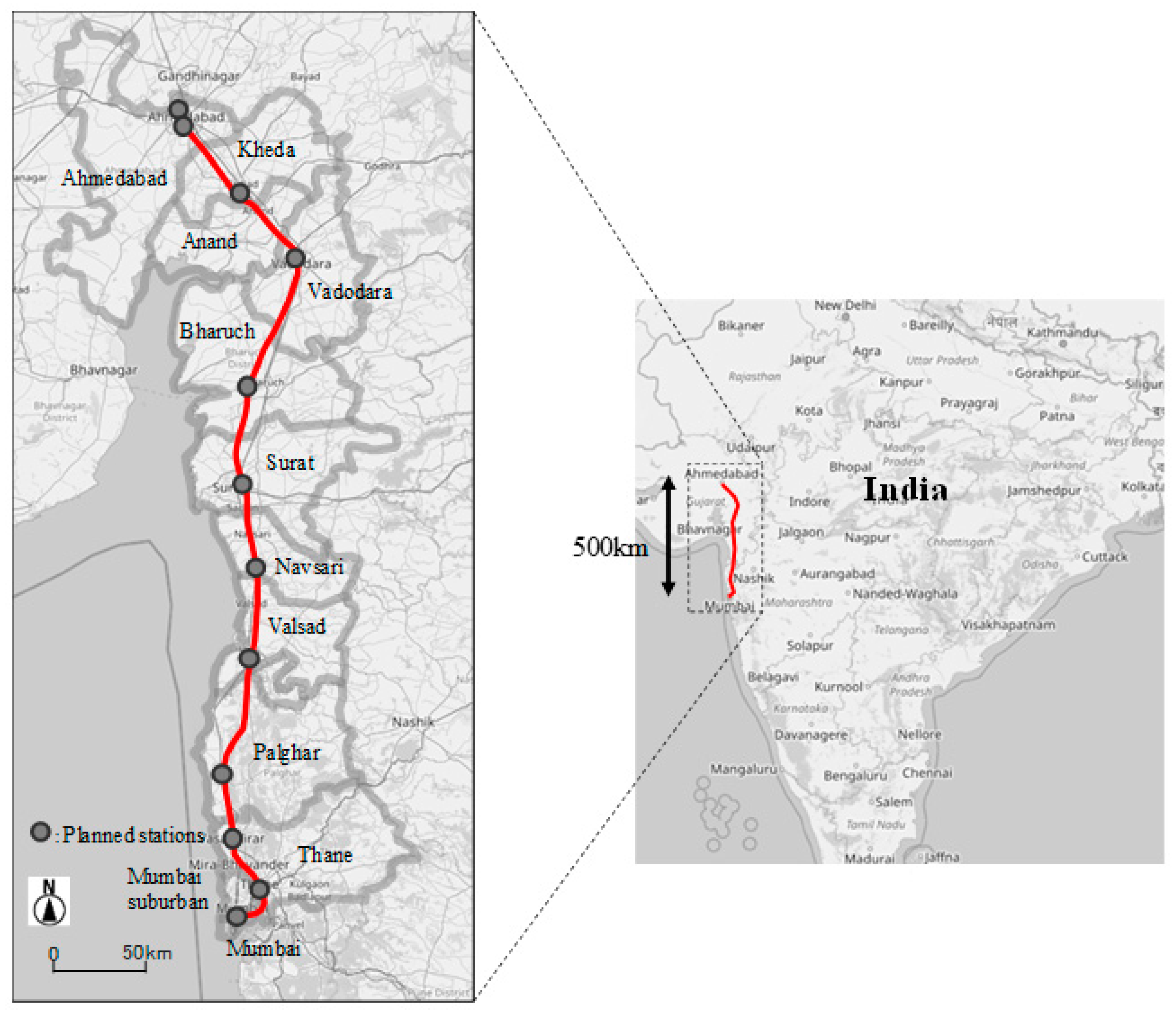
State	District	Population	Population Density (per km2)
Gujarat	Ahmedabad	7,214,225	890
	Kheda	2,299,885	582
	Anand	2,092,745	653
	Vadodara	4,165,626	552
	Bharuch	1,551,019	238
	Surat	6,081,322	1337
	Navsari	1,329,672	592
	Valsad	1,705,678	567
Maharashtra	Thane (including Palghar)	11,060,148	1157
	Mumbai (including suburban)	12,442,373	20,634
Total		49,942,693	1013 (average)

). This is much larger than the population of approximately 30 million [4] in the area along the Tokaido Shinkansen line in 1960 before the Shinkansen began operations.

From the perspective of an industrial structure, comparing the composition of employees by industry between the MAHSR corridor region in 2011 [5] (Figure 2a) and the Tokaido Shinkansen corridor region in 1960 [6] (Figure 2b), it can be seen that they have similar proportions for each industrial sector at the primary to tertiary levels. Additionally, comparing the flow of expenditure among industries and services between India in 2007 [7] and Japan in 1960 [8] by referring to the input–output (I/O) tables, similarities can be seen, e.g., in the proportion of expenditure flowing into manufacturing (Figure 3a,b).

Thus, what changes will be seen in the industrial interactions when the HSR is introduced in India and the passenger travel times between cities are reduced? In this study, the regional economic impacts as a part of the indirect benefits were analyzed by the model combining input–output (I/O) and spatial interaction, using the MAHSR corridor as a case study.

This approach allows the examination of interregional disparity that occurs with I/O interaction and distance impedance between the regions, and it is expected that this method will help the discussion for improvement in terms of economic development considering interregional equity in various emerging countries in the future.

2. Literature Review

The regional economic impacts of HSR have been discussed in a number of studies in recent years (e.g., Vickerman [9], Blanquart and Koning [10], and Chen et al. [11]). Chen and Silva [12] analyzed the long-term impact of Spain’s HSR network on employment and GDP using a panel structural equation modeling (SEM) formulation. Li et al. [13] investigated the redistribution of economic activities in the Yangtze River Delta region in China using the geographical network weighted regression model, and they showed that HSR drew an inflow into second-tier cities alongside the HSR for investment activities. Cheng et al. [14] examined changes in accessibility and provided evidence for the changes in specialization for the main cities and their hinterlands in China and Europe and then concluded that the processes of convergence and divergence vary by the stage of economic development. Vickerman [15] investigated the impact on the intermediate areas between major metropolitan areas along the network of northwest Europe and revealed that both levels of service and potential economic impacts were much less pronounced in these intermediate areas. The above discussions can be concluded in various ways depending on the social environment of each country and region including population distribution, urban structure, geographical conditions, and economic stage. Much discussion is still needed to establish analytical methods, and continued study and improvement are desirable.

The conventional cost–benefit analysis (CBA), which has been applied to many transportation projects including HSR, targets the direct benefits for users. However, in recent years, this concept has been reconsidered, and the need to capture wider economic impacts (WEI) as indirect benefits for non-users has been discussed. WEI is categorized into three types: induced investment, employment effects, and productivity impacts [16]. Among them, employment effects are related to changes in commuting behavior, mainly for intra-urban transit, while induced investment and productivity impacts are particularly related also to connectivity between metropolitan areas through intercity transportation such as HSR.

Regarding productivity impacts, Deng [17] summarized the various related literature estimating the contribution of transport infrastructure to productivity and economic growth. Rice et al. [18] found a robust relationship between productivity and proximity to economic mass. Chèze and Nègre [19] applied the UK agglomeration effects assessment method to the Bretagne Pays de Loire high-speed line in France and explored the possibility of assessing agglomeration and productivity gains. Thanh and Derrible [20] analyzed productivity and agglomeration changes and the wider economic impacts of an HSR project in Vietnam by measuring effective employment density. However, these studies did not take into account the I/O relationships among industries, i.e., the affinities and interactions among industries as expressed by input coefficients. We tried to combine the I/O interaction with productivity impact evaluation in this study.

In terms of ‘passenger or freight’, changes in the accessibility of passenger flow by HSR will assist in the development of a knowledge economy (Chen and Hall [21]) and regional innovation (Komikado et al. [22]) among multiple cities; in other words, it will bring communication effects related to the establishment of a new business or the promotion of existing business. These effects have different characteristics from those brought about by changes in freight transportation along with the construction of highways and roads. Yi and Kim [23] analyzed the spatial economic impacts of road and railway accessibility levels on manufacturing output in South Korea and revealed that there is not a substitutive but a complementary relationship between the two transportation modes. Related to the above, SCGE models have been applied to many transportation projects as the benefit analysis method at the microeconomic level (e.g., Tavasszy et al. [24], Koike et al. [25]); however, those are not necessarily versatile, because detailed statistical data, such as interregional input–output tables, are required.

As an alternative approach, the correlation between the industrial linkage and the actual changes in the number of employees in each industry, before and after the opening of the Nagano Shinkansen in Japan, was examined by Han, Hayashi, et al. [26], using a regression model that incorporates accessibility into the interdependence of inter–industrial transactions and consumption demand obtained from the I/O table. This is an extension of Nakamura, Hayashi, et al. [27] and Miyamoto et al. [28], which developed a model to predict industrial and commercial locations for a large metropolitan area in Japan, taking into account the economic distance between regions. This approach will be employed by the model in this study. In the abovementioned literature, the number of employees was applied as the explained variable, but since labor productivity actually differs from one industry to another, in this study, the production value was applied to represent productivity.

3. Methodology and Data

3.1. Model Setting

To represent the changes in the activity levels of industries and services induced by the shortening of travel time between cities following the opening of an HSR, we constructed an I/O–spatial interaction model by adding geospatial concepts to the I/O data. The modeling of geospatial distortions caused by the location of industries as an economic mass, which do not appear in general I/O data, was used to estimate the regional economic impacts caused by the distance impedance reduction associated with the opening of the MAHSR. The author developed the initial version of the I/O–spatial interaction model (Sugimori et al.) [29], and we applied an improved version in this study. The process of the model’s settings is described as follows.

In a case based on an ordinary I/O table, the relationship between the production value of each industry and aggregate demand for that industry, including both intermediate demand and final consumption demand, is as in Equation (1).

$$DI{N}^m={\displaystyle \sum }_k(A^{mk}\times PR{O}^k)$$

(1)

where $DI{N}^m$ is the demand for inter–industrial input from all industries to industry $m$; $PR{O}^k$ is the production value of industry $k$ (including final consumption demand as one of the industries); $A^{mk}$ is the input coefficient from industry $m$ to industry $k$. In this case, Equation (2) naturally holds.

$$PR{O}^m=DI{N}^m$$

(2)

Then, combining Equation (1) with the spatial distortion associated with distance decay, it can be expressed as Equations (3) and (4).

$$DI{N}_{ij}^{km}=A^{mk}\times PR{O}_i^k\times P{T}_{ij}^m$$

(3)

$$DI{N}_j^m={\displaystyle \sum }_i{\displaystyle \sum }_{k}DI{N}_{ij}^{km}$$

(4)

where $DI{N}_{ij}^{km}$ is the demand for inter–industrial input from industry $k$ in zone $i$ to industry $m$ in the surrounding zone $j$; $A^{mk}$ is the input coefficient from industry $m$ to industry $k$; $PR{O}_i^k$ is the production value of industry $k$ in zone $i$; $P{T}_{ij}^m$ is the probability of each industry in zone $i$ trading with industry $m$ in zone $j$. $P{T}_{ij}^m$ is derived from Equation (5).

$$P{T}_{ij}^m=\frac{EMP{L}_j^m\times {\left(G{C}_{ij}\right)}^{-{\lambda }^m}}{{{\displaystyle \sum }}_{j}EMP{L}_j^m\times {\left(G{C}_{ij}\right)}^{-{\lambda }^m}}$$

(5)

where $EMP{L}_j^m$ is the number of employees (as economic mass) of industry $m$ in zone $j$, $G{C}_{ij}$ is the generalized travel cost from zone $i$ to zone $j$, and ${\lambda }^m$ is the distance decay parameter of industry $m$. In this study, $G{C}_{ij}$ was calculated according to Equation (6) as the total monetary value, considering the time value and transportation modal share.

$$G{C}_{ij}={\displaystyle \sum }_n{s}_{ij}^n·\left(F_{ij}^n+\omega ·t_{ij}^n\right)$$

(6)

where $s_{ij}^n$, $F_{ij}^n$, and $t_{ij}^n$ are the modal share, transport fare and travel time, respectively, of the transportation mode $n$ from zone $i$ to zone $j$, and $\omega$ is the time value.

As described above, the spatial distribution of demand (expenditure) is expressed by considering the probability of trade between industries and services, determined by the distance-decayed economic mass (Figure 4). Accordingly, we define the main model as Equation (7), adding I/O–spatial interaction to the relationship in Equation (2).

$$\ln \left(PR{O}_j^m\right)={\alpha }^m\ln \left(DI{N}_j^m\right)+c^m$$

(7)

where ${\alpha }^m$ is the scale parameter, differing for each industry $m$; $c^m$ is a constant. This equation represents the agglomeration effects in a similar form to the Cobb–Douglas production function.

In reality, input coefficients change as time progresses. We recognize that the change is both due to performance progress in production and service and due to technological progress in transportation. Among them, in this model, the change of I/O volume between industries due to transportation technology progress is clearly shown. It was intended to be applied to the evaluation of various network improvements, such as the opening of HSR, which could not be expressed in an ordinary I/O model that discards spatial effects. I/O–spatial interaction model can be usually applied to any country and region which has I/O tables. It is an advantage of this method that we can well imagine the future changes in inter-industrial dependence due to technological progress in transportation. The Changes due to performance progress in production and service, and technical coefficients, are left for another study.

3.2. Data Used

3.2.1. Production Value and Input Coefficients

The production value and input coefficients of the MAHSR corridor region were estimated using data from the whole of India. Specifically, the regional economy in the MAHSR corridor was assumed closed internally, and the production value for the I/O table of the whole of India (2007) [7] was proportionally distributed according to the number of employees (2011) [5] in each industry and in each zone (based on the municipal unit of districts) along the MAHSR. In this case, the difference in production value between the MAHSR corridor region and the whole of India, resulting from the difference in the share of employees by industry, is regarded as the import or export value and deducted from the final consumption demand. Accordingly, the I/O table and the matrix of input coefficients $A^{mk}$ in the MAHSR corridor region were structured (

Table 2. Input coefficients $A^{mk}$ in the MAHSR corridor area.

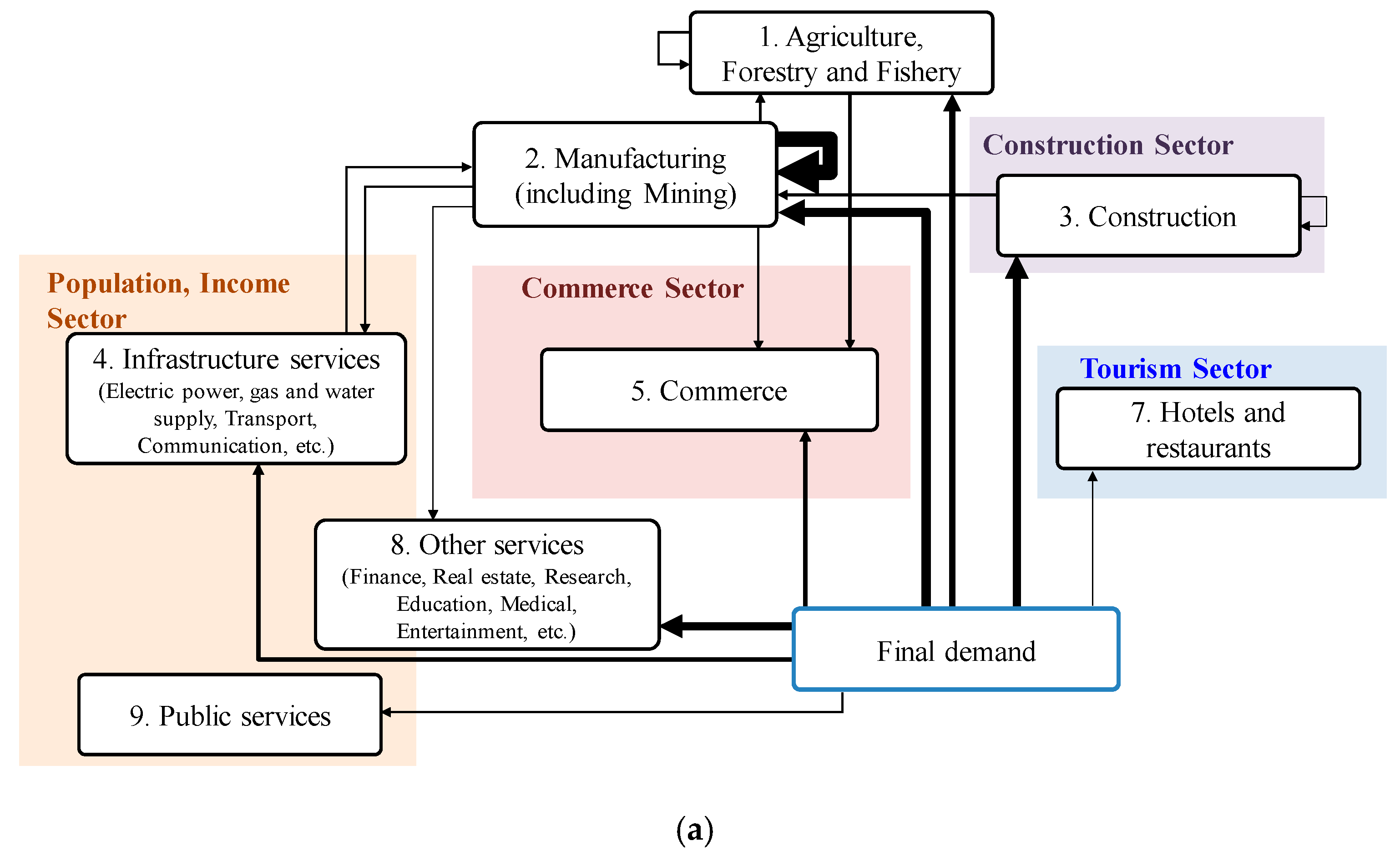
Industries and Services	Agriculture, Forestry and Fishery	Manufacturing (Including Mining)	Construction	Infrastructure Services	Commerce	Hotels and Restaurants	Other Services	Public Services	Final Consumption Demand
Agriculture, forestry, and fishery	0.19	0.07	0.03	0.01	0.00	0.25	0.00	0.00	0.10
Manufacturing (including mining)	0.06	0.47	0.30	0.27	0.06	0.20	0.05	0.00	0.36
Construction	0.01	0.01	0.12	0.01	0.00	0.02	0.02	0.00	0.14
Infrastructure services	0.03	0.08	0.06	0.08	0.06	0.05	0.04	0.00	0.10
Commerce	0.05	0.07	0.07	0.05	0.01	0.09	0.00	0.00	0.09
Hotels and restaurants	0.00	0.00	0.00	0.05	0.01	0.04	0.02	0.00	0.02
Other services	0.01	0.04	0.04	0.04	0.05	0.02	0.07	0.00	0.16
Public services	0.00	0.00	0.00	0.00	0.00	0.00	0.00	0.00	0.03
Value added	0.65	0.26	0.38	0.48	0.81	0.33	0.80	1.00	-
Total	1.00	1.00	1.00	1.00	1.00	1.00	1.00	1.00	1.00

).

The industries and services were categorized into eight types that were common to the various statistical data in India. The “Infrastructure services” consisted of electric power, gas, and water supply, transport, communication, etc., and the “Other services” consisted of finance, real estate, research, education, medical, entertainment, etc.

3.2.2. Generalized Travel Cost

In calculating the $G{C}_{ij}$ between each zone (between the central area of each zone) before and after the opening of the HSR, the transport mode share, fare, and travel time were set based on the results of the feasibility study of the MAHSR [30]. Additionally, the time value ω was calculated based on actual data in Japan. Specifically, the ω of MAHSR was set at seven rupees per min, which is one-sixth of the value of 40 yen per min in Japan [31], as the planned HSR fare between Mumbai and Ahmedabad is approximately 2300 rupees, which is about one-sixth of 14,500 yen for the Tokaido Shinkansen between Tokyo and Shin-Osaka in Japan [32]. Because both HSRs commonly take approximately two hours and have approximately 70% of the modal share [33], they are also expected to have users in almost the same income class. Note that the surrounding zone $j$ means zone $i$ itself also, and the fare and time between zone $i$ and itself were set at half of the average fare and time between zone $i$ and neighboring zones. The generalized travel cost $G{C}_{ij}$ set between the zones without the MAHSR is shown in

Table 3. Generalized travel cost $G{C}_{ij}$ (INR) set between the zones in the MAHSR corridor area (without MAHSR) (INR).

	Ahmedabad	Kheda	Anand	Vadodara	Bharuch	Surat	Navsari	Valsad	Thane	Mumbai
Ahmedabad	249	592	958	1252	1996	2688	2944	3232	4831	5573
Kheda	592	223	419	792	1572	2232	2526	2820	3466	5197
Anand	958	419	193	439	1227	1853	2156	2459	3204	5041
Vadodara	1252	792	439	323	914	1550	1853	2166	2920	4805
Bharuch	1996	1572	1227	914	387	712	1035	1348	2428	3732
Surat	2688	2232	1853	1550	712	267	419	722	1820	3064
Navsari	2944	2526	2156	1853	1035	419	186	409	1506	2559
Valsad	3232	2820	2459	2166	1348	722	409	366	1146	2232
Thane	4831	3466	3204	2920	2428	1820	1506	1146	545	1136
Mumbai	5573	5197	5041	4805	3732	3064	2559	2232	1136	551

.

3.2.3. Distance Decay Parameter

The distance decay parameter ${\lambda }^m$ may be set at 1.000 uniformly for all industries practically in the simplest way (e.g., Gutierrez [34] and Venables et al. [35]); however, in reality, the distance impedance is expected to be individually different for each industry $m$, so the distance decay parameter by industry from Graham et al. [36] and the Department for Transport [37] were applied (Case 1). Though these values were estimated from commuting demand within the UK metropolitan area, we applied them because they can be utilized in terms of distinguishing relative differences in the distance decay by industry. For examining sensitivity by various distance decay parameters ${\lambda }^m$, Case 2 (foot-loose case) and Case 3 (foot-tight case) were added as shown in

Table 4. Distance decay parameter $\lambda$ set for each industry.

	Case 1	Case 2	Case 3
Agriculture, forestry, and fishery	1.655	1.000	1.800
Manufacturing (including mining)	1.097	1.000	1.800
Construction	1.562	1.000	1.800
Infrastructure services	1.818	1.000	1.800
Commerce	1.818	1.000	1.800
Hotels and restaurants	1.818	1.000	1.800
Other services	1.746	1.000	1.800
Public services	1.655	1.000	1.800

.

4. Estimation and Results

4.1. Estimated Parameter

The results of the parameter estimation using the regression model in Equation (7) are shown in

Table 5. Estimated parameters (Case 1).

	$\mathit{\alpha }$	$\mathit{c}$	R2
Agriculture, forestry, and fishery	0.988	0.144	0.53
	(3.34)	(0.04)
Manufacturing (including mining)	0.959	0.634	0.99
	(35.01)	(1.63)
Construction	0.976	0.290	0.97
	(16.71)	(0.39)
Infrastructure services	1.031	−0.536	0.94
	(11.42)	(−0.46)
Commerce	0.957	0.548	0.97
	(15.69)	(0.71)
Hotels and restaurants	1.077	−1.191	0.92
	(10.48)	(−1.04)
Other services	0.971	0.349	0.95
	(12.85)	(0.35)
Public services	1.186	−2.611	0.91
	(9.29)	(−1.90)

(The bracketed values are t-values).

as a representative example for Case 1. It is inferred that industries with a relatively high-scale parameter α value (infrastructure services, hotels, and restaurants, public services, etc.) may multiplicatively gain economic impacts by reacting to the increase in demand for input.

4.2. Regional Economic Impacts Evaluation

Using the scale parameter $\alpha$ obtained above, the economic impacts brought to the MAHSR corridor region were evaluated. Specifically, on the right-hand side of Equation (5), which determines the probability of trade $P{T}_{ij}^m$, substituting the generalized travel cost $G{C}_{ij}$ without the MAHSR in the denominator, and $G{C}_{ij}$ with MAHSR (

Table 6. Generalized travel cost $G{C}_{ij}$ (INR) set between the zones in the MAHSR corridor area (with MAHSR).

	Ahmedabad	Kheda	Anand	Vadodara	Bharuch	Surat	Navsari	Valsad	Thane	Mumbai
Ahmedabad	249	498	955	1252	1996	2564	2818	2994	3919	4307
Kheda	498	223	377	792	1572	2232	2526	2753	3466	4240
Anand	955	377	193	397	1227	1853	2156	2459	3204	4241
Vadodara	1252	792	397	323	885	1550	1853	2166	2920	3897
Bharuch	1996	1572	1227	885	387	682	1035	1348	2428	3530
Surat	2564	2232	1853	1550	682	267	419	722	1820	2903
Navsari	2818	2526	2156	1853	1035	419	186	409	1506	2421
Valsad	2994	2753	2459	2166	1348	722	409	366	1116	2216
Thane	3919	3466	3204	2920	2428	1820	1506	1116	545	1136
Mumbai	4307	4240	4241	3897	3530	2903	2421	2216	1136	551

) in the numerator, it was expressed that newly induced demand will arise due to the reduction in travel time. In addition, by using Equation (7), the increase in production value $PR{O}_j^m$ in reaction to increased demand for input $DI{N}_j^m$ was estimated.

Additionally, substituting the following Equation (8) into Equation (5), Equation (9) is obtained.

$$EMP{L}_j^m=\frac{PR{O}_j^m}{L{P}^m}$$

(8)

$$P{T}_{ij}^m=\frac{PR{O}_j^m\times {\left(G{C}_{ij}\right)}^{-{\lambda }^m}}{{{\displaystyle \sum }}_{j}PR{O}_j^m\times {\left(G{C}_{ij}\right)}^{-{\lambda }^m}}$$

(9)

where $L{P}^m$ is the labor productivity of industry $m$. In this case, when substituting the production value $PR{O}_j^m$ estimated by Equation (7) into Equation (9), $P{T}_{ij}^m$ is renewed. Accordingly, $DI{N}_j^m$ obtained by Equations (3) and (4) is also renewed, and to be corrected back by iterative calculation. In this calculation, $DIN$ by industry is proportionally adjusted while $DIN$ by zone is fixed, because the supply of land and labor as production factors tend to be geographically invariant.

Table 7. Annual GRP increases (billion INR) by industry and by zone (Case 1).

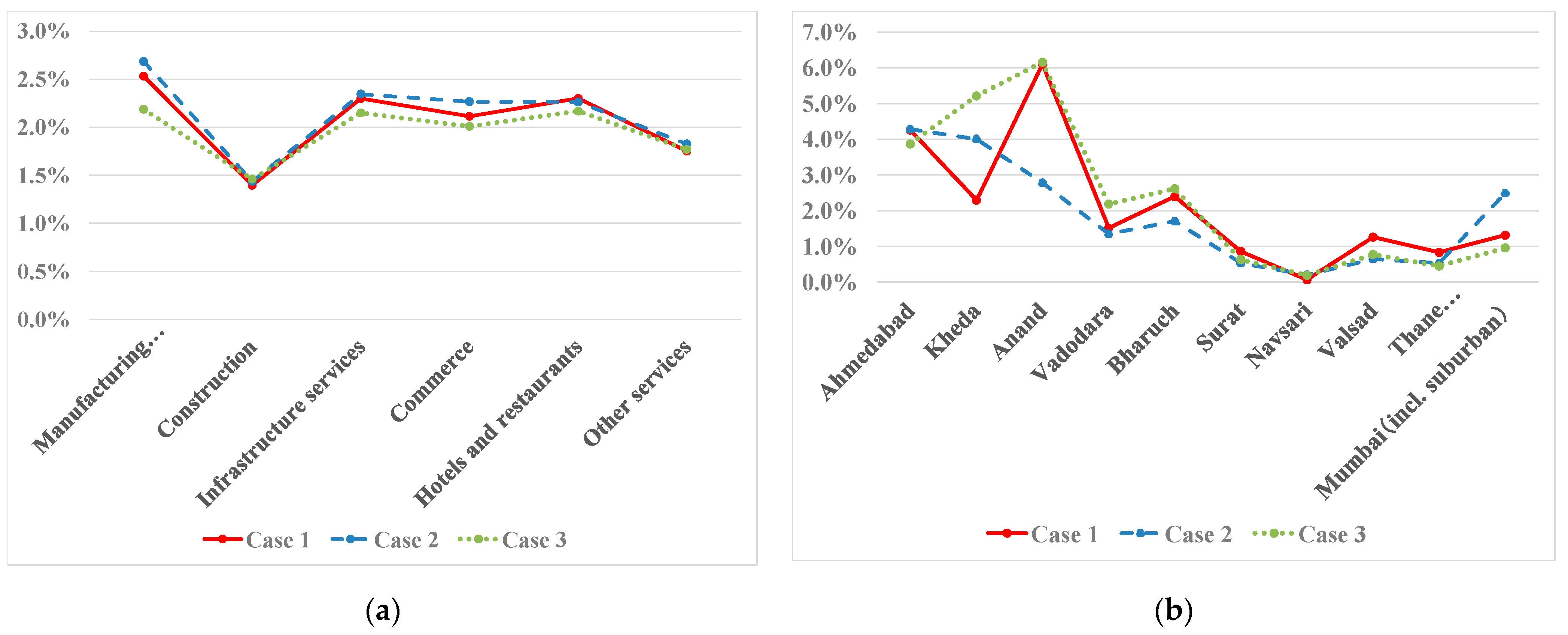
	Manufacturing (Including Mining)	Construction	Infrastructure Services	Commerce	Hotels and Restaurants	Other Services	Total
Ahmedabad	4.6	1.7	2.4	4.4	0.3	4.3	17.6
Kheda	4.3	−0.4	−0.2	−1.0	−0.2	−0.7	1.9
Anand	0.6	0.4	1.0	1.5	0.3	1.9	5.6
Vadodara	3.3	0.0	−0.3	0.3	−0.2	−0.5	2.7
Bharuch	0.0	0.1	0.5	0.0	0.0	0.6	1.3
Surat	1.6	0.2	0.4	1.3	0.1	0.6	4.1
Navsari	0.4	0.0	−0.1	−0.1	−0.1	−0.1	0.1
Valsad	0.4	0.1	0.0	0.3	0.0	0.3	1.0
Thane	0.5	0.5	1.1	1.2	0.2	1.7	5.2
Mumbai	3.3	0.2	1.9	1.4	0.5	1.3	8.6
Total	19.1	2.6	6.8	9.3	0.8	9.4	48.1

shows the annual GRP increase by industry and by zone with MAHSR (as a representative example for Case 1), which was obtained by multiplying the estimated production value by the input coefficients $A$ of “Value added” in Table 2. In this estimation, “Agriculture, forestry, and fishery” and “Public services” were excluded because the relationship between the location conditions of those industries and intercity passenger flow was considered trivial.

Similarly, Figure 5a,b shows the increasing rate of annual GRP by industry and by zone, respectively. Though there was some variation in the results for each case according to the differences in the distance decay parameter $\lambda$, commonly in all cases, it can be seen that the increase rate of annual GRP for each zone in Gujarat State, including Ahmedabad, was relatively high, being newly connected to Mumbai. Moreover, these results suggest that smaller- and medium-sized intermediate cities can also gain economic benefits to a certain extent. The increase rate of annual GRP averaged in the MAHSR corridor region was 1.6%~1.8% (

Table 8. Increasing rate of annual GRP averaged in the MAHSR corridor region.

Case 1	Case 2	Case 3
1.8%	1.8%	1.6%

).

In Table 7 and Figure 5, the GRP effects of network improvement by high-speed rail are not uniform across industries and regions, i.e., the possibility of interregional disparity is quantitatively expressed. Figure 5a shows that Case 2 (foot-loose case) tends to produce greater interaction effects than Case 3 (foot-tight case) in all industries and services. Figure 5b shows that in Case 2, Mumbai and Ahmedabad (especially Mumbai) with large economic mass have an advantage over smaller cities, which means the so-called straw effect. In other words, while the reduction of distance impedance by HSR installation may promote regional economic development, it may also widen the economic gap among cities in the HSR corridor area. In order to maintain the economy of each city from being absorbed into that of the larger metropolitan areas, it will be important to develop a unique industrial structure, which helps to either preserve or enhance $PT$ in Equation (3). As an example of the Tokaido Shinkansen corridor in Japan, the industrial base, especially manufacturing, which is well anchored in Nagoya City, was not swallowed up by Tokyo (Hayashi et al. [38]).

The abovementioned annual GRP increases are expressed as the difference between ‘without the MAHSR’ economic sizes of the MAHSR corridor at a given point in time (2007 in this study) versus the assumed ‘with the MAHSR’ transportation network, along with its geographic distribution. This was shown as the additional economic scale that could be obtained indirectly, apart from the macroeconomic growth of the region as a whole.

5. Conclusions

This study evaluated the regional economic impacts as a part of the indirect benefits brought by the Mumbai–Ahmedabad High-Speed Rail (MAHSR), which is currently under construction. In order to estimate the impacts, we modeled the I/O–spatial interaction by combining the inter–industrial transaction shown on the I/O table with the geospatial distance decay of economic mass through passenger transportation.

The results showed the economic impacts on each zone and each industry along the MAHSR corridor as a relative distribution. In addition, the increase rate of annual GRP averaged among all industries and zones was estimated as 1.6%~1.8% (variation by distance decay parameter $\lambda$ set in this study). In this estimation, it was assumed that the production value of each industry in each city would increase by completely accepting the newly induced demand coming in. However, if a scenario in which industrial location and labor flow freely among cities is assumed, industrial concentration in larger metropolitan areas, as well as interregional disparity, may occur, which means a straw effect. In order to maintain the economy of each city from being absorbed into that of the larger metropolitan areas, it will be important to develop a unique industrial structure.

As described above, the unique feature of this approach is that it is possible to evaluate the geographic distributions and interregional disparity of economic impacts by combining the industrial I/O relationships with the changes in passenger accessibility associated with a large-scale transportation project such as HSR. In addition, this method can be applied to various countries and regions where detailed I/O statistical data, such as interregional I/O tables, are difficult to obtain, as well as various transportation project evaluations taking into account interregional equity.

For future work, the statistical data used should be updated, and the model should be applied to multiple cases in other HSR corridor regions in India and abroad and validated based on empirical evidence. In addition, it will be possible to estimate a wide range of effects of HSR by combining impacts on the regional economy with QOL improvement as impacts on personal well-being, which can be estimated by the ‘QOL accessibility method’ (Hayashi et al. [39]).

References

- National High Speed Rail Corporation Limited, MAHSR Operational Plan. Available online: https://www.nhsrcl.in/en/project/mahsr-project-operational-planss (accessed on 10 July 2022).
- OpenStreetMap. Available online: https://www.openstreetmap.org/#map=6/16.286/77.124 (accessed on 10 July 2022).
- Ministry of Home Affairs, Government of India, Census Tables, D-01. Available online: https://censusindia.gov.in/census.website/data/census-tables (accessed on 10 July 2022).
- Statistics Bureau of Japan, 1960 Population Census, Population, Area and Population Density for Shi, Ku, Machi and Mura: 1960. Available online: https://www.e-stat.go.jp/en/stat-search/files?page=1&layout=datalist&toukei=00200521&tstat=000001036867&cycle=0&tclass1=000001037497&tclass2val=0 (accessed on 10 July 2022).
- Ministry of Home Affairs, Government of India, Census Tables, B-04. Available online: https://censusindia.gov.in/census.website/data/census-tables (accessed on 10 July 2022).
- Statistics Bureau of Japan, 1960 Population Census, Industry (Minor Group) of Employed Persons 15 Years Old and Over by Employment Status and Sex, for All Japan, Prefectures and 6 Major Cities. Available online: https://www.e-stat.go.jp/en/stat-search/files?page=1&layout=datalist&toukei=00200521&tstat=000001036867&cycle=0&tclass1=000001038048&tclass2val=0 (accessed on 10 July 2022).
- Central statistics office, Ministry of statistics and programme implementation, Government of India, Input-Output table 2007–08, 2012. Available online: http://164.100.161.63/publication/input-output-transactions-table-2007-08 (accessed on 10 July 2022).
- Ministry of Internal Affairs and Communications, Input-Output Table, 1960. Available online: https://www.soumu.go.jp/toukei_toukatsu/data/io/960index.htm (accessed on 10 July 2022). (In Japanese)
- Vickerman, R. Can high-speed rail have a transformative effect on the economy? Transp. Policy 2018, 62, 31–37. [Google Scholar] [CrossRef]
- Blanquart, C.; Koning, M. The local economic impacts of high-speed railways theories and facts. Eur. Transp. Res. Rev. 2017, 9, 1–14. [Google Scholar] [CrossRef]
- Chen, C.; Loukaitou-Sideris, A.; De Ureña, J.M.; Vickerman, R. Spatial short and long-term implications and planning challenges of high-speed rail: A literature review framework for the special issue. Eur. Plan. Stud. 2019, 27, 415–433. [Google Scholar] [CrossRef]
- Chen, G.; Silva, J.A. Estimating the provincial economic impacts of high-speed rail in Spain: An application of structural equation modelling. Procd. Soc. Behv. 2014, 111, 157–165. [Google Scholar] [CrossRef]
- Li, X.; Huang, B.; Li, R.; Zhang, Y. Exploring the impact of high speed railways on the spatial redistribution of economic activities-Yangtze River Delta urban agglomeration as a case study. J. Transp. Geogr. 2016, 57, 194–206. [Google Scholar] [CrossRef]
- Cheng, Y.; Loo, B.P.Y.; Vickerman, R. High-speed rail networks, economic integration and regional specialisation in China and Europe. Travel Behav. Soc. 2015, 2, 1–14. [Google Scholar] [CrossRef]
- Vickerman, R. High-speed rail and regional development: The case of intermediate stations. J. Transp. Geogr. 2015, 42, 157–165. [Google Scholar] [CrossRef]
- Department for Transport, Transport Analysis Guidance (TAG) Unit A2-1 Wider Economic Impacts Appraisal, May 2019. Available online: https://www.gov.uk/government/publications/tag-unit-a2-1-wider-economic-impacts (accessed on 10 July 2022).
- Deng, T. Impacts of transport infrastructure on productivity and economic growth: Recent advances and research challenges. Transp. Rev. 2013, 33, 686–699. [Google Scholar] [CrossRef]
- Rice, P.; Venables, A.J.; Patacchini, E. Spatial determinants of productivity: Analysis for the regions of Great Britain. Reg. Sci. Urban Econ. 2006, 36, 727–752. [Google Scholar] [CrossRef]
- Chèze, C.; Nègre, R. Wider economic impacts of high-speed rail: Example of agglomeration benefits assessment on Bretagne Pays de Loire high speed rail project. Transport. Res. Procedia 2017, 25, 5307–5324. [Google Scholar] [CrossRef]
- Thanh, T.T.M.; Derrible, S. Assessing the wider economic impacts of transport infrastructure investment with an illustrative application to the North-South High-Speed Railway Project in Viet Nam. In Frontiers in High-Speed Rail Development; Hayashi, Y., Rothengatter, W., Seetha Ram, K.E., Eds.; Asian Development Bank Institute: Tokyo, Japan, 2021; pp. 181–196. [Google Scholar]
- Chen, C.; Hall, P. The wider spatial-economic impacts of high-speed trains: A comparative case study of Manchester and Lille sub-regions. J. Transp. Geogr. 2012, 24, 89–110. [Google Scholar] [CrossRef]
- Komikado, H.; Morikawa, S.; Bhatt, A.; Kato, H. High-speed rail, inter-regional accessibility, and regional innovation: Evidence from Japan. Technol. Forecast. Soc. 2021, 167, 120697. [Google Scholar] [CrossRef]
- Yi, Y.; Kim, E. Spatial economic impact of road and railroad accessibility on manufacturing output: Inter-modal relationship between road and railroad. J. Transp. Geogr. 2018, 66, 144–153. [Google Scholar] [CrossRef]
- Tavasszy, L.A.; Thissen, M.J.P.M.; Oosterhaven, J. Challenges in the application of spatial computable general equilibrium models for transport appraisal. Res. Transp. Econ. 2011, 31, 12–18. [Google Scholar] [CrossRef]
- Koike, A.; Ishikura, T.; Miyashita, M.; Tsuchiya, K. Spatial Economic Analysis for Intercity Transport Policies. In Intercity Transport and Climate Change; Hayashi, Y., Morichi, S., Oum, T., Rothengatter, W., Eds.; Springer: Berlin/Heidelberg, Germany, 2014; pp. 177–213. [Google Scholar]
- Han, J.; Hayashi, Y.; Jia, P.; Yuan, Q. Economic Effect of High-Speed Rail: Empirical analysis of Shinkansen’s impact on industrial location. J. Transp. Eng. 2012, 138, 1551–1557. [Google Scholar] [CrossRef]
- Nakamura, H.; Hayashi, Y.; Miyamoto, K. A land use-transport model for metropolitan areas. Pap. Reg. Sci. Assoc. 1983, 51, 43–63. [Google Scholar] [CrossRef]
- Miyamoto, K.; Nakamura, H.; Hayashi, Y. Industrial location model in metropolitan areas. Proc. Jpn. Soc. Civ. Eng. 1983, 339, 155–165. (In Japanese) [Google Scholar] [CrossRef]
- Sugimori, S.; Hayashi, Y.; Takeshita, H. Empirical analysis on industrial sectors for quality of life improvement along high-speed rail corridors. In Frontiers in High-Speed Rail Development, 1st ed.; Hayashi, Y., Rothengatter, W., Seetha Ram, K.E., Eds.; Asian Development Bank Institute: Tokyo, Japan, 2021; pp. 218–228. [Google Scholar]
- Japan International Cooperation Agency (JICA), Ministry of Railways, Republic of India (MOR), Joint Feasibility Study for Mumbai-Ahmedabad High Speed Railway Corridor, Final Report, July 2015. Available online: https://www.nhsrcl.in/en/project/feasibility-study-report (accessed on 10 July 2022).
- Railway Bureau, Ministry of Land, Infrastructure, Transport and Tourism. Appraisal Method Manual for Railway Projects, 2012. Available online: https://www.mlit.go.jp/tetudo/tetudo_fr1_000040.html (accessed on 10 July 2022). (In Japanese)
- Central Japan Railway Company, Fares and Surcharges. Available online: https://global.jr-central.co.jp/en/info/fare/ (accessed on 10 July 2022).
- Ministry of Land, Infrastructure, Transport and Tourism, 2015 Inter-Regional Travel Survey in Japan. Available online: https://www.mlit.go.jp/sogoseisaku/soukou/sogoseisaku_soukou_fr_000016.html (accessed on 10 July 2022).
- Gutiérrez, J. Location, economic potential and daily accessibility: An analysis of the accessibility impact of the high-speed line Madrid-Barcelona-French border. J. Transp. Geogr. 2001, 9, 229–242. [Google Scholar] [CrossRef]
- Venables, A.J.; Laird, J.; Overman, H. Transport Investment and Economic Performance: Implications for Project Appraisal. 2014. Available online: https://assets.publishing.service.gov.uk/government/uploads/system/uploads/attachment_data/file/386126/TIEP_Report.pdf (accessed on 10 July 2022).
- Graham, D.J.; Gibbons, S.; Martin, R. Transport Investment and the Distance Decay of Agglomeration Benefits. 2009. Available online: https://www.researchgate.net/publication/228793866_Transport_investment_and_the_distance_decay_of_agglomeration_benefits (accessed on 10 July 2022).
- Department for Transport, Transport Analysis Guidance (TAG) Unit A2-4 Productivity Impacts, May 2020. Available online: https://www.gov.uk/government/publications/tag-unit-a2-4-productivity-impacts (accessed on 10 July 2022).
- Hayashi, Y.; Mimuro, A.; Han, J.; Kato, H. The Shinkansen and its impacts. In High-Speed Rail and Sustainability; Henriquez, B.L.P., Deakin, E., Eds.; Routledge: New York, NY, USA, 2017; pp. 34–49. [Google Scholar]
- Hayashi, Y.; Morita, H.; Takeshita, H.; Kachi, N.; Kato, H. (Eds.) Mainstreaming Quality of Life in Evaluation of Transport and Spatial Planning, 1st ed.; Akashi Shoten: Tokyo, Japan, 2021; 380p. (In Japanese) [Google Scholar]