Abstract
The concept of hydraulic impedance is widely used for periodic or oscillating flow scenarios in applied hydraulic transients. This paper proposes an equivalent circuit-based discrete hydraulic impedance model for the hydraulic system of the power station. The equivalent hydraulic circuit is established by an analogy between the water hammer wave propagation in pressurized pipes and the electromagnetic wave propagation in conductors. The discrete hydraulic impedance at a given location is obtained by calculating the total specific impedance of the series and parallel circuits from one end to the other. In addition, the numerical solution process to obtain the natural frequencies of the system via the proposed model is designed in detail. Furthermore, oscillation characteristics of the pipelines in the hydropower station are investigated. The variation trends of the decay coefficients of different orders of oscillation of the system and the influence of turbine impedance on the oscillation frequencies are discussed, respectively.
1. Introduction
Transient analyses of hydropower systems often are carried out via numerical simulation schemes based on time and space discretization, such as the method of characteristics (MOC) [1], the finite difference/volume method [2,3], and the transfer function/differential equations [4,5]. The basic idea of these time domain numerical schemes is to transform continuous systems into discrete systems [6], thus reducing the degree of freedom in the system model and calculating the time evolutions of system states with satisfactory computational cost and numerical precision. However, most time domain numerical schemes are under the constraint of the Courant condition [7], where the Courant number is required to be close to one to restrain the numerical dissipation. The strong constraint will bring a substantial computational burden to the complex high-order systems. In addition, due to the nonlinearities, such as the dissipative terms and the uncertain parameters in these models [8], it is difficult to be implemented in the system stability analysis. Therefore, frequency domain methods, as another alternative, were extensively explored for stability analysis [2,9].
The conventional frequency domain schemes, e.g., the hydraulic impedance method [10,11,12,13,14] and the transfer matrix method [2], are widely used in applied hydraulic transients. The hydraulic impedance, defined as the complex head deviation divided by the complex flow rate deviation, is always formulated as a function of the complex frequency s. The relationship between the piezometric head and the discharge at an arbitrary longitudinal position along a pipe or a channel can be explicitly described with the model. This method shows potential for the leakage calibration [15], blockage detection [16,17], and the resonance analysis [18]. Suo and Wylie [8] obtained the response of a steady oscillatory flow with the linearized Saint-Venant equations of a pressurized pipe. Kim [11] formulated an impedance matrix model for complicated pipe networks and discussed the superiority of the impulse response method over other time domain schemes. In addition, he also discussed the dynamic matrix computation method [12] and incorporated the genetic algorithm into the address-oriented impedance matrix for the generic calibration of the system parameters of the pipe networks with complex topology [13]. Zhou et al. [14] investigated the self-excited hydraulic and mechanical vibration characteristics of the pumped storage power station based on the hydraulic impedance method. The free and forced oscillation responses were obtained and analyzed through this approach. Yang [9] systematically revealed the mathematical expressions of the hydraulic impedances of different components in the hydropower station, including the hydraulic turbine, the pressurized pipe, and the reservoir. Moreover, the stability of the hydropower station under different operating conditions is investigated with the hydraulic impedance method.
The traditional continuous hydraulic impedance can handle complex frequency domain modeling of simple pipe networks, such as pipes in series, pipe networks with single branches, and single loops. However, it cannot address the modeling of high-dimensional hydraulic networks with multi-loops very well. To fully take advantage of the well-developed circuit theory, the methodology of the complex frequency domain equivalent circuit-based hydraulic impedance model is inspired to calculate the specific impedance of any given location along the complicated pipeline by considering the pipe network as a discrete system. The basic idea of this resolution, inspired by an analogy between the hydraulic circuit and the electrical conductor, was first mentioned by Paynter [19] and Jaeger [20]. Souza Jr. [21] performed the numerical analysis of hydraulic transients in a hydropower plant using this methodology. Dr. Nicolet [22] extended the equivalent circuit model (ECM) to the mathematical modeling of different hydraulic facilities and validated its effectiveness in the simulation of hydraulic transients in engineering practice. Over the past few years, Zhao et al. [23] applied ECM to the dynamic analysis of operating condition conversion processes in a pumped storage plant. Zheng et al. [24] expanded the ECM to describe hydraulic transients of a hydraulic system with pipe and open channel flows and achieved satisfactory simulation precision. To the best of the authors’ knowledge, most of the existing literature about this approach only focused on its privilege in the time domain numerical simulation [19,20,21,22,23,24]. Seldom was the equivalent circuit-based complex frequency-domain analysis reported. Although Nicolet [25] discussed the application of the frequency domain ECM to obtain the frequency responses in the reservoir–pipe–valve system, the system discussed is too simple to fully reflect the complex frequency domain description capability of the ECM. Therefore, it is necessary to further explore the features of the complex frequency domain ECM in more complicated hydraulic systems.
This paper proposes an equivalent circuit-based discrete hydraulic impedance model for the power station system. The equivalent hydraulic circuit is established by an analogy between the water hammer wave propagation in pressurized pipes and the electromagnetic wave propagation in conductors. The discrete hydraulic impedance at any discrete node is obtained by calculating the total specific impedance from one boundary side to the other according to the circuit theory. Subsequently, the detailed procedure of the free oscillation response analysis of the system via the proposed discrete impedance model is introduced. According to the oscillation analysis process, the variation trends of the decay coefficients of different orders of oscillation for the diversion and tailrace pipelines are discussed. Furthermore, the influence of turbine impedance on the decay coefficients and the frequencies corresponding to different orders of oscillation are investigated, respectively.
The rest of this paper is organized as follows: First, the methodology of the equivalent circuit-based hydraulic impedance for different hydraulic components, such as the pressurized pipe and the hydraulic turbine is introduced in Section 2. In Section 3, the overall equivalent circuit topology for the hydraulic system of the studied hydropower station is presented, and the detailed numerical solution process of the free oscillation response is illustrated. Then, numerical simulation results of the free oscillation responses for the hydropower station system are presented, and the variation trends of the system oscillation responses are systematically analyzed in Section 4. Eventually, the conclusions are given in Section 5.
2. Methodology of the Discrete Hydraulic Impedance
2.1. Equivalent Circuit of a Pressurized Pipe
The continuity equation and the momentum equation are the basic physical rules to describe the movement of fluids, such as wave propagation [26,27] and water delivery [28]. To mathematically characterize the dynamic behavior of fluid transients in a pressurized pipe, the well-known one-dimensional Saint-Venant equations [2,9] are stated in Equation (1),
where the subscript i denotes the pipe number. Hydraulic phenomena are characterized by a high wave speed a and a relatively much lower flow velocity v, so the convective terms related to the transport characteristic can be neglected with respect to the propagative terms in Equation (1). Thus, when the piezometric head H and discharge Q are taken as state variables, the Saint-Venant equation in Equation (1) has the same formulation as the telegraphist’s equations [22,25]. As expressed in Equation (2),
where the values of the equivalent RLC parameters per unit length are stated in Equation (3),
The equivalent resistance Rei, the equivalent inductance Lei, and the equivalent capacitance Cei are related to the head losses through the pipe, the inertia effect of the water, and the storage effect caused by pressure variation, respectively. These three different circuit components are essential to precisely model a pressurized pipe. The equivalent circuit of a pressurized pipe containing n segments is displayed in Figure 1. The hydraulic transients along a pipeline are characterized as a discrete RLC circuit in which the state variables, i.e., the piezometric head and the discharge, can be obtained only for given locations x and given times t, according to the sizes of the time step dt and the spatial mesh dx.
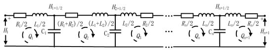
Figure 1.
The equivalent circuit of a pressurized pipe.
Apart from the time domain differential equations for numerical simulation [19,20,21,22,23,24,25], the ECM can also be used to investigate the complex frequency-related features of the hydraulic system, such as the transfer matrix and the hydraulic impedance. The transfer matrix is often used to calculate the forced oscillation responses of the system, while the hydraulic impedance is more suitable for free oscillation analysis. In this study, we focus on the free oscillation analysis. If a pipe is modeled by n T-shape equivalent circuit segments, the equivalent impedance is calculated recursively from one end of the pipe according to the circuit theory. The equivalent impedance of the ith loop can be obtained with Equation (4),
where, , and . The positive directions of the piezometric head and discharge are set as directions shown in Figure 1. When the impedance is calculated from the upstream side to the downstream side, the directions of the piezometric head and discharge follow the preset positive direction, otherwise, the direction of discharge follows the negative direction. It should be emphasized that Equation (4) works when discharges follow the directions marked in Figure 1. Otherwise, the hydraulic impedance when the discharges are in the opposite direction, where is the impedance calculated with Equation (4).
The proposed complex frequency domain ECM transforms the piping system into a spatial discretization approximation of the continuous system, while the traditional impedance method computes the impedance of a certain location directly through the analytical solution. The pipe is divided into several pipe segments in the ECM, which brings inevitable numerical error led by spatial discretization. However, the well-developed circuit theory enables the ECM to be applied to systems with complex hydraulic layouts. For complete frictionless systems, the system impedances can be calculated at one end for a given range of frequencies and identify which satisfies the known boundary conditions. For dissipative systems, the problem then becomes searching for the complex frequencies satisfying all the hydraulic boundary conditions. It usually leads to an iterative numerical solving process searching for the minimum of a predefined objective function.
2.2. Typical Hydraulic Boundary Treatments
The treatment of different boundaries is also important for hydraulic system modeling [29].
2.2.1. Hydraulic Turbine
The hydraulic turbine is usually considered one of the most complicated hydraulic boundaries in the transient analysis of the hydropower station system. According to the theory proposed by Wylie and Streeter [30], the hydraulic impedance of the hydraulic turbine can be reflected by Equation (5),
where the impedance is highly related to the characteristic curves of the hydraulic turbine. n and D1 are the rotational speed and runner’s diameter, respectively. n11 and Q11 denote the unit rotational speed and unit discharge, respectively.
Suppose that k1 = Q11/n11 and , it is found that only if k1 < k2, will the hydraulic impedance of the turbine ZT be negative, otherwise the value of ZT is positive. Seen from Figure 2, the slope of Q11/n11 is always positive and the slope of is negative, which means that the turbine impedance ZT > 0 when the power station is in steady turbine operation.
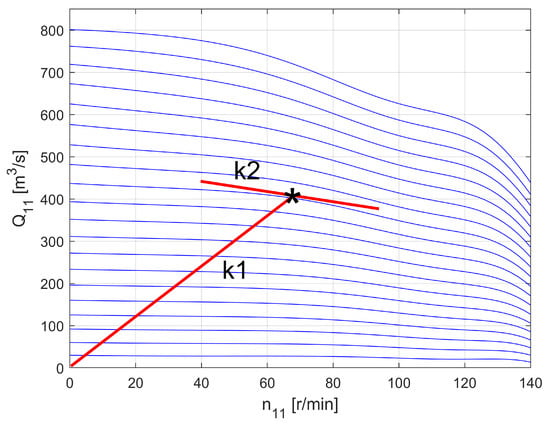
Figure 2.
The discharge characteristic curve of a hydraulic turbine.
2.2.2. Reservoir
For most scenarios of applied hydraulic transients, the water level of a reservoir is often assumed to keep constant during the whole process of interest regardless of the possible variation in discharges, i.e., the piezometric head variation . Therefore, the reservoir boundary can be treated as an open end, i.e., the impedance .
3. Oscillation Analysis of the Hydraulic System of a Hydropower Station
3.1. Introduction to the System Plant
A hydropower station system, firstly introduced in [9], is taken as the system plant in this study. The structural schematic of the system is depicted in Figure 3.
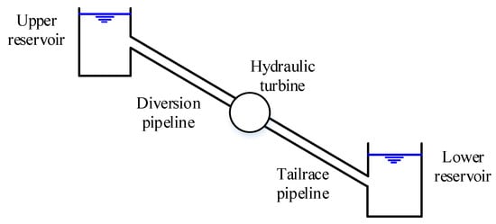
Figure 3.
Structural schematic of the power station of interest.
The system is composed of an upstream reservoir, a diversion pipeline, a hydraulic turbine, a tailrace pipeline, and a downstream reservoir. The equivalent circuit of the hydropower station system is illustrated in Figure 4. The essential parameters of the pipeline system in the hydropower station are given in Table 1.
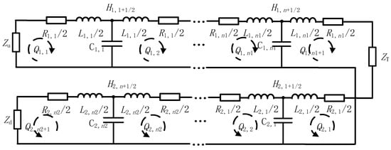
Figure 4.
Equivalent circuit of the hydraulic system of a hydropower station.

Table 1.
Parameters of the pipeline system in the hydropower station.
3.2. Frequency Response Validation of ECM
The frequency responses of the downstream end of the diversion pipe of the hydropower station in Figure 3, obtained with the proposed equivalent circuit-based impedance and the traditional continuous model [9] under different spatial steps, are displayed in Figure 5, respectively.
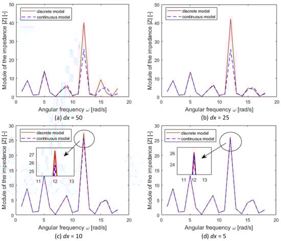
Figure 5.
Comparison of frequency responses of the pressurized pipe between the discrete equivalent circuit-based impedance method and the traditional continuous impedance method with different spatial steps.
The modeling accuracy of the discrete system models is sensitive to the choice of spatial discretization. Compared with the frequency-related analytical solutions obtained from the continuous model, the discrete impedance model tends to have more precise responses for lower frequency regions. The modeling performances for higher-order oscillations are more prone to deteriorate if dx is not small enough, as shown in Figure 5. In addition, the modeling precision for higher frequency oscillations increases when the value of the spatial step further decreases.
3.3. Free Oscillation Response Analysis of the Hydropower Station System
From Figure 5, the impedance at the upstream reservoir also can be obtained by calculating the total impedance of the series and parallel circuits using Equation (4) from the downstream side to the upstream side according to the circuit theory. Since the upstream and downstream reservoirs are considered to be two open ends, the impedances of the two reservoir boundaries are . The system stability is highly related to the oscillation characteristics of the hydraulic circuit in the power station. The oscillation patterns of different orders of the hydropower system are obtained by searching for the complex frequencies that satisfy the boundary condition via the free oscillation response analysis. The real and imaginary parts of each complex frequency represent the decay coefficient and the angular frequency of the oscillation of the corresponding order, respectively.
It is not easy to obtain the analytical solutions to the equation , for the expression of the equation is quite complex. For this reason, the well-known Newton–Raphson method [2,9,25] is used here to calculate the numerical solutions. Due to the spatial discretization of the pipeline, the mathematical expression of the overall complex frequency domain ECM model is quite complicated, and the model’s order is pretty high. Hence, it is usually rather difficult to deduce the derivative of the objective function of the optimization problem directly. For this reason, we use the first-order linear approximation of the Newton iterative method to avoid the derivation deduction process. The detailed process for this problem is shown in Figure 6.
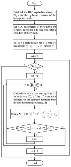
Figure 6.
Flow chart of the free oscillation responses analysis.
4. Simulation Result Analyses
Simulation experiments were conducted to reveal the features of different orders of oscillation in the hydropower station system. Since there are two pipelines in the system plant, i.e., the diversion pipeline and the tailrace pipeline, the oscillation characteristics of either pipe may be influenced by the other. In addition, the influence of the hydraulic turbine impedance on the system’s oscillation patterns needs further investigation. Note that the friction losses along the pipelines are neglected to explore the damping effect of the hydraulic turbine.
4.1. Oscillation Mode Characteristics of the Overall Hydropower Station System
It is known that the continuous model of the hydropower station system has infinite degrees of freedom. Therefore, the oscillation order for this system can be as high as infinite. However, as the proposed ECM is a discrete approximation to the system, only the characteristics of the lower orders of oscillation are precise in the modeling, as discussed in Section 2.1. Firstly, we investigate the decay coefficients of different orders of oscillation. It is found that the damping characteristics of the system oscillations when and are quite different from each other. The variation curves of the decay coefficients of the oscillations under different hydraulic turbine operating conditions with relatively small values of ZT () are illustrated in Figure 7.
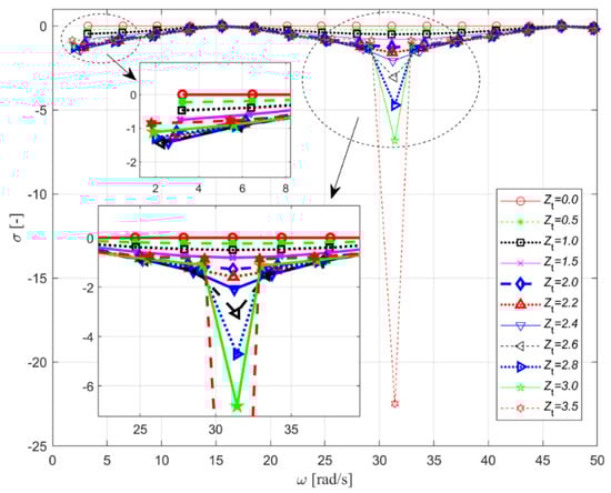
Figure 7.
Decay coefficients of different orders of oscillations under different operating conditions of the hydraulic turbine when .
Figure 7 shows that the all the decay coefficients gradually move towards zero when the angular frequency is less than 15 rad/s. At the 5th order of oscillation (about 15.58 rad/s), the decay coefficient reaches the crest and is quite close to zero (but is still negative). When the angular frequency is within 15 rad/s to 32 rad/s, the decay coefficient first decreases gradually as the angular frequency increases. At the 10th order of oscillation (about 31.16 rad/s), the decay coefficient reaches the nadir and its value is much smaller than those of the neighboring orders. Then, the decay coefficient gradually increases and reaches another crest at the 15th order of oscillation (about 46.73 rad/s), where the value at this crest is also negative and close to zero.
The decay coefficients of the oscillations of the 1st, 2nd, 3rd, 4th, 6th, 7th, 8th, 9th, 11th, 12th, 13th, 14th, and 15th orders are within the range of [−2, 0], but the value of the decay coefficient of the 10th-order oscillation varies from −22 to 0, which is quite different from the oscillations of other orders. The corresponding angular frequency ranges from 31.1 rad/s to 31.4 rad/s, which is very close to twice the base natural frequency of pipe #2 given in Table 1.
Different from that of the hydraulic turbine operating conditions with smaller values of ZT (ZT ≤ 3.5), the variation curve of the decay coefficient of the system frequency responses under the hydraulic turbine operating conditions with larger values of ZT (ZT ≥ 3.6) is illustrated in Figure 8.
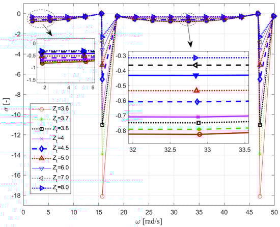
Figure 8.
Decay coefficients of different orders of oscillations under different operating conditions of the hydraulic turbine when .
Figure 8 shows that all the decay coefficients gradually increase to zero when the angular frequency is less than 15 rad/s, which is the same trend compared to that in Figure 7. At the 6th-order oscillation (about 15.70 rad/s), the decay coefficient suddenly decreases sharply to the nadir (which is much smaller than the value of neighboring orders) and then rapidly surges to a normal value (about σ = −0.28) at the 7th-order oscillation. The decay coefficient at the 6th-order oscillation ranges from −18.11 to −2.32 when ZT decreases from 8 to 3.6. While the angular frequency is within 16 rad/s to 33 rad/s, the decay coefficient at first decreases gradually as the angular frequency increases. The decay coefficient reaches the nadir at the 11th-order oscillation (about 32.88 rad/s). Then, the decay coefficient gradually increases and reaches another crest at the 15th order of oscillation (about 46.72 rad/s), where its value is negative and close to zero. Afterward, the decay coefficient suddenly decreases sharply to the unusual nadir again at the 16th-order oscillation (about 47.11 rad/s) and rapidly rises to the normal crest (within the range of [−0.26, −0.21]) at the 17th-order oscillation (about 49.85 rad/s). From Figure 8, we can also observe the angular frequencies of the two unusual oscillations (the 6th-order and the 16th-order) are 15.70 rad/s and 47.11 rad/s, respectively. Their values are close to the 1st-order (15.71 rad/s) and 3rd-order (47.12) natural frequencies of pipe #2, respectively.
It is proven that in a simple reservoir–pipe–valve hydraulic system [25], the frequencies of the free oscillation responses at the valve inlet are even harmonics when the hydraulic impedance of the valve Zv is smaller than the characteristic impedance of the pipe Zc (i.e., Zv < Zc). In contrast, the frequencies of the free oscillation responses at the valve inlet are odd harmonics when Zv > Zc. This result is quite related to our aforementioned findings. In this study, the oscillation frequency distribution obtained in the hydropower station system also presents obvious odd harmonics performance when ZT is relatively large and even harmonics performance when ZT is relatively small. The hydraulic turbine acts as the valve in the reservoir–pipe–valve system. However, the system plant is more complex and consists of multiple pipelines, the coupling effect of the pipes greatly influences the frequency responses of the overall system. The critical hydraulic turbine impedance ZT to determine the two different oscillation modes is located within the range of [3.5, 3.6]. According to the analysis above, the 10th-order oscillation when ZT ≤ 3.5 and the 6th-order and 16th-order oscillations when ZT ≥ 3.6 are considered to correspond to the natural frequencies of pipe #2.
4.2. Variation Trends of the Decay Coefficients of Oscillations of the Two Pipes
Apart from the three oscillations related to pipe #2, all other oscillations are considered related to pipe #1. The decay coefficients corresponding to different orders of oscillation related to pipe #1 under the different conditions of ZT are depicted in Figure 9. As seen in Figure 9, the decay coefficients of the 5th-order oscillation and the 14th-order oscillation are kept close to zero for all values of ZT. The angular frequencies of the two orders are 15.58 rad/s and 46.73 rad/s, respectively. These two frequencies are close to the 1st-order and 3rd-order oscillations of pipe #2. The 4th-order, 6th-order, 13th-order, and 15th-order oscillations of pipe #1 have relatively weak damping capability because the absolute values of their decay coefficients for all ZT are relatively small. The reason why they have slow convergence characteristics is that the 4th-order and the 6th-order oscillations are next to the 5th-order oscillation, and the 13th-order and 15th-order oscillations are next to the 14th-order oscillation. On the contrary, the 1st-order, 9th-order, and 10th-order oscillations have a relatively strong damping capability because the absolute values of their decay coefficients for all ZT are relatively large. The reason why they have fast convergence characteristics is that the angular frequencies of the 9th-order oscillation and the 10th-order oscillation are next to the 2nd-order oscillation of pipe #2, and the 1st-order oscillation is next to the 0th-order oscillation (i.e., the DC component).
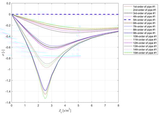
Figure 9.
Damping coefficients correspond to different orders of oscillation related to pipe #1 under the conditions of different ZT.
In addition, the decay coefficients of the oscillation modes related to pipe #1 are within the range of [−1.6, 0]. For each order of oscillation, the decay coefficient value decreases to the corresponding nadir as ZT increases when ZT is small, then the decay coefficient increases as ZT continues to increase. However, the critical hydraulic turbine impedance of the decay coefficient nadir for each oscillation order is different.
The decay coefficient variation curves of the first three orders of oscillation related to pipe #2 with different ZT are shown in Figure 10. It is seen that the 1st-order oscillation and the 3rd-order oscillation can be observed when and their decay coefficients σ nearly have the same variation trend with each other. σ increases gradually as the value of ZT increases. On the contrary, the 2nd-order oscillation is observed when , and σ gradually decreases as the value of ZT increases.
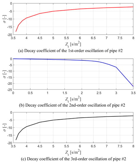
Figure 10.
Damping coefficients of the first three oscillation orders related to pipe #2 with different ZT.
4.3. Influence of the Turbine Impedance on the Oscillations Frequencies Distribution
In Section 4.1 and Section 4.2, the decay coefficients corresponding to different orders of oscillation are investigated. In this subsection, we reveal the variation trend of the oscillation frequencies of the system. From Figure 7 and Figure 8, the oscillation modes of the hydropower system are separated into two parts, i.e., the oscillations related to pipe #1 and the oscillations related to pipe #2. As discussed in Section 4.1, the oscillation frequencies’ distribution of the hydropower station system tends to present odd harmonics performance when ZT is relatively large and even harmonics performance when ZT is relatively small. The critical turbine impedance of the two oscillation patterns is within the range of [3.5, 3.6]. Therefore, the variation trends of the frequencies of different orders of oscillation of the system with different ZT are illustrated in Figure 11.

Figure 11.
Variation trends of the frequencies of different orders of oscillation of the system with different ZT.
Both frequency responses of pipe #1 and pipe #2 when ZT ≤ 2 can be considered even harmonics, although the frequencies of some oscillation orders of pipe #1 in this region are greatly affected by the coupling effect of the two pipes. On the contrary, the frequency responses of pipe #1 and pipe #2 when ZT ≥ 5 are odd harmonics for pipe #1 and pipe #2. Furthermore, an obvious frequency transition region can be observed between ZT = 2 and ZT = 5. The oscillation modes of pipe #1 gradually shift to the odd harmonics from the even harmonics as ZT increases. During this transition, the oscillation modes of pipe #1 are between the two oscillation modes. However, the oscillation modes of pipe #2 suddenly change at a critical turbine impedance (within the region of ZT ∈ [3.5, 3.6]).
5. Conclusions
An equivalent circuit-based hydraulic impedance model for a hydropower station is proposed in this paper. The free oscillation analysis of the hydraulic system of the hydropower station with this method is carried out. Several conclusions are condensed below:
(1) Compared with the analytical frequency responses of the traditional continuous hydraulic impedance method, the frequency responses of the proposed equivalent circuit-based discrete impedance method for higher frequency impulses are more prone to being inaccurate. The overall modeling accuracy is sensitive to the precision of the spatial meshing.
(2) There exists a critical hydraulic turbine impedance ZTC to determine the oscillation modes of the system. Performances of the system’s oscillation pattern for a relatively small ZT and a relatively large ZT are different. When ZT < ZTC, the oscillation modes are even harmonics, and when ZT > ZTC, the oscillation modes are odd harmonics.
(3) An obvious transition region of the frequency response for pipe #1 can be observed around the critical turbine impedance. The oscillation frequency modes of pipe #1 gradually shift to the odd harmonics from the even harmonics as ZT increases. However, the oscillation modes of pipe #2 suddenly change at a critical turbine impedance, and no transition process is observed.
Author Contributions
Conceptualization, S.Y. and Y.Z.; methodology, S.Y.; validation, S.Y., Y.Z. and J.C.; formal analysis, S.Y.; investigation, Y.S.; resources, Y.S.; data curation, S.Y.; writing—original draft preparation, S.Y. and Y.Z.; writing—review and editing, S.Y.; visualization, S.Y.; supervision, Y.Z.; project administration, Y.Z.; funding acquisition, Y.Z. All authors have read and agreed to the published version of the manuscript.
Funding
This research was funded by National Natural Science Foundation of China (grant number: 52009096), China Postdoctoral Science Foundation (grant number: 2022T150498) and the Fundamental Research Funds for the Central Universities (grant number: 2042022kf1022).
Institutional Review Board Statement
Not applicable.
Informed Consent Statement
Not applicable.
Data Availability Statement
Not applicable.
Conflicts of Interest
The authors declare no conflict of interest.
Nomenclature
| v | Flow velocity |
| a | Wave propagation speed |
| t | Time |
| x | Horizontal location along the pipeline |
| H | Piezometric head |
| Q | Discharge |
| A | Sectional area of the pipe |
| D | Diameter of the pipe |
| g | Gravitational acceleration |
| λ | Friction loss coefficient of the pipe |
| Rei | Equivalent resistance per unit length |
| Lei | Equivalent inductance per unit length |
| Cei | Equivalent capacitance per unit length |
| R | Equivalent resistance |
| L | Equivalent inductance |
| C | Equivalent capacitance |
| Zequ | Equivalent hydraulic impedance |
| s | Laplace operator, also the complex frequency |
| ZT | Turbine impedance |
| D1 | Diameter of the runner |
| n11 | Unit rotational speed |
| Q11 | Unit discharge |
| Zr | Reservoir impedance |
| hr | Piezometric head variation of the reservoir |
| Zc | Characteristic impedance of the pipe |
| ω0 | Base frequency of the pipe |
References
- Zheng, Y.; Chen, Q.; Yan, D.; Liu, W. A two-stage numerical simulation framework for pumped-storage energy system. Energy Conv. Manag. 2020, 210, 112676. [Google Scholar] [CrossRef]
- Chaudhry, M.H. Applied Hydraulic Transients; Springer: London, UK, 2014. [Google Scholar]
- Alubokin, A.A.; Gao, B.; Ning, Z.; Yan, L.L.; Jiang, J.X.; Quaye, E.K.; Evans, K. Numerical simulation of complex flow structures and pressure fluctuation at rotating stall conditions within a centrifugal pump. Energy Sci. Eng. 2022, 10, 2146–2169. [Google Scholar] [CrossRef]
- Chen, G.; Liu, C.; Fan, C.W.; Han, X.Y.; Shi, H.B.; Wang, G.H.; Ai, D.P. Research on damping control index of ultra-low-frequency oscillation in hydro-dominant power systems. Sustainability 2020, 12, 7316. [Google Scholar] [CrossRef]
- Lu, X.; Li, C.; Liu, D.; Zhu, Z.; Tan, X. Influence of water diversion system topologies and operation scenarios on the damping characteristics of hydropower units under ultra-low frequency oscillations. Energy 2022, 239, 122679. [Google Scholar] [CrossRef]
- Chen, J.; Xiao, Z.; Liu, D.; Hu, X.; Ren, G.; Zhang, H. Nonlinear modeling of hydroturbine dynamic characteristics using LSTM neural network with feedback. Energy Sci. Eng. 2021, 9, 1961–1972. [Google Scholar] [CrossRef]
- Guo, W.; Zhu, D. Critical stable sectional area of downstream surge tank of hydropower plant with sloping ceiling tailrace tunnel. Energy Sci. Eng. 2021, 9, 1090–1102. [Google Scholar] [CrossRef]
- Liu, D.; Li, C.; Malik, O.P. Operational characteristics and parameter sensitivity analysis of hydropower unit damping under ultra-low frequency oscillations. Int. J. Electr. Power Energy Syst. 2022, 136, 107689. [Google Scholar] [CrossRef]
- Yang, J.D. Applied Fluid Transients; Science Press: Beijing, China, 2018. [Google Scholar]
- Suo, L.; Wylie, E.B. Impulse response method for frequency-dependent pipeline transients. J. Fluids. Eng. ASME 1989, 111, 478–483. [Google Scholar] [CrossRef]
- Kim, S.H. Impedance matrix method for transient analysis of complicated pipe networks. J. Hydraul. Res. 2007, 45, 818–828. [Google Scholar] [CrossRef]
- Kim, S.H. Dynamic memory computation of impedance matrix method. J. Hydraul. Eng. 2011, 137, 122–128. [Google Scholar] [CrossRef]
- Kim, S.H. Address-oriented impedance matrix method for generic calibration of heterogeneous pipe matrix network systems. J. Hydraul. Eng. 2008, 134, 66–75. [Google Scholar] [CrossRef]
- Zhou, J.; Suo, L.; Hu, M. Study on self-excited vibration of hydro-mechanical system in pumped storage plants. J. Hydraul. Eng. 2007, 38, 1080–1084. [Google Scholar]
- Gong, J.Z.; Lambert, M.F.; Simpson, A.R.; Zecchin, A.C. Single-event leak detection in pipeline using first three resonant responses. J. Hydraul. Eng. 2013, 139, 645–655. [Google Scholar] [CrossRef]
- Duan, H.F.; Lee, P.J.; Ghidaoui, M.S.; Tung, Y.K. Extended blockage detection in pipelines by using the system frequency response analysis. J. Water Res. Plan. Manag. 2011, 138, 55–62. [Google Scholar] [CrossRef]
- Zhang, C.; Wang, Y.T.; Liu, Y.; Ding, W. Vulnerability Analysis of Urban Drainage Systems: Tree vs. Loop Networks. Sustainability 2017, 9, 397. [Google Scholar] [CrossRef]
- Kim, S.H.; Choi, D. Dimensionless Impedance Method for General Design of Surge Tank in Simple Pipeline Systems. Energies 2022, 15, 3603. [Google Scholar] [CrossRef]
- Paynter, H.M. Surge and water hammer problems. ASCE Trans. 1953, 146, 962–1009. [Google Scholar] [CrossRef]
- Jaeger, C. Fluid Transients in Hydro-Electric Engineering Practice; Blackie: Glasgow, UK, 1977. [Google Scholar]
- Souza, O.H.; Barbieri, N.; Santos, A.H. Study of hydraulic transients in hydropower plants through simulation of nonlinear model of penstock and hydraulic turbine model. IEEE Trans. Power Syst. 1999, 14, 1269–1272. [Google Scholar] [CrossRef]
- Nicolet, C.; Greiveldinger, B.; Hérou, J.J.; Kawkabani, B.; Allenbach, P.; Simond, J.J.; Avellan, F. High-order modeling of hydraulic power plant in islanded power network. IEEE Trans. Power Syst. 2007, 22, 1870–1880. [Google Scholar] [CrossRef]
- Zhao, Z.; Yang, J.; Yang, W.; Hu, J.; Chen, M. A coordinated optimization framework for flexible operation of pumped storage hydropower system: Nonlinear modeling, strategy optimization and decision making. Energy Convers. Manag. 2019, 194, 75–93. [Google Scholar] [CrossRef]
- Zheng, Y.; Chen, Q.; Yan, D.; Zhang, H. Equivalent circuit modeling of large hydropower plants with complex tailrace system for ultra-low frequency oscillation analysis. Appl. Math. Model. 2022, 103, 176–194. [Google Scholar] [CrossRef]
- Nicolet, C. Hydroacoustic Modelling and Numerical Simulation of Unsteady Operation of Hydroelectric Systems; Ecole Polytechnique Federale de Lausanne: Lausanne, Switzerland, 2007. [Google Scholar]
- Zhang, Y.; Zang, W.; Zheng, J.; Cappietti, L.; Zhang, J.; Zheng, Y.; Fernandez-Rodriguez, E. The influence of waves propagating with the current on the wake of a tidal stream turbine. Appl. Energy 2021, 290, 116729. [Google Scholar] [CrossRef]
- Zhang, Y.; Zhang, J.; Lin, X.; Wang, R.; Zhang, C.; Zhao, J. Experimental investigation into downstream field of a horizontal axis tidal stream turbine supported by a mono pile. Appl. Ocean. Res. 2020, 101, 102257. [Google Scholar] [CrossRef]
- Liu, D.; Li, C.; Malik, O.P. Nonlinear modeling and multi-scale damping characteristics of hydro-turbine regulation systems under complex variable hydraulic and electrical network structures. Appl. Energy 2021, 293, 116949. [Google Scholar] [CrossRef]
- Zhang, Y.; Zhang, Z.; Zheng, J.; Zhang, J.; Zheng, Y.; Zang, W.; Lin, X.; Fernandez-Rodriguez, E. Experimental investigation into effects of boundary proximity and blockage on horizontal-axis tidal turbine wake. Ocean. Eng. 2021, 225, 108829. [Google Scholar] [CrossRef]
- Wylie, E.B.; Streeter, V.L. Fluid Transients in Systems; Prentice-Hall: London, UK, 1993. [Google Scholar]
Publisher’s Note: MDPI stays neutral with regard to jurisdictional claims in published maps and institutional affiliations. |
© 2022 by the authors. Licensee MDPI, Basel, Switzerland. This article is an open access article distributed under the terms and conditions of the Creative Commons Attribution (CC BY) license (https://creativecommons.org/licenses/by/4.0/).