Article

Quantification and Removal of Volatile Sulfur Compounds (VSCs) in Atmospheric Emissions in Large (Petro) Chemical Complexes in Different Countries of America and Europe

by
Joaquín Hernández-Fernández
1,*,
Heidi Cano
2 and
Susana Rodríguez-Couto
3
1
Chemistry Program, Department of Natural and Exact Sciences, San Pablo Campus, University of Cartagena, Cartagena 130015, Bolivar, Colombia
2
Department of Civil and Environment Engineering, Universidad de la Costa, Calle 58 #55-66, Barranquilla 080002, Atlántico, Colombia
3
Department of Separation Science, LUT School of Engineering Science, LUT University, Sammonkatu 12, 50130 Mikkeli, Finland
*
Author to whom correspondence should be addressed.
Sustainability 2022, 14(18), 11402; https://doi.org/10.3390/su141811402
Submission received: 16 July 2022 / Revised: 7 September 2022 / Accepted: 8 September 2022 / Published: 11 September 2022

Abstract

:
The present research was focused on the determination and removal of sulfur-containing compounds in industrial emissions of liquefied petroleum gas purification processes in petrochemical plants located in the USA, Brazil, Colombia, Spain, and Italy. For the analysis of volatile sulfur compounds (VSCs), an improved analytical methodology was implemented. The performance of the method was evaluated for eight VSCs in a linear dynamic range between 0.1 and 50 ppm. The concentrations of the eight VSCs in the deethanizer affluents ranged from 11 to 49 ppm for all the studied plants, which exceed the limits specified by institutions and administrations in occupational health and safety. The concentrations of the eight VSCs in the splitter affluents were lower than 4 ppm for all the considered plants. The emissions from each column depended upon its operating rate, with the highest concentrations estimated at 45 TM kg−1 and the lowest ones at 25 TM kg−1. A zeolite-packed prototype column was fitted at the outlet of the splitter and deethanizer columns to reduce the environmental effect of the examined VSCs. This technique was verified and put into practice on an industrial scale, obtaining VSC removal percentages of between 85 and 91%.

1. Introduction

Volatile sulfur compounds (VSCs) are colorless compounds with different levels of toxicity and odor thresholds depending on their chemical composition. Dimethyl sulfide ((CH3)2S), carbon disulfide (CS2), hydrogen sulfide (H2S), ethylmercaptan (CH3CH2SH), methylmercaptan (CH3SH), propylmercaptan ((CH3(CH2)2SH), carbonyl sulfide (COS), and butylmercaptan ((CH3(CH2)3SH) belong to the above-mentioned family of compounds. They represent pollutants produced in many industrial facilities such as paper mills and wastewater treatment plants (WWTPs). They are also found in refineries, plants devoted to food and natural gas processing, as well as in the purification of liquefied petroleum gas (LPG), petroleum, and crude [1]. Some of these compounds are used in the intermediate stages of insecticides, syngas, plastics, and antioxidant manufacturing and as a natural odorizer warning [2,3].
There is no information on the emission levels of VSCs in the LPG purification stages on an industrial scale. This absence stimulated the effort to develop analytical methodologies, as well as sampling plans and procedures to measure their environmental impact of LPG-related operations that are primarily focused on refineries and a wide range of petrochemical businesses, which use petroleum as a raw material. Petrochemical and petroleum refineries generate a variety of pollutants into the atmosphere (nitrogen oxides (NOx), lead (Pb), sulfur oxides (SOx), carbon monoxide (CO), air particulate matters (PM), ozone (O3), and volatile organic compounds (VOCs)) that can have a significant impact on human health, particularly for those who live nearby [4,5,6,7].
Some of these reduced sulfur compounds are frequently detected in the environment (e.g., H2S, CH3SH, (CH3)2S and dimethyl disulphide (DMDS)) [8], generating a strong noxious odors, even at concentration levels below ppb [9], and the exposure to low concentrations of VSCs causes headache, fatigue, and irritation of the eyes, nose, and throat, and can even cause death from respiratory paralysis [10]. As a result, it is vital to monitor and manage the processes that make these compounds. Air pollution is a serious environmental public health issue, according to epidemiological research, which has been proven by several studies that have indicated that exposure to VSCs in the air is related to various adverse effects such as asthma, lung cancer, chronic obstructive pulmonary, and cardiovascular disease [11,12].
Different investigations were carried out in areas surrounding petrochemical sectors to evaluate the impact of their emissions on the health of the nearby population. Thus, Xu et al. [13] found that pregnant women who live near a big petrochemical complex that generated H2S emissions in Beijing have a higher chance of miscarriage. Camargo et al. [14] compared the frequency of chronic autoimmune thyroiditis between those who lived near the Capuava petrochemical complex and those who lived in a control region (São Bernardo do Campo), both urban districts in the São Paulo metropolitan area, Brazil, and found a higher prevalence of thyroiditis in those people. White et al. [15] found that asthma symptoms of children living near a petrochemical plant (Cape Town-South Africa) were associated to exposure to refinery pollutants. Moraes et al. [16] carried out cross-sectional research on children’s wheezing (0–14 years old) who lived near the Guamaré-Brazil petrochemical plant and found that respiratory symptoms were related to living in the plant vicinity. In Italy, Rusconi et al. [17] evaluated the oxidative stress, lung function, and inflammation and in children aged from 6 to 14 years old living in an area contaminated by petrochemicals in Sarroch, Italy. They reported that the older children, who had lived more time near that polluted zone, presented reduced lung function and increased inflammation. Rovira et al. [18] identified respiratory symptoms and asthma in children aged from 6 to 7 years old and in adolescents aged from 13 to 14 years old who lived near the Tarragona petrochemical complex in southern Europe. Additionally, in Sarroch, Italy, Barbone et al. [19] found that children of 8–14 years old who lived near a refinery had short-term effects of reduced lung function and increased inflammation of the respiratory tract by exposure to VSCs (e.g., SO2). In Korea, the prevalence of hypertension in 69.2%, coronary artery disease in 13.9%, cerebrovascular disease in 24.8%, diabetes in 24.5%, arrhythmia in 1.3%, psychoneurotic disorder in 65.7%, and nervous system and sensory organ disorders in 72.4% of the workers exposed to concentrations higher than 10 ppm of CS2 was observed [20].
The maximum exposure concentration allowed by United States Occupational Health and Safety Administration (OSHA) is of 20 ppm for H2S and CS2. An exposure of 10 ppm [21] was recommended by the United States’ National Institute for Occupational Safety and Health (NIOSH). The threshold limit value recommended by the American Conference of Governmental Industrial Hygienists (ACGIH) is 1.0 ppm/8-h and 5.0 ppm for a short-term exposure limit. In the case of CH3 (CH2)3SH, CH3(CH2)2SH, CH3CH2SH, and CH3SH, their allowed maximum concentrations in the environment are less than 10.0 ppm in their liquid phase and should not exceed 1.1 ppm in their gas phase according to NIOSH [22,23].
The removal of VSCs is of significant practical importance for both industrial production and environmental protection, which has driven research interest in the development of new measurement methodologies and sustainable disposal systems on an industrial scale. The techniques traditionally used by industry for desulfurization include adsorption [24,25], cryogenic processes [26], absorption [21,27], and more recent techniques combine biological oxidation and electrochemical purification processes [23,28]. However, all the above-mentioned techniques suffer from several drawbacks such as large capital outlays and severe secondary environmental pollution generated by other chemicals present in the environment when they react with the compounds released from industrial processes and cumbersome equipment. Desulfurization is a common part of LPG purification, and it may reduce H2S levels to below 10 ppm [29]. However, this process has no effect upon the removal of organic sulfur like CH3SH and COS [30]. The organic sulfur molecule CH3SH is the most difficult to remove from gas. Adsorbents such as iron oxides, zinc, zeolites and activated carbon are frequently employed to remove CH3SH [31,32].
We used a systematic sampling method to obtain gas samples from five industrial LPG purification procedures for this investigation of 5 different polypropylene production petrochemical plants with similar operating technologies located in Spain, the USA, Brazil, Italy, and Colombia. The samplings were carried out in the deethanizer and splitter columns where the pollutants are released into the environment, and the concentrations of VSCs, corresponding to H2S, COS, CS2, (CH3)2S, CH3(CH2)3SH, CH3(CH2)2SH, CH3CH2SH, and CH3SH, were measured. Further, a prototype quartz tube column packed with synthetic zeolite was built to improve the removal of VSCs. The emission profiles of the VSCs were evaluated in the facilities to know their formation mechanism. The emission factors and emission amounts of H2S, COS, CS2, (CH3)2S, CH3(CH2)3SH, CH3(CH2)2SH, CH3CH2SH, and CH3SH under a toxic equivalence scheme (TEQ) were estimated to provide a first data on VSC emissions from LPG purification plants in Spain, the USA, Brazil, Italy, and Colombia.

2. Materials and Methods

2.1. Calibration

In the present investigation we have worked with 8 primary standards and 40 secondary standards. A standard for mixing of VSCs was certified by Airgas USA LLC (Sacramento, CA, USA), with concentrations of 50 ppm CH3(CH2)3SH (STDA 1), 50 ppm CS2 (STDA 2), 50 ppm COS (STDA 3), 50 ppm (CH3)2S (STDA 4), 50 ppm CH3CH2SH (STDA 5), 50 ppm H2S (STDA 6), 50 ppm CH3SH (STDA 7), and 50 ppm CH3(CH2)2SH (STDA 8), in propylene gas balance.

2.2. Calibration Curve

The multi-point calibration curve was created using a VSCs mix standard. The desired concentration ranges in propylene gas balance are presented in Table 1.

2.3. Sampling Points and Sample Collection

The samplings were carried out in 5 petrochemical polypropylene producing plants located in Spain, the USA, Brazil, Italy, and Colombia. Each of these plants has independent processes for the purification of LPG, represented in Figure 1, which will be used later as raw material in the synthesis of polypropylene. The present investigation focused on the stages 2 and 3 which corresponded to the deethanizing column, which separates the most volatile components from LPG, and the splitter column, which separates propylene from propane respectively. In Figure 1 the sampling points are identified with the image of the metal cylinder. These sampling points (deethanizer column affluents valve, splitter column affluent valve, zeolite–deethanizer column valve, and zeolite–splitter column valve) are not monitored with high frequency in the process controls, and water and metallic particles are observed. To eliminate the particles in the samples of interest, a filter from the NUPRO–Swagelok family was installed [33]. The NUPRO “F” from 7 to 15 microns were used in the gaseous samples and the NUPRO “FW” from 2 to 7 microns were used for the liquefied samples [34]. The gas samples were obtained isokinetically with an Isostack G4 1.4 mc automated sampler, according to Method 23 (US EPA, 2017) (Tecora, Cogliate, Italy). A quartz filter and a 1000-mL stainless steel cylinder, both deactivated and with an interior coating of sulfinert to inhibit VSCs adsorption and absorption, were used to collect both particle and gas phases for each gas sample. The cylinder was configured with a relief valve for pressures between 300 and 400 psi [34]. The sample volumes were adjusted to meet standard conditions of 25 °C, 760 mmHg, dry gas basis, and operational oxygen concentration. The isokinetic for the gas sample in this investigation varied from 94 to 103 percent, which is within the US EPA Method 23 permissible limit. Gas samples were obtained from the splitter columns and the top of the deethanizer. The investigation was carried out when the deethanizer and splitter columns operated at 25, 35, and 45 TM kg−1. The samples from the deethanizer column, the zeolite column coupled to the deethanizer, the splitter column, and the zeolite column coupled to the splitter column for the plants in Spain, the USA, Brazil, Italy, and Colombia were identified as DS, ZDS, SS, ZSS, DU, ZDU, SU, ZSU, DB, ZDB, SB, ZSB, DI, ZDI, SI, ZSI, DC, ZDC, SC, and ZSC, respectively. Each identification was numbered 25, 35, and 45 depending on its operating rate at the time of sampling. The basic information on the operational conditions of the columns in the investigated plants and the identification of each sampling point are shown in the Supplementary Information (Table S1). Each monitoring was carried out in triplicate and the study involved a total of 180 samples. The cylinders were promptly transported to each plant’s quality assurance laboratory for LPG analysis. The gas sample was done under the industrial plants’ typical working circumstances. The sample time was usually between 3 and 4 h.

2.4. Chemical Analysis

The chemical analysis of the samples was carried out by chromatography following the method developed by [35]. The analyses were performed using an Agilent 7890B C (Santa Clara, CA, USA), which worked with 1 detector, 4 valves, 5 columns, and front and back split/splitless injection ports. The inlet front operating conditions were: 7.88 psi, 250 °C, and 33 mL min−1. The inlet back operating conditions were 11.73 psi, 250 °C, and 13 mL min−1 [35]. The GC worked with He as flow of 2.8 mL min−1. The total chromatographic run to identify the VSCs was 37.14 min. A dynamic blender, Wasson-ECE instrument (series # 150911DB) (Fort Collins, CO, USA), with a gas sample intake (1/16” A-lok bulkhead), a gas sample vent, a diluent gas controller, a 2u union filter (part number 1526), and blank capillary tubing of 50 cm × 0.05 mm (part number S0168), was used to dilute LPG standards [34]. The oven temperature starts at 40 °C × 3 min, increasing to 60 °C at 10 °C min−1 × 4 min and finally, increasing to 170 degrees at a rate of 35 °C min−1 for 25 min.
In the Supplementary Information (Figure S1), the chromatographic system’s configuration is presented. The valves 6, 7, 8, and 9 were involved in the VSC trace analysis. Valves 7 and 8 had 0.25 mL loop capacity. The columns are specified in Table 2 and follow the process described by [34]. Total ion current (Scan) and the select ion monitoring (SIM) were used to record the chromatogram [36].
In the Supplementary Information (Figure S1), it can be observed that at the “off” position, the dynamic blender samples were routed via the R column and the vaporizer to purge the loops of valves (6, 7, 8, and 9). In columns 1 to 5, and the particle trap, compounds that may cause interference in the VSC detection and quantification system were retained. The analysis began by turning valve 6 to the ON position, allowing the sample to access the system. Then, in order for the sample to flow to column 1, valve 7 was switched to the ON position. This kept the LPG and other chemicals with similar or higher boiling temperatures from affecting the MS’s tungsten filaments’ sensitivity or life duration. The valve 8 was switched on a few seconds later, allowing the material to be delivered to column 3 [34]. After a few minutes, the valve 9 was opened, enabling the mixture to proceed to column 5, where the VSCs were separated. The detector’s solitary turn-on time was 32 min. The chromatogram for MS is shown in Figure 2.

2.5. Validation Method

The linearity of the working ppm of the VSCs was determined. Because the quality of the data was dependent on the dynamic blender’s operation and functionality, its operation was confirmed based on its linearity. Six concentration levels were used for each of the VSCs of interest to assess linearity. Linearity was tested visually as analyte ppm vs response, and it was expressed using the R2 [34].
Precision was measured as a relative standard deviation in terms of repeatability and intermediate precision. Repeatability for 0.1, 2.24, 5, 10, 20, and 50 ppm CH3(CH2)3SH; 0.1, 1.93, 5, 10, 20, and 50 ppm CS2; 0.1, 1.48, 5, 10, 20, and 50 ppm COS; 0.1, 1.56, 5, 10, 20, and 50 ppm (CH3)2S; 0.1, 1.56, 5, 10, 20, and 50 ppm CH3CH2SH; 0.1, 0.85, 5, 10, 20, and 50 ppm, H2S; 0.1, 1.22, 5, 10, 20, and 50 ppm CH3SH; and 0.1, 1.88, 5, 10, 20, and 50 ppm CH3(CH2)2SH was accomplished by injecting three degrees of concentration into the LPG matrix six times. Each injection was carried out on the same day, by the same operator, using the same apparatus. The results of six injections for all standards during ordinary operation of the system over ten days were used to compute intermediate precision. The relative error was used to indicate measurement precision. If the total average calibration levels were less than 20%, analyte intra- and inter-day accuracy was declared verified [37]. The accuracy and veracity of most validation techniques described in the literature were calculated by making at least six measurements per concentration. As a criterion of approval, a deviation of less than 15% from the predicted value is indicated [37]. The calculations were made using relative errors (Er). Accuracy was considered good if the bias was <15% and acceptable if it was between 15–20%.

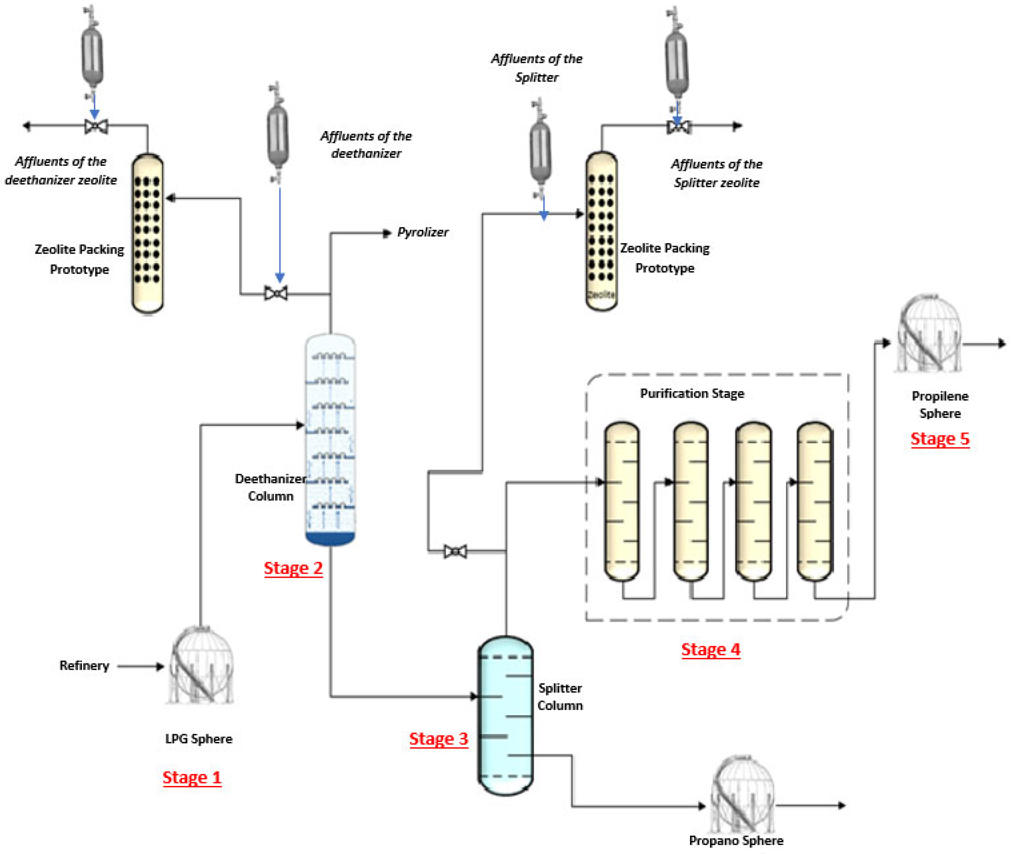
2.6. Prototype Zeolite Column and Removal of VSCs

A zeolite R3-12 (BASF) with a composition of 40% CuO, 40% ZnO, and 20% Al2O3 was used. This zeolite was in the form of 5 × 3 mm tablets and had an apparent density of 1250 kg m−3. Its thermal stability was higher than 350 °C. Therefore, in order to avoid degradation of the zeolite, operating conditions lower than 250 °C were defined. For the removal the VSCs, 150 mg of R3-12 was placed in the center of a quartz-tube and held in place by quartz wool plugs at both ends. The length of the tube was 89 mm, its outer and inner diameter were of 6 and 4 mm [33]. Prior to use, the zeolites were purged with He a 20 mL min−1 for 25 min and 35 °C. The gases released did not contain VSC residues, leading to the conclusion that these contaminants were absent in the zeolites. The removal efficiency of the VSCs for the prototype zeolite columns coupled to the deethanizer column and the splitter column in the plants of Spain, the USA, Brazil, Italy, and Colombia was independently evaluated to guarantee the correct performance of the zeolites. Blanks were prepared for all 6 concentration levels of each VSC, and the RSD was evaluated in triplicate. Successive blank analyzes let you know if there are desorption or chemical releases over time, as the bed or column can shed impurities over time, and this procedure lets you know how stable the bed is.

3. Results

3.1. Precision, Accuracy, and Linearity of the Chromatographic Method: Intra-Day and Inter-Day/Inter-Country Measures

The intra-day and inter-day inter-country accuracy of the chromatographic technique was investigated. To conduct the intra-day precision investigation, 6 duplicates of each VSC of interest were analyzed on the same day. Inter-day inter-country precision was evaluated employing distinct people, on different days in Spain, the USA, Brazil, Italy, and Colombia. The ppm values were determined according to Table 3. The results showed the precision of the method used for all the concentration ranges. For all the VSCs the intra-day precision was lower than 2.42%, and the inter-day inter-country precision was lower than 2.77%. External influences had no substantial impact on the procedure, according to the results. The intra-day and inter-day inter-country accuracy, for all concentration ranges and for all VSCs, was lower than 1.66%. This indicated that the measurements in Spain, the USA, Brazil, Italy, and Colombia were dependable and not affected by external factors or other non-instrumental differences.
The calibration curves of the 8 concentration levels for each VSC showed linearity between 0.1 and 50 ppm. The correlation coefficients (R2) in the plants of Spain, the United States, Brazil, Italy, and Colombia were all greater than 0.9999, suggesting remarkable linearity and independence of the matrix component. Detailed results for each analyte concentration are included in the Supplementary Information (Figure S2).

3.2. Performance Evaluation of Zeolite Filled Column Prototype Using Multiple VSC Standards

Efficiency was evaluated for each of the VSCs, and the concentrations indicated in Table 4 ranged between 80 and 89% for concentration ranges from 0.1 to 50 ppm. In a previous study, it was reported that the performance of the zeolite used in the present study showed a maximum percentage removal of arsine and phosphine of 99.9% [33]. The removal efficiencies achieved for the studied VSCs were also much higher than the 24 and 40% values obtained by terbuthylmercaptane in other investigations when using the hybrid polymers NaY/CA and UiO-66 (Zr)/CA as adsorbents, respectively [12].

3.3. Quantification and Removal of VSCs

The mass concentrations of VSCs in the tested gas samples from the LPG purification industries are summarized in Table 5.

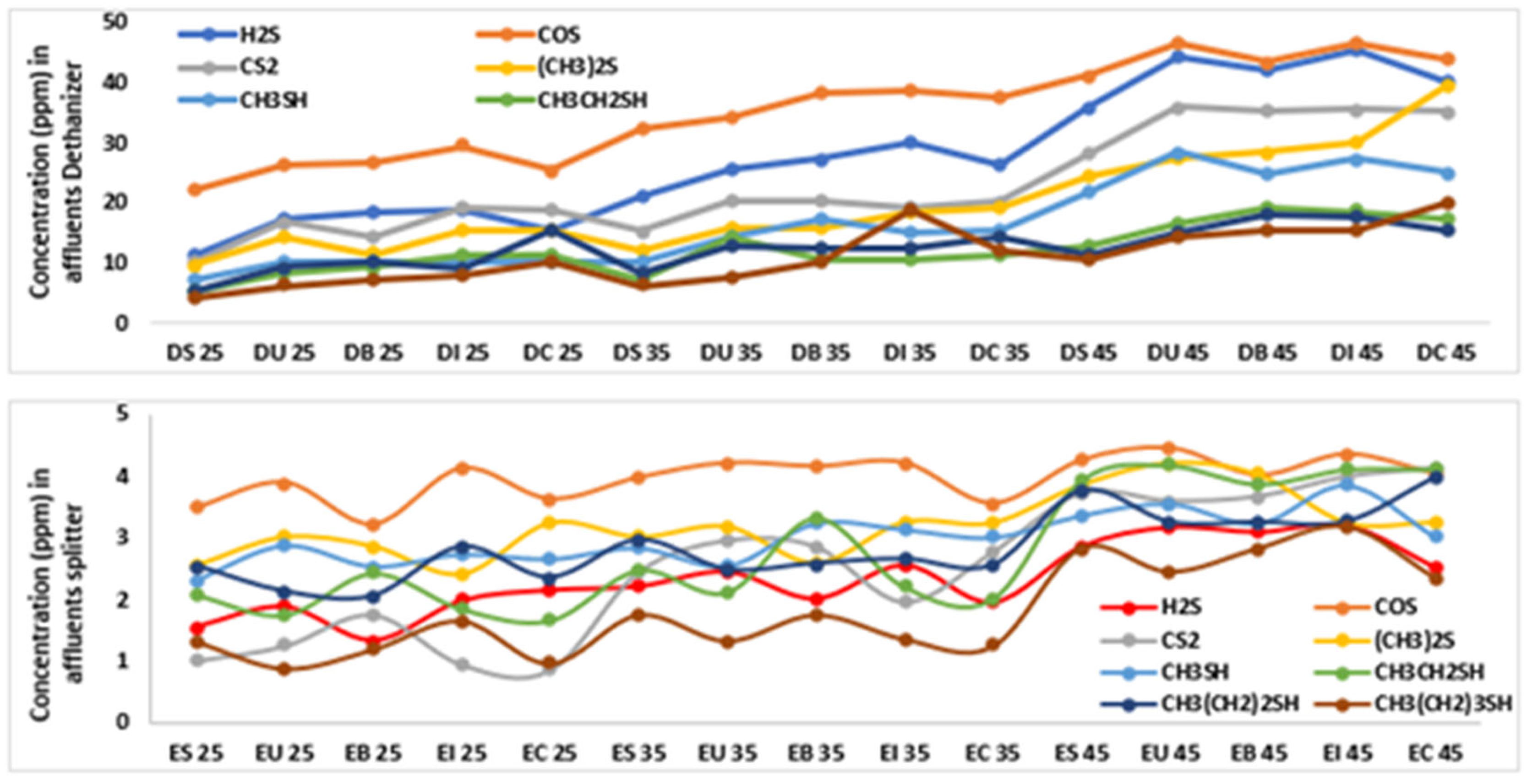
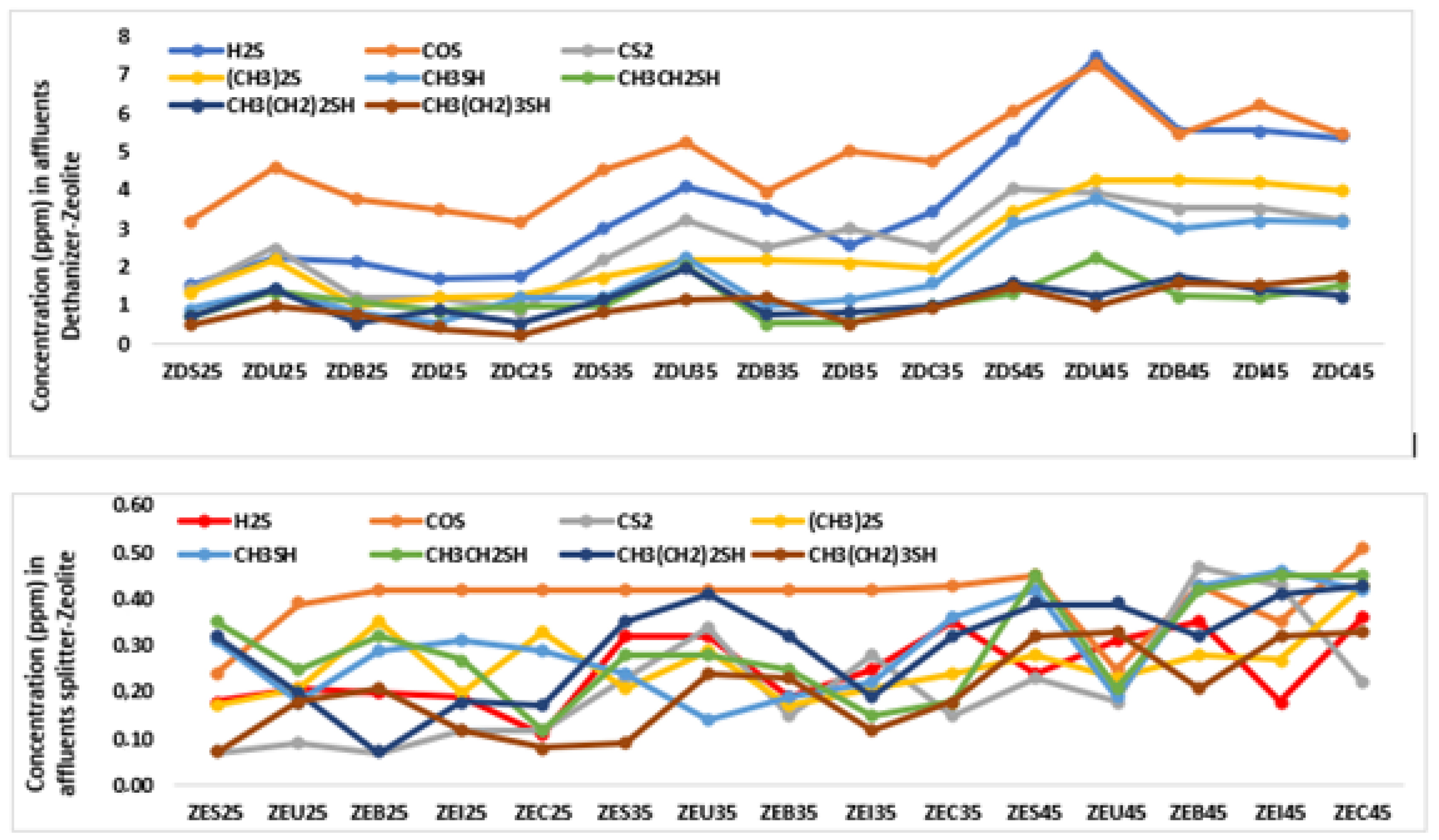
3.3.1. Deethanizer Column

In general, as shown in Table 5, the VSC concentrations in the gases of the LPG purification process were in the order deethanizer column > splitter column > zeolite column attached to the deethanizer > zeolite column attached to the splitter. The highest levels of VSCs were found in the emissions generated in the deethanizing columns in all the studied plants. The deethanizing columns worked at 25, 35, and 45 kg h−1 rates. Under these conditions, the highest VSC emissions were obtained at 45 kg h−1. Thus, at this 45 kg h−1 rate, the deethanizer columns in the plants in the United States and Italy showed the highest VSC values, with a concentration of 46.52 ppm for the DU 45 and DI 45 samples. Hence, they exceeded the maximum exposure limits (10 and 20 ppm) allowed by NIOSH, OHSA, and ACGIH [10,21,22]. The results of VSCs obtained in the deethanizer shows the importance of implementing a removal system that minimizes the impact of VSCs towards the environment and the health of workers and surrounding communities. The lowest concentrations of VSCs were found at operating rates of 25 kg h−1 in the production plant in Spain (DS 25; 4.25 ppm), followed by the US plant (DU 25; 6.25 ppm), then the Brazil plant (DB 25; 7.35 ppm), followed by the Italy plant (DI 25; 7.89 ppm) and finally by the Colombia plant (DC 25; 10.24 ppm). VSC concentrations showed significant reductions after coupling the zeolite column prototype to the top of the deethanizer column. These reductions were observed in all the rates operating the spine (i.e., at 25, 35, and 45 kg h−1) and in each of the countries where this research was carried out. The lowest values of VSCs were observed when the column worked at a rate of 25 kg h−1 in the plants of Colombia, Italy, and Spain, with values of 0.24 (ZDC 25), 0.42 (ZDI 25), and 0.51 ppm (ZDS 25), respectively.
The efficiency in the plants in Italy and Colombia showed the highest removal efficiencies of VSCs with average values of 92% at an operating rate of 25 kg h−1. These values were related to the high selectivity of the zeolites and the absence of impurities or inhibitors of a polar chemical nature in the raw material (GLP) of each country. The increase in the operating rate up to 35 kg h−1 showed the best efficiencies for VSC removal in the plants of Brazil, Italy, and Colombia, with removal values of approximately 90%. At 45 kg h−1 the highest VSC removal efficiencies were 88% in the plants in Brazil, Italy, and Colombia. Statistical evaluation of the removal efficiency of VSC in plants in Spain, the USA, Brazil, Italy, and Colombia showed RSD values of 0.24, 4.41, 0.72, 1.56, and 2.39, respectively, indicating that the spinal operating rate did not exert a strong effect on the removal of the VCSs. This reflects the great variability in the emissions of these pollutants and shows that their level of environmental impact is dependent upon the operating rate of these columns.

3.3.2. Splitter Column

As can be seen in Figure 1, the splitter columns received the flow of LPG from the deethanizing column. Therefore, operationally, it was expected that this flow of LPG had a lower VSC content. As shown in Table 5, all concentrations detected in Spain, the USA, Brazil, Italy, and Colombia, at the operating rates of 25, 35, and 45 kg h−1, were lower than the maximum permit limits and below the minimum values established by OSHA, NIOSH, and ACGIH [10,21,22]. Thus, the highest values were 4.45 ppm (EU 45), and the lowest concentrations were 0.86 ppm (EC 25).
The efficiency of columns with zeolite in all plants showed high removal efficiencies of VSCs with average values of 90% at all operating rates. For these emissions from the prototype column coupled to the splitter column lowest values of VSCs were observed when the column worked at a rate of 25 kFg h−1 in the plants of Spain, the USA, Brazil, and Colombia with values of 0.07 ppm (ZES 25, ZEU 25, ZEB 25, and ZEC 25). These effluents presented a much lower risk to the environment and the health of the personnel, demonstrating a significant commitment to the preservation and conservation of the environment and health.

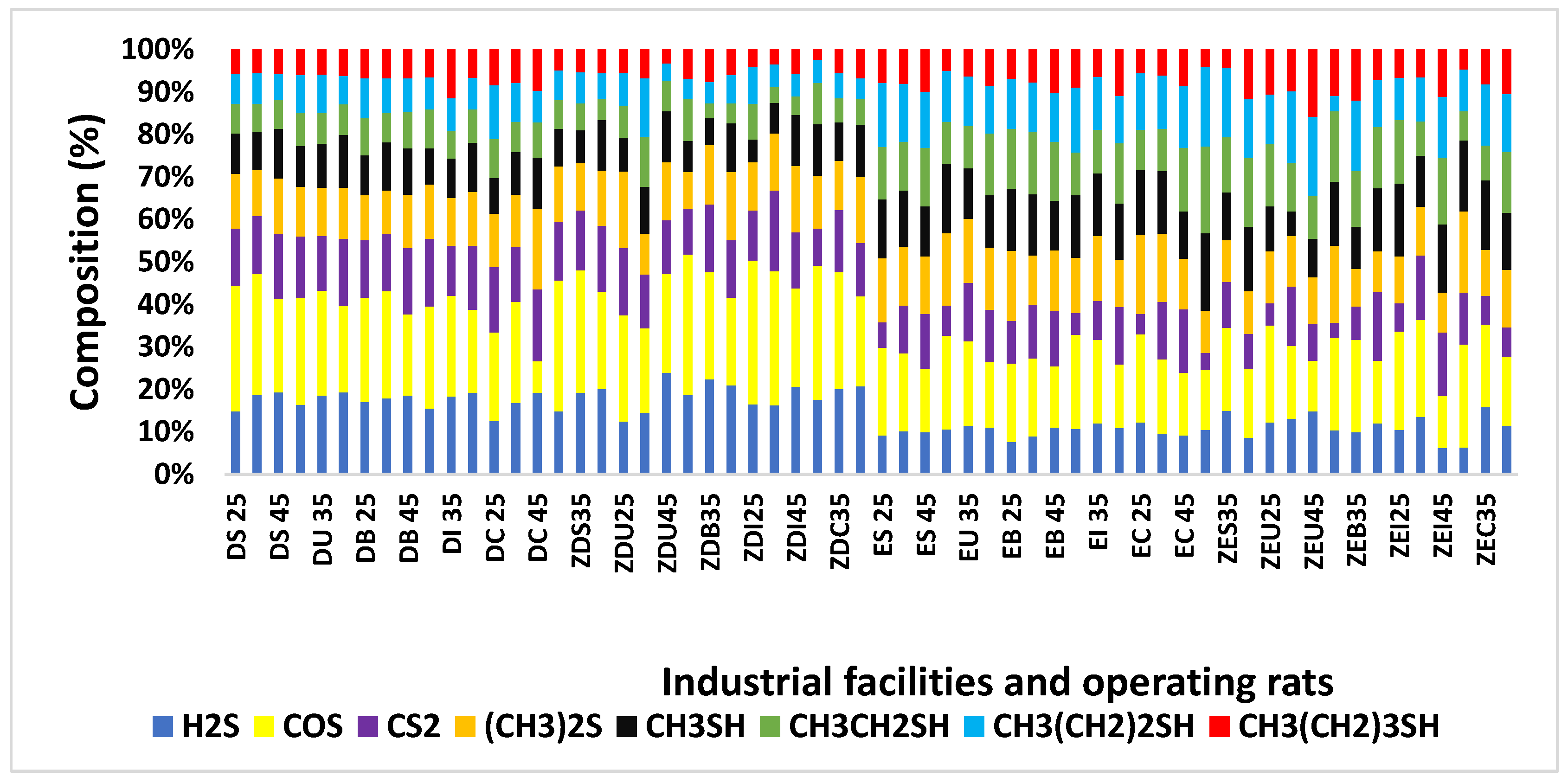
3.4. Industrial Emission Profiles of VSC

As far as we know, VSC profiles in emissions from different LPG purification processes of multiple industrial sectors in Spain, the USA, Brazil, Italy, and Colombia were not reported before this study. H2S, COS, and CS2 were the most important contributors to VSC concentrations in most samples and their concentration levels depended on the operating rate of each column. For the deethanizing columns of Spain, the USA, Brazil, Italy, and Colombia, the VSC profile maintained the following order COS ˃ H2S ˃ CS2 ˃ (CH3)2S ˃ CH3SH ˃ CH3CH2SH ˃ CH3(CH2)2SH ˃ CH3(CH2)3SH. The contributions of the 8 VSCs and the concentrations in the gas samples are presented in Figure 3. The most important contributors of H2S in the samples of interest ranged between 19 and 24%. A contribution of 19.3 ± 4.2% was identified in the samples from Spain, the USA, and Italy when the column worked at an operating rate of 45 kg h−1 (DS 45, DU 45, D I45, and ZDS 35), contributions of 21.4 ± 8.2% in samples ZDS 45, ZDB 45, ZDI 45, ZDC 35, and ZDC 45 corresponding to the plants in Spain, Brazil, Italy, and Colombia. A contribution of 22 ± 6.1% was found in the Brazilian sample ZDB 35. The highest contribution was 24 ± 7.5% in the ZDU 45 sample at the USA plant. In the deethanizer columns and at the three operating rates, the concentrations of H2S in the plants of the 5 countries varied between 11.25 and 45.51 ppm, as shown in Figure 4. These concentrations exceeded the maximum exposure limits of 10 and 20 ppm allowed by NIOSH, OHSA, and ACGIH [10,21,22,38]. These results also exceeded the baseline values of H2S in the air which ranged between 0.00011–0.00033 ppm, and in urban areas it was as high as 0.001 ppm [39]. These emissions from the deethanizer also exceeded the values of 0.09 ppm identified in places near cities [40]. They also exceeded the maximum reported measurements of 7.31 × 10³ ppm in animal feeding operations, 1.11 × 10³ ppm in wastewater, 2.64 × 10³ ppm for decomposition, 7.98 × 10 ppm in geothermal, 4.37 × 10² ppm in energy production, and 3.80 × 10³ ppm for plant emissions and sulfur-bituminous concrete emissions [39,41,42]. In order to minimize the impact to the environment and health that such VSC concentrations could cause, a column of zeolites was coupled to each deethanizer and splitter column.
The H2S values in samples from the splitter column were lower than 3.2 ppm, at all sampling points. The highest values prevailed when the column operated at 45 kg h−1 (EU45: 3.2 ppm; EI45: 3.2 ppm), and the lowest concentrations were found at 25 kg h−1 (ES25: 1.5 ppm; EB25:1.3 ppm) rate, see Figure 4. These ranges of 1.3–3.2 ppm were lower than those established by OSHA, NIOSH, ACGIH, but even so, the zeolite column was coupled to guarantee cleaner emissions and less impact on the health and the environment.
The COS at all the sampling points indicated three trends in its contribution to the samples, a contribution between 10 and 20%, the next between 20 and 30%, and the last one higher than 30%. The contributions higher than 30% were identified in the samples from Spain (DS25), Brazil (DB25), Italy (DI25, ZDI35), and Colombia (DC25). In the deethanizers and at the operating rates of 25, 35, and 45 kg h−1, the COS concentrations in the 5 petrochemical plants varied between 22.31 and 46.52 ppm. These concentrations exceeded the values of 10 and 20 ppm as well as the maximum exposure limits allowed by NIOSH, OHSA, and ACGIH [10,21,22,38]. During our research, we discovered that seven surface sites in the northern hemisphere, spread across America and Europe, had the greatest COS concentration in comparison to the average value of 0.00048 ppm [43]. They were also higher than that found in Brazil (All Saints Bay region) where COS concentrations during 1996 were approximately 0.008 ppm when originating from a petrochemical complex. The values of our research exceeded those obtained for southern Europe (0.00022 ppm) in samples taken between 1996 and 1998 [44]. The concentration of the studied sampling points also exceeded the annual mean COS in Ahmedabad (India) of 0.00083 ppm, which was much higher than the free troposphere measurements for the northern hemisphere at the time [45]. The behavior of COS in the splitter column presented a trend similar to that obtained in the affluents of the deethanizer column after being treated in the zeolite column. All H2S values obtained were less than 5.0 ppm. The lowest emissions were quantified in Spain and Brazil (ES25: 3.48 and EB 5: 3.21 ppm) and the highest emissions in Italy and the USA (EI45: 4.35 and EU45: 4.45 ppm) at operating rates of 45 kg h−1. These value ranges of 3.2–4.4 ppm of COS were higher than those established by OSHA, NIOSH, ACGIH, but higher than 0.00022 ppm, 0.00048 ppm, and 0.00083 ppm in Brazil (All Saints Bay region), Ahmedabad (India), and southern Europe [43,44,45]. These low concentration levels reported in the literature led to the implementation and coupling of the zeolite column in the splitter column to guarantee cleaner emissions.
CS2 and (CH3)2S were identified at all sampling points and the highest concentrations were detected in the USA and Colombia plants with values of 35.94 (DU 45) and 39.56 ppm (DC 45), respectively (see Figure 4). With values of such as those identified for CS2, the generation of daily explosions in viscose production industries has been reported in the literature [46,47]. In Europe (5 ppm) and the United States (20 ppm), these CS2 exposure levels were significantly beyond the allowed threshold limit (TWA). Experts now advocate even lower limit limits, ranging between 1 and 10 ppm, based on multiple epidemiological research [48,49]. These CS2 compounds can generate toxic effects such as neurofilament axonopathies [50], affecting both sensory and motor neurons [51,52,53] as well as vascular complications [54,55,56]. Emissions generated by petrochemical plants and rayon manufacturing in Korea showed that in workers occupationally exposed to levels of CS2 ≥ 10 ppm, the prevalence of diabetes was 24.5% among 633 workers, indicating that a long-term exposure to CS2 could result in an increased risk of diabetes [20]. The contributions of CS2 and (CH3)2S to each sample depended on the sampling point and the country where the sample was taken. In Figure 3, it is observed that the maximum and minimum contribution of CS2 in the deethanizing columns were identified in the samples from the plant in Italy (DI25: 16 ± 2.8% and DI35: 12 ± 2.3%). For the (CH3)2S, the highest contribution was in the Colombia plant (DC45: 17 ± 5.1%) and the lowest contribution in the samples from the Brazil plant (DB35: 10 ± 3.4%). The maximum and minimum CS2 emissions were quantified in Colombia (EC25: 0.86 ppm and EC45: 4.12 ppm, respectively). For (CH3)2S, the lowest emissions were observed in Italy (EI25: 2.41 ppm) and the highest ones were observed in the USA (EU 45: 4.21 ppm). The concentration generated by the splitter columns was lower than the recommended value of 10 ppm [48,49] and those established by OSHA, NIOSH, and ACGIH, but higher than 0.00022 ppm, 0.00048 ppm, and 0.00083 ppm [43,44,45].
The mercaptan family CH3SH, CH3CH2SH, CH3(CH2)2SH, and CH3(CH2)3SH was quantified at all sampling points of the deethanizer. The species with the highest concentration was CH3SH with 28.42 ppm in a sample from the plant in the USA (DU45), while the one with the lowest concentration was CH3(CH2)3SH in the plant in Spain (DS45: 4.25 ppm). The concentration range of CH3SH, CH3CH2SH, CH3(CH2)2SH, and CH3(CH2)3SH in Spain were 7.15–21.87, 5.32–12.78, 5.34–11.19, and 4.25–10.73 ppm, respectively (Figure 4). It was observed that CH3SH was the compound present in the highest concentration and CH3(CH2)3SH was the most diluted one. In the USA, the ranges of CH3SH, CH3CH2SH, CH3(CH2)2SH, and CH3(CH2)3SH were 10.12–28.42, 8.25–16.45, 9.41–15.24, and 6.25–14.25 ppm, respectively. The highest concentration observed was 28.42 ppm for CH3SH and the lowest one was 6.25 ppm for CH3(CH2)3SH. In Brazil, the ranges determined were 10.14–24–95, 9.45–19.24, 10.12–18.19, and 7.35–15.35 ppm, respectively. As in the previous plants, CH3SH and CH3(CH2)3SH were the ones with the highest and lowest concentration. In Italy, the ranges were 10.35–24.35, 11.32–18.65, 9.21–17.73, and 7.89–18.71 ppm for CH3SH, CH3CH2SH, CH3(CH2)2SH, and CH3(CH2)3SH, respectively. In this plant, CH3SH and CH3(CH2)3SH also presented the highest and lowest concentration, with values of 24.35 and 7.89 ppm. In Colombia, the values of these mercaptans were as follows: 10.24–25.16, 11.25–17.35, 15.45–15.36, 10.25–20.12 ppm. CH3SH presented the highest concentration in Colombia (DC45: 25.16 ppm) and the lowest concentration in the USA (DU25: 10.12 ppm). These mercaptan families are characterized by their odor thresholds. As a result, the olfactory threshold for CH3SH is extremely low, and it may be detected at only 0.00002 ppm in air [9]. However, higher odor thresholds from 0.001 to 0.002 ppm have also been reported [57,58]. The permissible exposure limit (PEL) for CH3SH set by the Occupational Safety and Health Administration (OSHA) is 10 parts per million, and the threshold limit value–time weighted average (TLV-TWA) set by the American Conference of Governmental Industrial Hygienists (ACGIH) is 0.5 parts per million [59]. Methylene mercaptan levels in the air at waste landfills and community waste treatment facilities have been found to be close to the NIOSH REL and ACGIH TLV-TWA values [60]. The values obtained in the present research exceeded these thresholds reported in the literature, which indicated that the perception of odor by plant workers and the surrounding communities will be greater, as well as the risk for their physical and mental health. The literature offers relatively little information on the effects of mercaptans on live beings, some of these effects are neurotoxicity due to general intoxication with paralysis of the locomotor muscles and of respiration [61], death by inhalation of vapors [62], and liver injuries [63]. This scientific evidence led to the urgency of installing the zeolite catalytic system at the outlet of this deethanizer column and evaluate its removal efficiencies of mercaptans.
This family of mercaptans were also identified and quantified in all splitter columns. All these values were lower than the 10 ppm (see Figure 4) established as the permissible exposure limit, but higher than that of 0.5 ppm recommended by NIOSH, ACGIH, and the TLV-TWA [59]. Therefore, the zeolite column was installed at the outlet of the affluents of the splitter to ensure the emission of lower mercaptan concentrations (see Supplementary Information, Figure S1).

3.5. VSCs Removal Efficiency

The concentrations of the sulfur compounds in the effluents of the coupled zeolite columns after the splitter column and the deethanizer column were evaluated. The zeolite column showed excellent efficiencies during its validation process on an industrial scale at three operating rates of 25, 35, and 45 kg h−1. In Figure 5, the measurements in the samples from Spain, ZDS 25, ZDS 35, and ZDS 45 showed H2S values between 1.55 and 5.31 ppm, finding the lowest concentration at a rate of 25 kg h−1 and the highest at a rate of 45 kg h−1. The removal efficiencies ranged between 85 and 86% for these three measurement points.
After the implementation of the column with the zeolite catalyst in each of the plants, very significant removals were observed for COS. After the catalytic treatment with zeolite, removal efficiencies between 88 ± 6.6% and 94 ± 2.9% were generally observed at all sample points in this column. Removal efficiencies in Spain ranged between 89 ± 4.3% and 93 ± 2.5%, for the samples ZES25: 93 ± 4.5%, ZES 35: 89 ± 5.2%, and ZES 45: 89 ± 3.5%. Removals in the USA samples were between 90 ± 6.4% and 94 ± 4.9% for the samples of interest (i.e., ZEU 25: 90 ± 3.5%, ZEU 35: 90 ± 5.8%, and ZEU 45: 94 ± 4.8%). In the samples from Brazil, the removals were 87 ± 3.3%, 90 ± 6.2%, and 89 ± 5.6% for the 3 samples (ZDB25; 0.42 ppm, ZDB35; 0.42 ppm, and ZDB45; 0.43 ppm).
A decrease in the environmental impact generated by CS2 and (CH3)2S was observed after the coupling of the zeolite column at the top of the deethanizing column. The selectivity of zeolite showed removal efficiencies in plants in Spain, the USA, Brazil, Italy, and Colombia of 86 ± 3.8%, 84 ± 5.2%–89 ± 4.7%, 88 ± 7.2%–92 ± 5.1%, 84 ± 3.7%–94 ± 3.9%, and 88 ± 4.5%–95 ± 6.3%, respectively, for CS2, while for (CH3)2S, removal efficiencies were 86 ± 5.6%, 85 ± 4.8 %–86 ± 7.3%, 85 ± 3.9%–91 ± 3.8%, 86 ± 4.7%–92 ± 7.3%, and 90 ± 5.3%–92 ± 3.7%, respectively. The range of removal efficiencies for CH3SH ranged between 84 ± 3.6% (ZDU35: 2.24 ppm) and 95 ± 5.1% (ZDI25: 0.55 ppm). For CH3CH2SH, their ranges were equal to that of CH3SH and ranged between 84 ± 2.7% (ZDU25: 1.35 ppm) and 95 ± 4.3% (ZDI35: 0.58 ppm), for CH3(CH2)2SH the removal percentages ranged between 85 ± 3.5% (ZDU 25: 1.45 ppm) and 96 ± 3.7% (ZDC25: 0.55 ppm), and the removal of CH3(CH2)4SH ranged between 84 ± 3.5% (ZDU25: 0.99 ppm) and 98 ± 3.7% (ZDC25: 0.24 ppm).

4. Conclusions

H2S, COS, CS2, (CH3)2S, CH3SH, CH3CH2SH, CH3(CH2)2SH, and CH3(CH2)3SH were discharged during the purification of liquefied petroleum gas, posing human health and environment at risk. Therefore, such compounds should be removed and monitored. However, they are at trace or even at ultra-trace levels, which makes their determination challenging. For this, an improved analytical methodology was developed that coupled a dynamic blender to a gas chromatograph with a mass spectrometer. The concentration of these compounds in the affluents of the deethanizer in plants located in Spain, the USA, Brazil, Italy, and Colombia was higher than the minimum limits permitted for health and the environment according to OSHA, NIOSH, and ACGIH. However, when a column with zeolites was coupled to the deethanizer, such compounds were removed between 85 and 90%. The effluents from the splitter column in the five petrochemicals plants presented sulfur and thiol concentrations much lower than those established by OSHA, NIOSH, and ACGIH. Even so, when the column filled with zeolites was included, a reduction between 90 and 91% was achieved. The results of this study indicated that the environmental impact of five splitter columns, two in Latin America, one in the United States, and two in Europe, were similar. As a result, the approach created might be extended to many nations where petroleum is changed to see if the effects are comparable, allowing the remedial actions currently in place in the locations investigated to be more universally applicable.

Supplementary Materials

The following supporting information can be downloaded at: https://www.mdpi.com/article/10.3390/su141811402/s1, Figure S1: Diagram of GC-MS valves, columns and detector; Table S1: Basic information of the investigated liquefied petroleum gas (LPG) industrial facilities; Figure S2; Sulfur and thiol linearity plots.

Author Contributions

Conceptualization, J.H.-F. and S.R.-C.; methodology, S.R.-C.; validation, H.C. and J.H.-F.; formal analysis, J.H.-F.; investigation, S.R.-C. and H.C.; writing—original draft preparation, H.C.; writing—review and editing, S.R.-C.; supervision, H.C.; project administration, J.H.-F. All authors have read and agreed to the published version of the manuscript.

Funding

This research received no external funding.

Institutional Review Board Statement

Not applicable.

Informed Consent Statement

Not applicable.

Data Availability Statement

Not applicable.

Conflicts of Interest

The authors declare no conflict of interest.

References

  1. Kailasa, S.K.; Koduru, J.R.; Vikrant, K.; Tsang, Y.F.; Singhal, R.K.; Hussain, C.M.; Kim, K.-H. Recent progress on solution and materials chemistry for the removal of hydrogen sulfide from various gas plants. J. Mol. Liq. 2020, 297, 111886. [Google Scholar] [CrossRef]
  2. An, T.; Wan, S.; Li, G.; Sun, L.; Guo, B. Comparison of the removal of ethanethiol in twin-biotrickling filters inoculated with strain RG-1 and B350 mixed microorganisms. J. Hazard. Mater. 2010, 183, 372–380. [Google Scholar] [CrossRef] [PubMed]
  3. Pavon, C.; Aldas, M.; López-Martínez, J.; Hernández-Fernández, J.; Arrieta, M. Films Based on Thermoplastic Starch Blended with Pine Resin Derivatives for Food Packaging. Foods 2021, 10, 1171. [Google Scholar] [CrossRef] [PubMed]
  4. Chen, Y.-M.; Lin, W.-Y.; Chan, C.-C. The impact of petrochemical industrialisation on life expectancy and per capita income in Taiwan: An 11-year longitudinal study. BMC Public Health 2014, 14, 247. [Google Scholar] [CrossRef]
  5. Broitman, D.; Portnov, B.A. Forecasting health effects potentially associated with the relocation of a major air pollution source. Environ. Res. 2020, 182, 109088. [Google Scholar] [CrossRef]
  6. Allison, E.; Mandler, B. Air Quality Impacts of Oil and Gas: Emissions from production, processing, refining, and use. In Petroleum and the Environment; American Geosciences Institute: Alexandria, VA, USA, 2018; Volume 18, pp. 1–18. [Google Scholar]
  7. Adebiyi, F.M. Air quality and management in petroleum refining industry: A review. Environ. Chem. Ecotoxicol. 2022, 4, 89–96. [Google Scholar] [CrossRef]
  8. Vellingiri, K.; Kim, K.-H.; Kwon, E.E.; Deep, A.; Jo, S.-H.; Szulejko, J.E. Insights into the adsorption capacity and breakthrough properties of a synthetic zeolite against a mixture of various sulfur species at low ppb levels. J. Environ. Manag. 2016, 166, 484–492. [Google Scholar] [CrossRef]
  9. Nagata, E.; Yoshio, Y. Measurement of odor threshold by triangle odor bag method. Odor Meas. Minist. Environ. Sci. 2003, 118, 118–127. [Google Scholar]
  10. ATSDR. Toxicological Profile for Hydrogen Sulfide; ATSDR: Atlanta, GA, USA, 2006. [Google Scholar]
  11. Bergmann, S.; Li, B.; Pilot, E.; Chen, R.; Wang, B.; Yang, J. Effect modification of the short-term effects of air pollution on morbidity by season: A systematic review and meta-analysis. Sci. Total Environ. 2020, 716, 136985. [Google Scholar] [CrossRef]
  12. Chen, G.; Koros, W.J.; Jones, C.W. Hybrid Polymer/UiO-66(Zr) and Polymer/NaY Fiber Sorbents for Mercaptan Removal from Natural Gas. ACS Appl. Mater. Interfaces 2016, 8, 9700–9709. [Google Scholar] [CrossRef]
  13. Xu, X.; Cho, S.I.; Sammel, M.; You, L.; Cui, S.; Huang, Y.; Ma, G.; Padungtod, C.; Pothier, L.; Niu, T.; et al. Association of petrochemical exposure with spontaneous abortion. Occup. Environ. Med. 1998, 55, 31–36. [Google Scholar] [CrossRef] [Green Version]
  14. Camargo, R.Y.A.; Tomimori, E.K.; Neves, S.C.; Knobel, M.; Medeiros-Neto, G. Prevalence of chronic autoimmune thyroiditis in the urban area neighboring a petrochemical complex and a control area in Sao Paulo, Brazil. Clinics 2006, 61, 307–312. [Google Scholar] [CrossRef]
  15. White, N.; teWaterNaude, J.; Van Der Walt, A.; Ravenscroft, G.; Roberts, W.; Ehrlich, R. Meteorologically estimated exposure but not distance predicts asthma symptoms in schoolchildren in the environs of a petrochemical refinery: A cross-sectional study. Environ. Health 2009, 8, 45. [Google Scholar] [CrossRef]
  16. De Moraes, A.C.L.; Ignotti, E.; Netto, P.A.; Jacobson, L.D.S.V.; Castro, H.; Hacon, S.D.S. Wheezing in children and adolescents living next to a petrochemical plant in Rio Grande do Norte, Brazil. J. Pediatr. 2010, 86, 337–344. [Google Scholar] [CrossRef]
  17. Rusconi, F.; Catelan, D.; Accetta, G.; Peluso, M.; Pistelli, R.; Barbone, F.; Di Felice, E.; Munnia, A.; Murgia, P.; Paladini, L.; et al. Asthma Symptoms, Lung Function, and Markers of Oxidative Stress and Inflammation in Children Exposed to Oil Refinery Pollution. J. Asthma 2011, 48, 84–90. [Google Scholar] [CrossRef]
  18. Rovira, E.; Cuadras, A.; Aguilar, X.; Esteban, L.; Borràs-Santos, A.; Zock, J.-P.; Sunyer, J. Asthma, respiratory symptoms and lung function in children living near a petrochemical site. Environ. Res. 2014, 133, 156–163. [Google Scholar] [CrossRef]
  19. Barbone, F.; Catelan, D.; Pistelli, R.; Accetta, G.; Grechi, D.; Rusconi, F.; Biggeri, A. A Panel Study on Lung Function and Bronchial Inflammation among Children Exposed to Ambient SO2 from an Oil Refinery. Int. J. Environ. Res. Public Health 2019, 16, 1057. [Google Scholar] [CrossRef]
  20. Chung, H.; Youn, K.; Kim, K.; Park, K. Carbon disulfide exposure estimate and prevalence of chronic diseases after carbon disulfide poisoning-related occupational diseases. Ann. Occup. Environ. Med. 2017, 29, 52. [Google Scholar] [CrossRef]
  21. Liu, S.; Ni, J.-Q.; Radcliffe, J.S.; Vonderohe, C. Hydrogen sulfide emissions from a swine building affected by dietary crude protein. J. Environ. Manag. 2017, 204, 136–143. [Google Scholar] [CrossRef]
  22. Patnaik, P. A Comprehensive Guide to the Hazardous Properties of Chemical Substances; John Wiley & Sons, Inc.: Hoboken, NJ, USA, 2007. [Google Scholar] [CrossRef]
  23. Sedighi, M.; Vahabzadeh, F.; Zamir, S.M.; Naderifar, A. Ethanethiol degradation by Ralstonia eutropha. Biotechnol. Bioprocess Eng. 2013, 18, 827–833. [Google Scholar] [CrossRef]
  24. Gholampour, F.; Yeganegi, S. Molecular simulation study on the adsorption and separation of acidic gases in a model nanoporous carbon. Chem. Eng. Sci. 2014, 117, 426–435. [Google Scholar] [CrossRef]
  25. Fellah, M.F. Adsorption of hydrogen sulfide as initial step of H2S removal: A DFT study on metal exchanged ZSM-12 clusters. Fuel Process. Technol. 2016, 144, 191–196. [Google Scholar] [CrossRef]
  26. Feng, Z.; Song, X.; Yu, Z. Seasonal and spatial distribution of matrix-bound phosphine and its relationship with the environment in the Changjiang River Estuary, China. Mar. Pollut. Bull. 2008, 56, 1630–1636. [Google Scholar] [CrossRef]
  27. Berrouk, A.S.; Ochieng, R. Improved performance of the natural-gas-sweetening Benfield-HiPure process using process simulation. Fuel Process. Technol. 2014, 127, 20–25. [Google Scholar] [CrossRef]
  28. Liu, X.; Li, J.; Wang, R. Study on the desulfurization performance of hydramine/ionic liquid solutions at room temperature and atmospheric pressure. Fuel Process. Technol. 2017, 167, 382–387. [Google Scholar] [CrossRef]
  29. Rufford, T.; Smart, S.; Watson, G.; Graham, B.; Boxall, J.; da Costa, J.D.; May, E. The removal of CO2 and N2 from natural gas: A review of conventional and emerging process technologies. J. Pet. Sci. Eng. 2012, 94–95, 123–154. [Google Scholar] [CrossRef]
  30. Satokawa, S.; Kobayashi, Y.; Fujiki, H. Adsorptive removal of dimethylsulfide and t-butylmercaptan from pipeline natural gas fuel on Ag zeolites under ambient conditions. Appl. Catal. B Environ. 2005, 56, 51–56. [Google Scholar] [CrossRef]
  31. Wakita, H.; Tachibana, Y.; Hosaka, M. Removal of dimethyl sulfide and t-butylmercaptan from city gas by adsorption on zeolites. Microporous Mesoporous Mater. 2001, 46, 237–247. [Google Scholar] [CrossRef]
  32. Zhu, L.; Lv, X.; Tong, S.; Zhang, T.; Song, Y.; Wang, Y.; Hao, Z.; Huang, C.; Xia, D. Modification of zeolite by metal and adsorption desulfurization of organic sulfide in natural gas. J. Nat. Gas Sci. Eng. 2019, 69, 102941. [Google Scholar] [CrossRef]
  33. Hernández-Fernández, J. Quantification of arsine and phosphine in industrial atmospheric emissions in Spain and Colombia. Implementation of modified zeolites to reduce the environmental impact of emissions. Atmospheric Pollut. Res. 2021, 12, 167–176. [Google Scholar] [CrossRef]
  34. Joaquin, H.-F.; Juan, L. Quantification of poisons for Ziegler Natta catalysts and effects on the production of polypropylene by gas chromatographic with simultaneous detection: Pulsed discharge helium ionization, mass spectrometry and flame ionization. J. Chromatogr. A 2020, 1614, 460736. [Google Scholar] [CrossRef] [PubMed]
  35. Hernández-Fernández, J.; López-Martínez, J. Experimental study of the auto-catalytic effect of triethylaluminum and TiCl4 residuals at the onset of non-additive polypropylene degradation and their impact on thermo-oxidative degradation and pyrolysis. J. Anal. Appl. Pyrolysis 2021, 155, 105052. [Google Scholar] [CrossRef]
  36. Hernández-Fernández, J. Quantification of oxygenates, sulphides, thiols and permanent gases in propylene. A multiple linear regression model to predict the loss of efficiency in polypropylene production on an industrial scale. J. Chromatogr. A 2020, 1628, 461478. [Google Scholar] [CrossRef] [PubMed]
  37. Alladio, E.; Amante, E.; Bozzolino, C.; Seganti, F.; Salomone, A.; Vincenti, M.; Desharnais, B. Effective validation of chromatographic analytical methods: The illustrative case of androgenic steroids. Talanta 2020, 215, 120867. [Google Scholar] [CrossRef]
  38. Sedighi, M.; Zamir, S.M.; Vahabzadeh, F. Cometabolic degradation of ethyl mercaptan by phenol-utilizing Ralstonia eutropha in suspended growth and gas-recycling trickle-bed reactor. J. Environ. Manag. 2016, 165, 53–61. [Google Scholar] [CrossRef]
  39. Rubright, S.L.M.; Pearce, L.L.; Peterson, J. Environmental toxicology of hydrogen sulfide. Nitric Oxide 2017, 71, 1–13. [Google Scholar] [CrossRef]
  40. ATSDR. Toxicological Profile for Hydrogen Sulfide and Carbonyl Sulfide; ATSDR: Atlanta, GA, USA, 2016. [Google Scholar]
  41. Malone, S. Cyanide and Hydrogen Sulfide: A Review of Two Blood Gases, Their Environmental Sources, and Potential Risks; University of Pittsburgh: Pittsburgh, PA, USA, 2016. [Google Scholar]
  42. Yang, D.; Chen, G.; Zhang, R. Estimated Public Health Exposure to H2S Emissions from a Sour Gas Well Blowout in Kaixian County, China. Aerosol Air Qual. Res. 2006, 6, 430–443. [Google Scholar] [CrossRef]
  43. Montzka, S.A.; Calvert, P.; Hall, B.D.; Elkins, J.W.; Conway, T.J.; Tans, P.P.; Sweeney, C. On the global distribution, seasonality, and budget of atmospheric carbonyl sulfide (COS) and some similarities to CO2. J. Geophys. Res. Earth Surf. 2007, 112. [Google Scholar] [CrossRef]
  44. Sciare, J.; Mihalopoulos, N.; Nguyen, B. Spatial and temporal variability of dissolved sulfur compounds in European estuaries. Biogeochemistry 2002, 59, 121–141. [Google Scholar] [CrossRef]
  45. Mallik, C.; Chandra, N.; Venkataramani, S.; Lal, S. Variability of atmospheric carbonyl sulfide at a semi-arid urban site in western India. Sci. Total Environ. 2016, 551–552, 725–737. [Google Scholar] [CrossRef]
  46. Göen, T.; Schramm, A.; Baumeister, T.; Uter, W.; Drexler, H. Current and historical individual data about exposure of workers in the rayon industry to carbon disulfide and their validity in calculating the cumulative dose. Int. Arch. Occup. Environ. Health 2014, 87, 675–683. [Google Scholar] [CrossRef]
  47. Vanhoorne, M.H.; Ceulemans, L.; De Bacquer, D.A.; De Smet, F.P. An Epidemiologic Study of the Effects of Carbon Disulfide on the Peripheral Nerves. Int. J. Occup. Environ. Health 1995, 1, 295–302. [Google Scholar] [CrossRef]
  48. Beauchamp, R.O.; Bus, J.S.; Popp, J.A.; Boreiko, C.J.; Goldberg, L.; McKenna, M.J. A Critical Review of the Literature on Carbon Disulfide Toxicity. CRC Crit. Rev. Toxicol. 1983, 11, 169–278. [Google Scholar] [CrossRef]
  49. Newhook, R.; Meek, M.E. Carbon Disulfide; WHO: Geneva, Switzerland, 2002. [Google Scholar]
  50. Llorens, J. Toxic neurofilamentous axonopathies—Accumulation of neurofilaments and axonal degeneration. J. Intern. Med. 2013, 273, 478–489. [Google Scholar] [CrossRef]
  51. Takebayashi, T.; Omae, K.; Ishizuka, C.; Nomiyama, T.; Sakurai, H. Cross sectional observation of the effects of carbon disulphide on the nervous system, endocrine system, and subjective symptoms in rayon manufacturing workers. Occup. Environ. Med. 1998, 55, 473–479. [Google Scholar] [CrossRef]
  52. Johnson, B.L.; Boyd, J.; Burg, J.R.; Lee, S.T.; Xintaras, C.; Albright, B.E. Effects on the peripheral nervous system of workers’ exposure to carbon disulfide. Neurotoxicology 1983, 4, 53–65. [Google Scholar]
  53. Hirata, M.; Ogawa, Y.; Goto, S. A cross-sectional study on nerve conduction velocities among workers exposed to carbon disulphide. La Medicina del Lavoro 1996, 87, 29–34. [Google Scholar]
  54. Kotseva, K.; Braeckman, L.; De Bacquer, D.; Bulat, P.; Vanhoorne, M. Cardiovascular Effects in Viscose Rayon Workers Exposed to Carbon Disulfide. Int. J. Occup. Environ. Health 2001, 7, 7–13. [Google Scholar] [CrossRef]
  55. Hernberg, S.; Partanen, T.; Nordman, C.-H.; Sumari, P. Coronary heart disease among workers exposed to carbon disulphide. Occup. Environ. Med. 1970, 27, 313–325. [Google Scholar] [CrossRef]
  56. Sulsky, S.I.; Hooven, F.H.; Burch, M.T.; Mundt, K.A. Critical review of the epidemiological literature on the potential cardiovascular effects of occupational carbon disulfide exposure. Int. Arch. Occup. Environ. Health 2002, 75, 365–380. [Google Scholar] [CrossRef]
  57. Leonardos, G.; Kendall, D.; Barnard, N. Odor Threshold Determinations of 53 Odorant Chemicals. J. Air Pollut. Control Assoc. 1969, 19, 91–95. [Google Scholar] [CrossRef]
  58. Wilby, F.V. Variation in Recognition Odor Threshold of a Panel. J. Air Pollut. Control Assoc. 1969, 19, 96–100. [Google Scholar] [CrossRef]
  59. ACGIH. TLVs and BEIs: Based on the Documentation of the Threshold Limit Values for Chemical Substances and Physical Agents & Biological Exposure Indices; ACGIH: Cincinnati, OH, USA, 2015; p. 42. Available online: http://www.acgih.org/forms/store/ProductFormPublic/2015-tlvs-and-beis (accessed on 28 February 2022).
  60. Fang, J.-J.; Yang, N.; Cen, D.-Y.; Shao, L.-M.; He, P.-J. Odor compounds from different sources of landfill: Characterization and source identification. Waste Manag. 2012, 32, 1401–1410. [Google Scholar] [CrossRef]
  61. Fang, J.; Xu, X.; Jiang, L.; Qiao, J.; Zhou, H.; Li, K. Preliminary results of toxicity studies in rats following low-dose and short-term exposure to methyl mercaptan. Toxicol. Rep. 2019, 6, 431–438. [Google Scholar] [CrossRef]
  62. Shults, W.T.; Fountain, E.N.; Lynch, E.C. Methanethiol Poisoning. JAMA 1970, 211, 2153–2154. [Google Scholar] [CrossRef]
  63. Zieve, L.; Doizaki, W.M.; Zieve, J. Synergism between mercaptans and ammonia or fatty acids in the production of coma: A possible role for mercaptans in the pathogenesis of hepatic coma. J. Lab. Clin. Med. 1974, 83, 16–28. [Google Scholar]
Figure 1. Summary of the liquefied petroleum gas (LPG) purification process and sample locations of interest in Spain, the United States, Brazil, Italy, and Colombia, as well as a design for a zeolite packing column prototype.
Sustainability 14 11402 g001
Figure 2. Chromatogram of sulfur standards: (1) COS, (2) H2S, (3) CS2, (4) CH3SH, (5) CH3CH2SH, (6) (CH3)2S, (7) CH3(CH2)2SH, (8) CH3(CH2)3SH.
Sustainability 14 11402 g002
Figure 3. Profiles of mass concentrations of volatile sulfur compounds (VSCs) in gas samples from different LPG industrial facilities in Spain, the USA, Brazil, Italy, and Colombia.
Sustainability 14 11402 g003
Figure 4. COS, H2S, CS2, (CH3)SH, CH3SH, CH3CH2SH, CH3(CH2)2SH, CH3(CH2)3SH concentration in 2 sampling points of each industrial facilities in Spain, the USA, Brazil, Italy, and Colombia.
Sustainability 14 11402 g004
Figure 5. COS, H2S, CS2, (CH3)SH, CH3SH, CH3CH2SH, CH3(CH2)2SH, CH3(CH2)3SH concentration in 2 sampling points of each industrial facilities in Spain, the USA, Brazil, Italy, and Colombia.
Sustainability 14 11402 g005
Table 1. VSCs standard concentration.
CompoundsConcentration (ppm)
NameFormula12345
Butyl mercaptanCH3(CH2)3SH0.12.23851020
Carbon disulfideCS20.11.92951020
Carbonyl sulfideCOS0.11.47751020
Dimethyl sulfide(CH3)2S0.11.55651020
Ethyl mercaptanCH3CH2SH0.11.59551020
Hydrogen sulfideH2S0.10.84751020
Methyl mercaptanCH3SH 0.11.22351020
Propyl mercaptanCH3(CH2)2SH0.11.8851020
Table 2. Column specifications.
ColumnSpecificationsDimensionFunctions
AHP-13 m × 0.1 mm
1HP-PLOT Q15 m × 0.53 mm × 40 μmUsed for the retention of GLP and those compounds with the same boiling point or higher
2HP-PLOT Q15 m × 0.53 mm × 50 μmHad the function of separating CO2 and VSCs
3HP-PLOT Q15 m × 0.53 mm × 40 μmWas used to retain the CO2 and VSCs
4HP-PLOT Mole Sieve30 m × 0.53 mm × 50 μmHad the required resolution to separate the molecules CO2, H2, Ar/O2, N2, CH4, and CO in the same sequence, but left the VSCs mixed
5DB-1, 100%
dimethylpolysiloxane
60 m × 320 μm × 0.25 μmWhere the VSCs were separated
Table 3. Precision and accuracy of volatile sulfur compounds (VSCs) standards intra-day and inter-day/inter-country by nation.
Intra-DayInter-Day/Inter-Country
Theoretical
(ppm)
Found a ± SD
(ppm)
RSDEr
(%)
Theoretical
(ppm)
Found b ± SD
(ppm)
RSDEr
(%)
H2S0.1000.099 ± 0.0010.980.170.1000.100 ± 0.0011.260.00
0.8470.845 ± 0.0141.720.140.8470.842 ± 0.0171.990.65
5.0005.015 ± 0.0130.26−0.305.0005.027 ± 0.0180.36−0.54
10.00010.053 ± 0.1011.01−0.5310.00010.080 ± 0.1081.07−0.80
20.00020.060 ± 0.0550.28−0.3020.00020.089 ± 0.0640.32−0.44
50.00050.051 ± 0.0440.09−0.1050.00050.078 ± 0.0570.11−0.16
COS0.1000.100 ± 0.0011.21−0.330.1000.099 ± 0.0022.061.17
1.4771.460 ± 0.0251.72−0.921.4771.470 ± 0.0332.22−1.55
5.0005.014 ± 0.0170.35−0.295.0005.015 ± 0.0200.41−0.29
10.00010.031 ± 0.1241.24−0.3110.00010.001 ± 0.1191.19−0.01
20.00020.055 ± 0.0620.31−0.2820.00020.050 ± 0.0980.49−0.25
50.00050.001 ± 0.0630.13−0.00350.00050.039 ± 0.0910.18−0.08
CS20.1000.099 ± 0.0011.431.000.1000.099 ± 0.0021.790.75
1.9291.920 ± 0.0281.440.481.9291.923 ± 0.0311.620.31
5.0004.994 ± 0.0511.020.115.0004.989 ± 0.0591.190.23
10.00010.002 ± 0.0141.4−0.0210.00010.061 ± 0.1451.44−0.61
20.00020.073 ± 0.1070.53−0.3720.00020.033 ± 0.1340.67−0.61
50.00054.945 ± 0.1940.390.1150.00050.062 ± 0.2330.47−0.12
(CH3)2S0.1000.099 ± 0.0011.661.330.1000.101 ± 0.0022.21−0.75
1.5561.539 ± 0.0372.421.071.5561.542 ± 0.0432.770.89
5.0005.011 ± 0.7371.47−0.225.0004.979 ± 0.1032.060.43
10.00010.085 ± 0.1571.56−0.8510.00010.011 ± 0.1681.68−0.11
20.00020.102 ± 0.1520.76−0.5120.00020.005 ± 0.1610.8−0.02
50.00049.961 ± 0.2060.410.0850.00050.010 ± 0.2560.51−0.02
CH3SH0.1000.099 ± 0.0010.830.320.1000.100 ± 0.0010.92−0.08
1.2231.228 ± 0.0100.83−0.411.2231.229 ± 0.0131.02−0.5
5.0005.007 ± 0.0210.42−0.155.0005.007 ± 0.0340.68−0.14
10.00010.057 ± 0.0670.67−0.5710.00010.038 ± 0.0760.76−0.38
20.00020.102 ± 0.1520.76−0.5120.00020.111 ± 0.1700.85−0.55
50.00049.961 ± 0.2060.410.0750.00049.981 ± 0.2770.550.04
CH3CH2SH0.1000.099 ± 0.0010.761.170.1000.100 ± 0.0010.80.083
1.5951.568 ± 0.0301.671.661.5951.568 ± 0.0271.721.6
5.0005.027 ± 0.0270.54−0.545.0005.009 ± 0.0290.58−0.18
10.00010.053 ± 0.070.69−0.5310.00010.049 ± 0.0930.92−0.48
20.00020.070 ± 0.1370.68−0.3320.00020.111 ± 0.1730.86−0.55
50.00050.034 ± 0.0990.20−0.0750.00049.984 ± 0.2600.520.03
CH3(CH2)
2SH
0.1000.099 ± 0.0011.051.330.1000.010 ± 0.0011.430.42
1.8801.855 ± 0.0241.301.31.8801.855 ± 0.0361.931.34
5.0005.010 ± 0.0440.89−0.25.0005.020 ± 0.0430.85−0.40
10.00010.020 ± 0.101.01−0.210.00010.093 ± 0.1181.17−0.93
20.00020.041 ± 0.1580.79−0.2120.00020.111 ± 0.1790.89−0.55
50.00050.077 ± 0.1490.30−0.1550.00050.009 ± 0.2760.55−0.02
CH3(CH2)
3SH
0.1000.099 ± 0.0011.370.330.1000.102 ± 0.0011.41−1.58
2.2382.215 ± 0.0321.471.032.2382.211 ± 0.0411.851.20
5.0005.054 ± 0.0571.14−1.15.0005.073 ± 0.0921.81−1.47
10.0009.964 ± 0.1531.540.35710.0009.994 ± 0.1661.660.06
20.00020.088 ± 0.1540.77−0.4420.00020.111 ± 0.1630.81−0.55
50.00050.129 ± 0.2040.41−0.2650.00050.254 ± 0.2380.47−0.51
SD, standard deviation; RSD, relative standard deviation; Er, relative error; a Means of values calculated from the standard calibration curves for six determinations within a day; b Means of values calculated from the standard calibration curves for three determinations per day over then days.
Table 4. Performance comparison, Spain, the USA, Italy, Brazil, and Colombia: The operation of zeolite-based prototype columns for the removal of sulfides and thiols from standards at six concentration levels.
Theoretical
(ppm)
Mean Measured (Spain, the USA, Italy, Brazil, and Colombia) a
(ppm)
RSD (Spain, the USA, Italy, Brazil, and Colombia) b
(ppm)
Mean Removal (Spain, the USA, Italy, Brazil, and Colombia) c
(%)
H2S0.1000.085–0.0831.02–1.0585–83
0.8470.756–0.7351.24–1.3489–87
5.0004.38–4.292.42–2.8688–86
10.0008.79–8.673.25–3.4588–87
20.00017.77–17.213.75–3.9889–86
50.00043.876–42.8755.14–5.2488–86
COS0.1000.082–0.080.97–1.2482–80
1.4771.292–1.2631.24–1.4587–86
5.0004.466–4.3882.36–2.5989–88
10.0008.279–8.0582.89–2.9783–81
20.00017.159–17.0324.15–4.4886–85
50.00042.848–42.395.53–6.0186–85
CS20.1000.082–0.00812.12–2.3482–81
1.9291.575–1.5412.85–4.2382–80
5.0004.236–4.1884.02–4.9685–84
10.0008.249–8.0624.85–5.1282–81
20.00016.855–16.1715.24–5.4884–81
50.00042.842–42.7915.56–5.5986
(CH3)2S0.1000.088–0.0852.45–2.9788–85
1.5561.337–1.3572.88–3.2886–87
5.0004.314–4.3463.46–4.3386–87
10.0008.411–8.4764.56–5.4984–85
20.00017.316–17.02265.36–5.5887–85
50.00041.82–41.655.76–5.5884–83
CH3SH0.1000.087–0.0851.23–1.1287–85
1.2231.028–1.012.85–3.0184–83
5.0004.313–4.2853.91–4.1286
10.0008.703–8.7184.18–4.2687
20.00017.14–17.0764.96–5.0886–85
50.00042.91–43.0015.53–5.4786
CH3CH2SH0.1000.084–0.0822.48–2.3984–82
1.5951.401–1.3943.19–3.2988–87
5.0004.279–4.2154.26–4.1686–84
10.0008.505–8.4998.505–8.49985
20.00017.366–17.30317.366–17.30387
50.00043.62–43.70343.62–43.70387
CH3(CH2)2SH0.1000.083–0.0852.56–2.4983–85
1.8801.599–1.5643.45–3.5285–83
5.0004.327–4.3014.82–4.9787–86
10.0008.17–8.2015.67–5.7782
20.00017.24–17.1816.73–6.9886
50.00042.82–42.6768.43–8.1286–85
CH3(CH2)3SH0.1000.082–0.0843.40–3.3782–84
2.2381.811–1.7874.33–4.2881–80
5.0004.086–4.1755.91–6.1282–84
10.0008.346–8.2666.67–6.7783
20.00016.33–16.5017.55–7.4182–83
50.00041.66–41.7548.79–8.6883–84
a Means of values calculated from the standard calibration curves (n = 6). b Relative standard deviation. c Removal (%) = [(Mean measured conc, -initial conc.)/added conc.] × 100.
Table 5. Concentration ranges of volatile sulfur compounds (VSCs) in affluents of each separation technology and in effluents treated with zeolites in Spain, the USA, Brazil, Italy, and Colombia.
Technologies for Separation of VSCs
DethanizerSplitter
Afluents
(n = 3)
Total VSCsEfluents Zeolite
(n = 3)
Total VSCsAfluents
(n = 3)
Total VSCsEfluents Zeolite
(n = 3)
Total VSCs
DS259.45 (4.25–22.31)ZDS251.30 (0.51–3.21)ES252.11 (1.01–3.48)ZES250.21 (0.07–0.35)
DS3514.12 (6.19–32.24)ZDS351.96 (0.84–4.52)ES352.71 (1.75–3.97)ZES350.27 (0.09–0.42)
DS4523.32 (10.73–41.21)ZDS453.30 (1.33–6.07)ES453.57 (2.83–4.25)ZES450.35 (0.23–0.45)
DU2513.17 (6.25–26.45)ZDU252.27 (0.99–4.56)EU252.21 (0.88–3.89)ZEU250.21 (0.09–0.39)
DU3517.30 (8.15–34.26)ZDU353.64 (1.95–5.78)EU352.66 (1.33–4.21)ZEU350.31 (0.14–0.42)
DU4528.57 (14.25–46.52)ZDU453.90 (1.01–7.48)EU453.61 (2.45–4.45)ZEU450.26 (0.18–0.39)
DB2513.52 (7.35–26.63)ZDB251.43 (0.55–3.78)EB252.17 (1.19–3.21)ZEB250.24 (0.07–0.42)
DB3519.10 (10.32–38.45)ZDB351.98 (0.55–5.01)EB352.81 (1.75–4.15)ZEB350.24 (0.15–0.42)
DB4528.41 (15.35–43.45)ZDB453.30 (1.25–5.55)EB453.50 (2.83–4.02)ZEB450.36 (0.21–0.47)
DI2515.27 (7.89–29.45)ZDI251.30 (0.42–3.52)EI252.32 (0.95–4.12)ZEI250.23 (0.12–0.42)
DI3520.47 (10.65–38.82)ZDI351.98 (0.55–5.01)EI352.67 (1.36–4.21)ZEI350.23 (0.12–0.46)
DI4529.62 (15.62–46.52)ZDI453.36 (1.20–6.23)EI453.65 (3.18–4.35)ZEI450.36 (0.18–0.46)
DC2515.29 (10.24–25.48)ZDC251.26 (0.24–3.19)EC252.19 (0.86–3.62)ZEC250.22 (0.08–0.42)
DC3519.61 (11.31–37.45)ZDC352.15 (0.95–4.75)EC352.54 (1.23–3.55)ZEC350.28 (0.15–0.43)
DC4526.03 (15.36–40.12)ZDC453.23 (1.25–5.45)EC453.42 (2.35–4.12)ZEC450.39 (0.22–0.51)
Publisher’s Note: MDPI stays neutral with regard to jurisdictional claims in published maps and institutional affiliations.

