Can Fujian Achieve Carbon Peak and Pollutant Reduction Targets before 2030? Case Study of 3E System in Southeastern China Based on System Dynamics

Abstract

Fujian Province has entered the golden period of industrialization and rapid economic development, and its economy and society are undergoing significant changes. An unreasonable industrial structure and rapid growth of energy consumption will result in a high pressure of carbon peak and environmental pollution in Fujian Province in 2030. How to improve energy efficiency, control environmental pollution, and achieve a carbon peak by 2030 while ensuring economic growth has become the focus of the attention of researchers and relevant policymakers. A disadvantage of the current 3E (Economy–Energy–Environment) system is that it has no quantitative basis for the selection of variables and no combined analysis of carbon emissions and environmental pollution, which is not conducive to paying attention to environmental pollution in the process of achieving carbon peak. Based on the STIRPAT (Stochastic Impacts by Regression on Population, Affluence, and Technology) model analysis results of environmental pollution and carbon emissions in Fujian Province, this paper established the 3E system model of Fujian Province to simulate three development scenarios and explored the EKC (Environmental Kuznets Curve). The results of the STIRPAT model showed that population, economic structure, and energy structure were the main influencing factors of environmental pollution and carbon emissions in Fujian Province. The 3E system simulation results showed that the current development scenario (scenario one) in Fujian Province is not sustainable, and the carbon peak and pollutant reduction cannot be achieved in 2030. A more stringent development scenario (scenario three) was required to achieve carbon peak and pollutant reduction on schedule. The trend of the carbon emission EKC curve in Fujian Province was different from that of environmental pollution. The carbon emission EKC curve of Fujian Province was a common inverted “U” shape, while the environmental pollution EKC curve had three shapes of “N”, “M,” and inverted “U”. This study can provide a quantitative method for selecting 3E system variables and a new method for establishing the 3E model, and provide a quantitative reference for Fujian Province to develop subsequent policies to control carbon emissions and environmental pollution.

1. Introduction

Economic growth is inseparable from energy consumption. Rapid economic growth and massive energy consumption result in a large amount of CO₂ and other environmental pollutants being discharged into the environment. With the development of industrialization and an irrational energy consumption structure, the aforementioned phenomenon is becoming increasingly serious [1]. The world is facing the severe challenge of the greenhouse effect and environmental pollution. With the concepts of environmental protection and the greenhouse effect taking root in people’s minds, the world’s major economies have begun to control environmental pollution and carbon emissions [2,3]. The premises of ensuring economic growth, improving energy efficiency, controlling environmental pollution, and achieving carbon peak have become the focus of researchers and relevant decision-making departments [4,5].

Given the increasingly severe environmental pollution and the greenhouse effect, the 3E system is used to study the relationships between energy, environment, and economy within a certain region or industry [6]. The 3E system development process can be divided into three stages: The first stage was the middle of the 20th century. Most of these models were single-fuel supply models, and the boundary of the models was limited to the internal energy sector. The second stage was the 1970s, during which many energy models were established based on the energy balance theory, and the boundaries of the models were extended to the whole energy system [7]. The third stage began at the end of the 20th century. With the rapid growth of the economy and massive consumption of energy, the global environmental situation became increasingly severe. The energy sector began to add environment-related variables into the “economy–energy” system, which promoted the emergence of the 3E model. Therefore, the current 3E system can be divided into two categories, namely, the energy–carbon emissions–economy system (3E-C) and the energy–environmental pollution–economy system (3E-P). However, due to the complex interactions and feedback mechanisms in the 3E system, it is difficult for general models to clearly express the complex nonlinear relationship inside the 3E system [6].

System dynamics (SD) was developed in the middle and late 1950s to study complex nonlinear relations in various types of systems, and can be used to solve various complex system problems [8,9,10]. System dynamics have been widely used in the research of 3E systems.

In recent years, many scholars have studied the 3E-P system using the SD principle. Isa et al. [11] studied the impact of aquaculture on aquatic ecology in Malaysia. Khajehpour et al. [12] studied oil pollution in the Persian Gulf using the SD principle. Xiao [13] used the SD method to simulate the process of household garbage generation, classification, collection, and final treatment in Shanghai. Guo [14] studied the impact of China’s power structure adjustment on the emission reduction in PM₁₀. Other scholars studied the water environmental carrying capacity at the watershed or city level based on the SD method [15,16,17].

Compared with 3E-P, the research field of 3E-C using SD is broader and more numerous. Collatto et al. [18] established a 3E-C system for the study of chicken house heating by using system dynamics. Enze et al. [19] evaluated the system of cellulosic ethanol production from switchgrass in the Midwest of the United States as a bio-energy source based on the SD model, which proved that the production of cellulosic ethanol is economically feasible and can provide significant environmental benefits. Navarro et al. [20] proposed a new human population dynamics model based on SD to improve the estimation of carbon dioxide emissions. Benvenutti et al. [21] studied the influence of low-carbon policy on the operation of the Brazilian light vehicle fleet based on SD. Lsa et al. [22] studied the impact of China’s hydropower development policies on carbon emission reduction benefits. Watabe et al. [23] studied the impact of low-emission vehicles on GHG emission reduction in Japan based on SD.

In the aforementioned study, variables in the 3E system were selected without quantitative analysis, which was subjective to some extent. Considering the social, economic, and technological driving factors behind the environmental subsystem, the STIRPAT model has been widely used to study the relationship between environment and human factors [24].

The Chinese government has pledged to peak carbon emissions by 2030. As a secondary administrative unit in China, Fujian Province should also achieve a carbon peak by 2030, and the pollution reduction target is stipulated in the 14th Five-Year Plan released by Fujian Province in 2021 [5]. Current 3E system studies do not combine carbon emissions with environmental pollution, which is not conducive to paying attention to environmental pollution in the process of carbon peaking.

This paper extends the previous studies as follows: (1) Before the establishment of the 3E system, the STIRPAT model is used to study the influencing factors of environmental pollution and carbon emissions, providing a quantitative method to select 3E system variables. (2) The coupling of the 3E-P and 3E-C systems is studied to provide a new idea for building a 3E model. (3) The possible forms of the EKC curve under different development scenarios in Fujian Province were explored via the SD principle.

2. Materials and Methods

2.1. Data Sources and Processing

The data in this paper are derived from the statistical Yearbook of Fujian Province from 2004 to 2021, China Environmental Protection Database, and China Carbon Emission Database (due to the delay of data updating, the data related to environmental protection in the statistical yearbook of 2021 had only been updated to 2019). SPSS, Origin, and Vensim software were used for data processing, curve drawing, and 3E system model building, respectively.

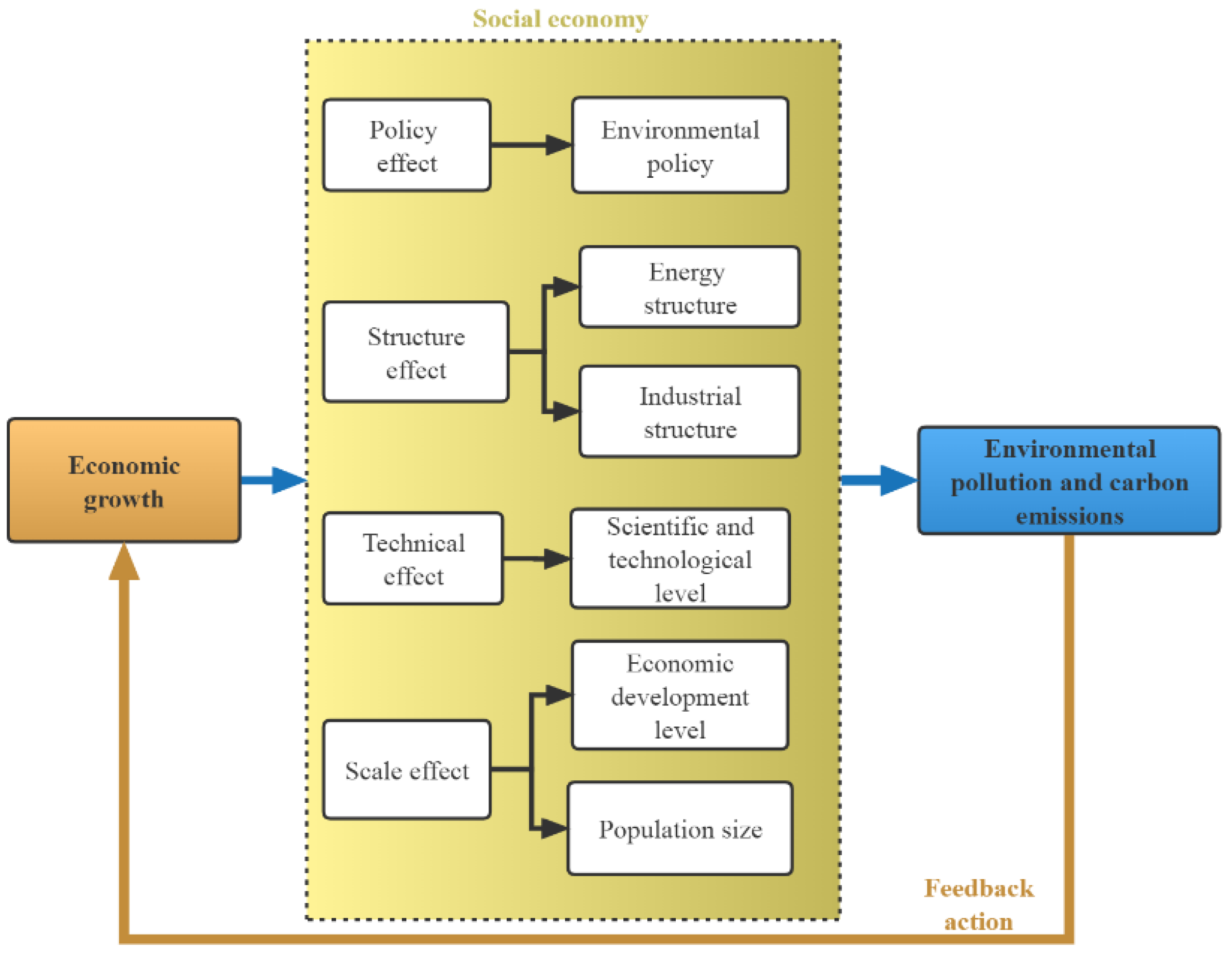
2.2. Analysis of Influencing Factors of the 3E System

With the increasingly serious greenhouse effect and environmental pollution, the analysis of carbon emission and environmental pollution has become a hot research topic. Quantitative research on carbon emission and environmental pollution is the premise to evaluate the effect of energy conservation and emission reduction [20,25]. To find out the internal driving factors of carbon emissions and environmental pollution, and to lay a foundation for the establishment of the 3E system in Fujian Province, we reviewed a large number of previous studies. All the literature can be divided roughly into three main categories: stochastic impacts by regression on population, affluence, and technology (STIRPAT) [26]; decomposition analysis; and other models. Relevant research analyzing the influencing factors of CO₂ emissions and environmental pollution is shown in

Table 1. Analysis of influencing factors of carbon emission and environmental pollution.

No.	Research	Region	Method	Carbon Emission/Environmental Pollution	Main Influencing Factors
1	[27]	China	Multivariable adjustment	environmental pollution	urban population, GDP per capita disposable income of urban residents solid waste treatment rate
2	[28]	China	STIRPAT	environmental pollution	population density energy intensity foreign direct investment
3	[29]	China	STIRPAT	environmental pollution	level of regional economic development urbanization level agricultural production
4	[30]	Asian	STIRPAT	carbon emission	urbanization, primary energy consumption, foreign direct investment
5	[31]	Europe	Index decomposition analysis	carbon emission	carbon intensity energy mix (structure) energy intensity average renewable capacity productivity change in capacity of renewable energy per capita
6	[32]	China	Computable general equilibrium model	carbon emission	energy efficiency energy structure industrial structure
7	[33]	China	Quantile regression analysis	carbon emission	GDP, energy intensity carbon intensity urbanization

.

STRIPAT, which is applied to examine the impacts of human behavior on the environment, was first proposed by Dietz and Rosa based on the Impact, Population, Affluence, and Technology model (IPAT). It is worth noting that, although the seven studies in Table 1 were carried out in different countries, objects, periods, and even models, population, economy, energy, technological progress, and policy control are considered by most scholars to be the main driving factors of carbon emissions and environmental pollution. Therefore, it can be concluded that the action mechanism of economic growth on carbon emission and environmental pollution is shown in Figure 1.

2.3. STIRPAT Model

The IPAT model is proposed to reflect the pressure of human activities on the environment.

I = P·A·T

(1)

where I refers to environmental quality, P refers to population, A refers to affluence, and T refers to technology level. However, the identity only points out the influencing factors of environmental pollution but does not indicate the influence degree of these factors. Due to the defects of IPAT mentioned above, Dietz and Rosa made some adjustments to the Equation and proposed STIRPAT (Equation (2)), which could be used for regression analysis.

I = aP^bA^cT^de

(2)

In the Equation, I, P, A, and T represent the same meanings as those in Equation (1). e denotes error; a denotes other factors that may influence environmental quality, except P, A, and T; b, c, and d denote the impacts of P, A, and T on environmental quality, respectively. To overcome the heteroscedasticity and non-normality of Equation (2), logarithms of both sides of Equation (2) are usually taken (Equation (3)).

$$\mathrm{lnI}=\mathrm{A}+\mathrm{lnP}+\mathrm{clnA}+\mathrm{dlnT}+\mathrm{e}$$

(3)

In this paper, representative pollutants carbon dioxide (carbon emission), sulfur dioxide (air pollution), chemical oxygen demand (water pollution), and solid waste (solid waste pollution) were selected as I indicators, and the indicators of the social economy in Figure 1 were selected as P, A, and T indicators. The specific variable categories and names of representative variables are shown in

Table 2. Variable and data source.

Variable Category	Variable Name	Unit	Data Source (2004–2021)
Water pollution	Chemical oxygen demand discharge (COD)	Ten thousand tons	Statistical Yearbook of Fujian Province
Atmospheric pollution	Sulfur dioxide emission (SO2)	Ten thousand tons	Statistical Yearbook of Fujian Province
Carbon emissions	Carbon dioxide emission (CO2)	Ten thousand tons	Calculated indirectly from the China Carbon Accounting Database
Solid waste pollution	Industrial solid waste discharge (ISW)	Ten thousand tons	Statistical Yearbook of Fujian Province
Economic development level	GDP per capita	CNY	Calculated indirectly by Fujian Statistical Yearbook
Population size	Population density (PD)	People/km2	Calculated indirectly by Fujian Statistical Yearbook
	Urbanization level (UL)	%	Calculated indirectly by Fujian Statistical Yearbook
Scientific and technological level	R&D expenditure/GDP (TS)	%	Statistical Yearbook of Fujian Province
Economic structure	The GDP share of secondary Industry (IS)	%	Calculated indirectly by Fujian Statistical Yearbook
	The output value of tertiary industry/output value of secondary industry (IU)	%	Calculated indirectly by Fujian Statistical Yearbook
Energy structure	Energy intensity (EI)	Tons of standard coal/CNY ten thousand	Calculated indirectly by Fujian Statistical Yearbook
	Fossil energy consumption ratio (CER)	%	Calculated indirectly by Fujian Statistical Yearbook
Environment policy	Investment in environmental practices Pollution control/GDP (IPI)	%	China Environmental Protection Database

.

2.4. Introduction to 3E System Construction in Fujian Province

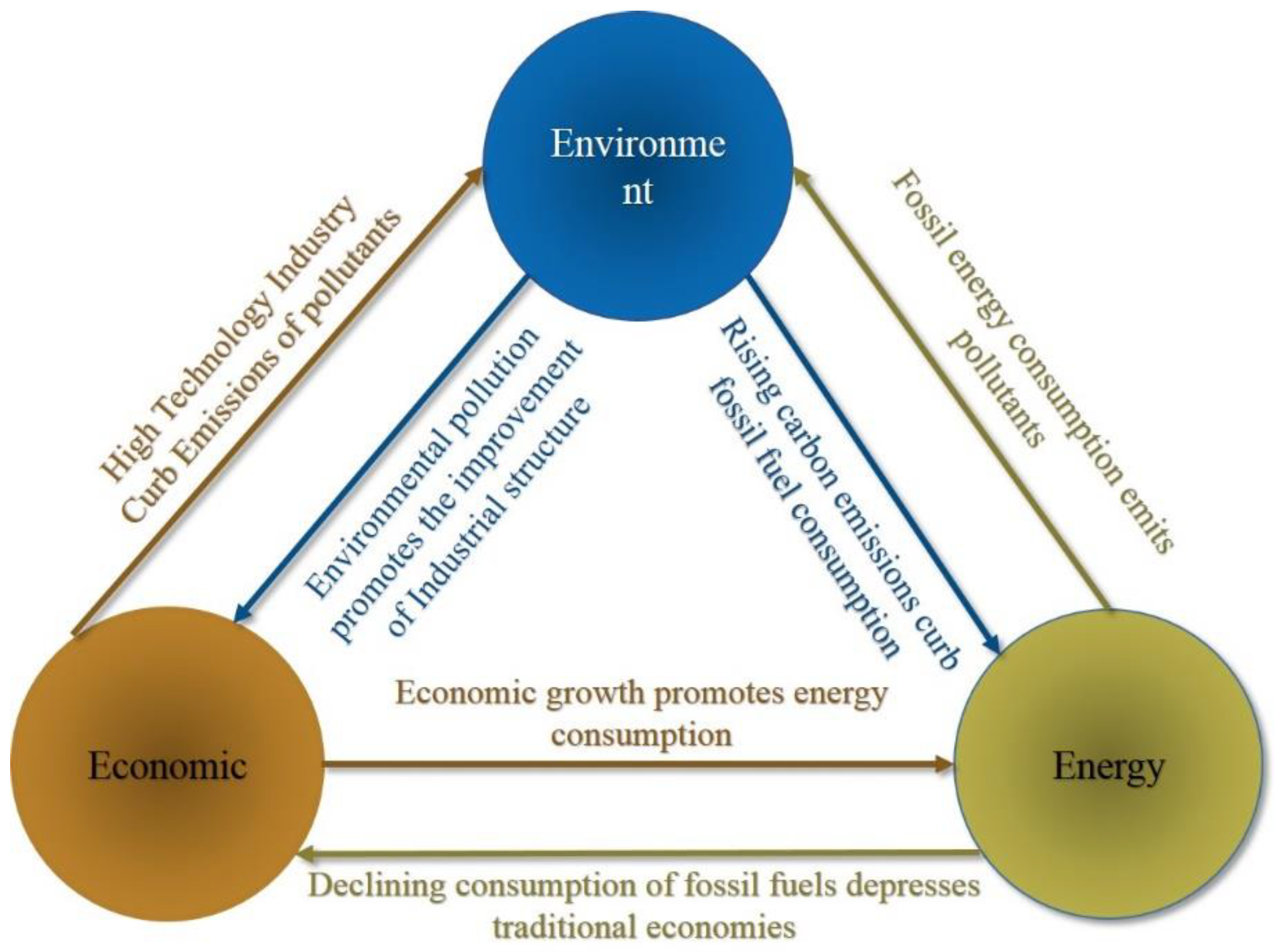
2.4.1. System Causality Description

The final research goal of this paper is the control of carbon emissions and environmental pollution in Fujian Province, which are inseparable from human activities. According to the analysis of influencing factors of carbon emission and environmental pollution in Fujian Province in Section 2.3, the influencing factors mainly focus on the industrial structure, population, and energy structure. In general, it is necessary to adjust the unreasonable energy structure and industrial structure of Fujian Province, so there is a triangular relationship between Fujian Province’s 3E systems.

(1)

Energy

From the perspective of energy, the consumption of fossil energy will promote an increase in carbon dioxide levels in the environment and a decline in environmental quality. To protect their survival environment, human beings must limit their consumption of fossil energy, that is, adjust the energy structure.

(2)

Economy

The above-mentioned adjustment of the energy structure for human beings to protect their living environment indirectly leads to a decline in traditional industries that consume a large amount of fossil energy. High-quality economic development will curb pollution emissions, and environmental pollution will also encourage people to develop high-tech industries to curb environmental pollution emissions.

(3)

Environment

From the point of view of the environment itself, no matter how it develops, there will always be polluting substances, but also a need to carry out terminal treatment to reduce the discharge of environmental pollutants.

This paper focuses on the process of pollution inhibition in causality (Figure 2).

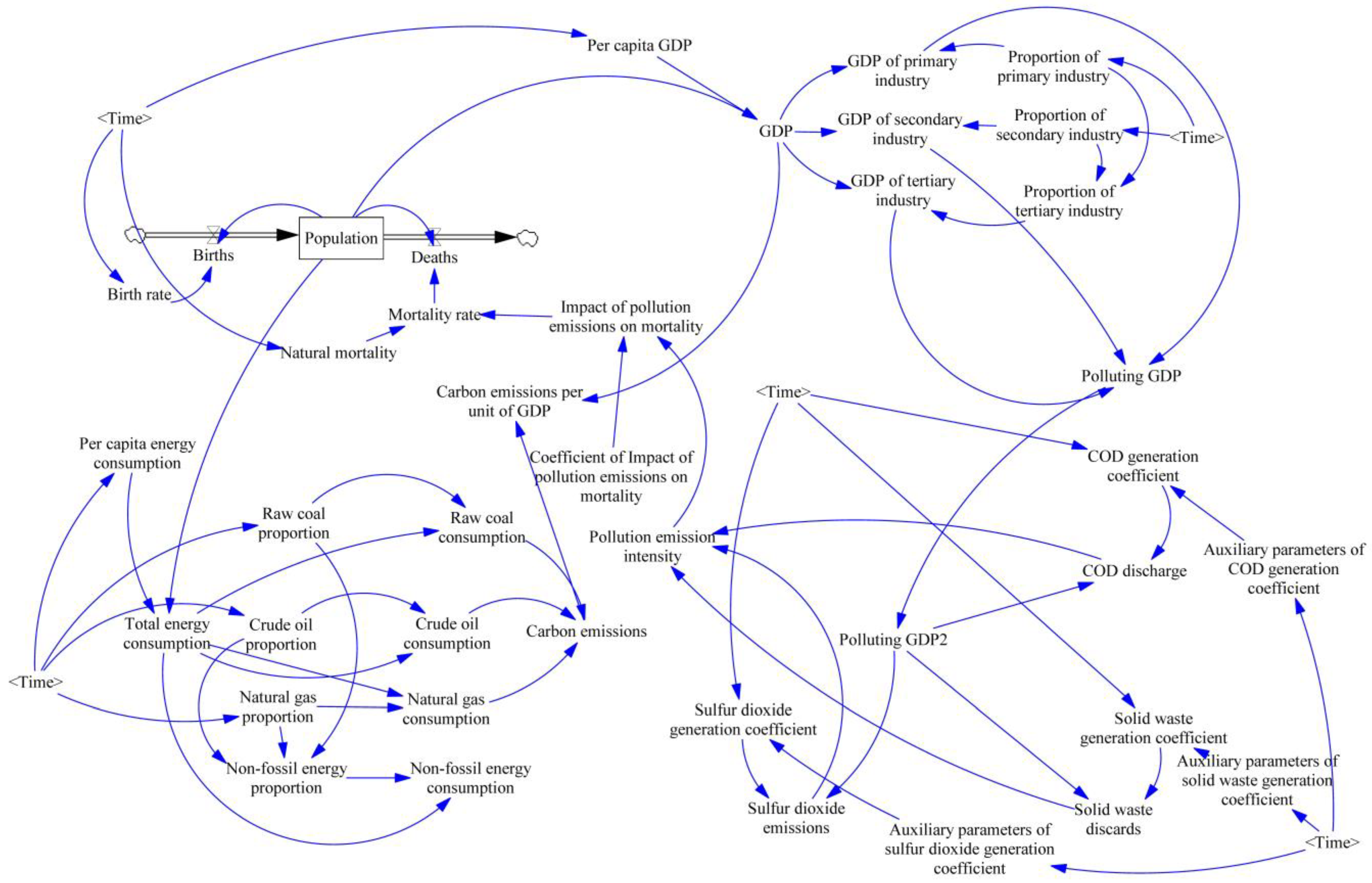
2.4.2. Model Introduction

The 3E system model in Fujian Province consists of five subsystems, namely, the population subsystem, economic subsystem, environmental pollution subsystem, energy subsystem, and carbon emission subsystem. See Figure 3 for the model diagram. See Appendix A for model related equations.

Figure 3 shows the internal relationships among subsystems of the Fujian 3E system model constructed in this paper as follows:

(1)

Population—economy and energy

The system takes population as the original driving force and links the population subsystem with the economic and energy subsystems through two indexes of per capita GDP and per capita energy consumption.

(2)

Economy—environmental pollution

In the actual production process, not all industrial activities will cause environmental pollution, so the concept of “polluting GDP” is proposed to describe the part of the economic output that will produce pollution.

There are always some activities in primary, secondary, and tertiary industries that emit significant pollutants, and the corresponding GDP is called “pollution GDP”. In the process of model operation, environmental pollution is controlled at the source by adjusting the proportion of primary, secondary, and tertiary industries in the overall GDP, to gradually reduce the proportion of the secondary industry and increase the proportion of the tertiary industry to ensure economic growth and control pollution emissions [34]. The specific expression of polluting GDP is shown in Equation (4):

PGDP = α₁·GDP1 + α₂·GDP2 + α₃·GDP3

(4)

In Equation (4), PGDP, GDP1, GDP2, and GDP3 represent the GDP of pollution production, primary industry, secondary industry, and tertiary industry, respectively. α₁, α₂, and α₃ represent the pollution production coefficients of the primary industry, secondary industry, and tertiary industry, respectively. Values of alpha1, alpha2, and alpha3 are 0.1, 0.9, and 0.1, respectively, according to the relevant literature [35]. The “pollution generation coefficient” is used to link the pollution GDP with the final pollution emissions. The “pollution generation coefficient” reflects the effect of back-end pollution treatment technology on final pollutant discharge, and the intensity of the back-end pollution reduction of a single environmental factor is regulated by this proportional coefficient. [36]

The contribution of “COD, sulfur dioxide, and solid waste” to pollution emission intensity was obtained using the entropy method.

(3)

Energy—carbon emissions

According to the total amount of energy consumption and the proportion of different types of energy, different energy consumption can be obtained. According to the carbon emission accounting method in Equation (5) and the carbon emission factors in

Table 3. Carbon emission factors of various energy sources.

Types of Energy	Carbon Emission Factors (CO2/Types of Energy)
The raw coal	0.499 t/t
Crude oil	0.838 t/t
Natural gas	0.590 t/k m3

, the carbon emissions can be obtained.

$$\mathrm{C}={{\displaystyle \sum }}^{ }{\mathrm{C}}_{\mathrm{I}}={{\displaystyle \sum }}^{ }{\mathrm{EK}}_{\mathrm{I}}\times ={\mathrm{Q}}_{\mathrm{i}}$$

(5)

In Equation (5), C denotes the total carbon emissions (MT), Ci denotes the carbon emissions of different fuels, EKi denotes the carbon emission factor of different fuels (Table 3), and Qi denotes the consumption of different fuels.

The carbon emission factors in this paper are based on the research results of Liu et al. [37] in 2015. They evaluated the emission factors of 100 typical coal mines in China, which is more suitable for China’s national conditions compared with the commonly used IPCC methods.

(4)

Environmental pollution—population

Through the influence coefficient of pollution emission on mortality, the feedback of environmental pollution to the population is realized and the system is a closed loop.

In the real world, the areas with serious environmental pollution have a high mortality rate due to environmental pollution. Therefore, the influence coefficient of environmental pollution on death was set in this model to represent the impact of environmental pollution on the death rate. The specific parameters refer to the coefficient adopted in the study of Qin of Harbin Institute of Technology [38]. However, considering that the environmental quality of Fujian Province ranks at the top in China, Qin’s coefficient is appropriately reduced in this paper.

2.4.3. Determination Method of Model Variable Equation

The data processing methods in this paper are divided into three categories: The first category is if the fitting law of variables in which time is very obvious, the change in variables in each year can be described through the linear or nonlinear fitting, and the development trend of different variables (per capita GDP, per capita energy consumption) can be obtained through the curve fitting of Origin software. The second is to use the entropy method to assign value to environmental pollution intensity. The third type is directly assigned parameters. Some parameters have no obvious change rule over time and no obvious change rule between them and other parameters. Therefore, the lookup function of the Vensim software was used to assign values directly.

2.5. Scenario Settings

This section will introduce the scenarios set up in this paper. The basis for setting scenarios mainly refers to the provisions of relevant indicators in “the 14th Five-Year Plan for National Economic and Social Development of Fujian Province and the Outline of long-term Goals in 2035” (hereinafter referred to as the “Outline”) and “the 14th Five-Year Special Plan for Ecological and Environmental Protection of Fujian Province” (hereinafter referred to as the “Plan”).

Three scenarios were set up in this paper, namely, scenarios 1, 2, and 3, and the environmental protection controls and carbon emission controls change from broad to strict.

The starting year of the model is 2003. To observe the carbon peak for 2030, the model simulates the final time of 2035, but the target year is 2030.

2.5.1. Introduction to Scenario 1

The purpose of setting up scenario 1 is mainly to investigate whether Fujian Province can achieve a carbon peak and pollutant reduction under the current development trend.

(1)

Introduction to economic structure setting

The economic structure in scenario 1 was set according to column 1 on page 12 of the “Outline”: The main indicators of economic and social development in Fujian Province during the 14th Five-Year Plan period, the proportion of regional GDP growth, and added value of the tertiary industry. Column 1 of the “Outline” set the annual GDP growth rate at 6.3%. Column 1 of the “Outline” set the annual GDP growth rate at 6.3%. The proportion of the added value of the service sector in column 1 of the “Outline” was set at more than 50% for 2025, and 2.5% growth every five years, which means that the proportion of the added value of the service sector for 2035 is 55%. Therefore, scenario 1 assumes that the proportion of the added value of the tertiary industry will increase by 2.5% every five years, and that the proportion of the primary industry will decrease to 5% in 2035.

The proportion of primary, secondary, and tertiary industries in 2035 was calculated as follows:

$${\mathrm{PTI}}_{2035}=\frac{{\mathrm{THI} \mathrm{GDP}}_{2019}+\left({\mathrm{GDP}}_{2019}\times {1.063}^{15}-{\mathrm{GDP}}_{2019}\right)\times 0.55}{{\mathrm{GDP}}_{2019}\times {1.063}^{15}}$$

(6)

PTI represents the proportion of GDP of the tertiary industry in the total GDP, and THI GDP represents the GDP of the tertiary industry.

According to the above description, the proportion of primary, secondary, and tertiary industries can be obtained, and the corresponding values for 2035 are 5%, 43.4%, and 51.6%. It was assumed that the three industries decreased or increased linearly from 2019 to obtain the values of the intermediate years.

(2)

Introduction of per capita GDP

Per capita GDP was determined through a fitting curve, and the specific equation is shown in the model equation.

(3)

Introduction of pollution generation coefficient

In scenario 1, the pollution generation coefficient of solid waste and SO₂ follows the values of 2019 to observe the emission trend of various pollutants with the development of the economy under the current pollution control efficiency.

(4)

Introduction of per capita energy consumption

Per capita energy consumption was determined through a fitting curve, and the specific equation is shown in the model equation.

(5)

Introduction of energy consumption structure

According to Table 2 of the “Plan”, the proportion of non-fossil energy in energy consumption will increase from 23.4% in 2020 to 26.1% in 2025, a cumulative increase of 2.7% in five years. The corresponding reduction in the share of fossil energy was calculated using the following Equation.

$${\mathrm{PFER}}_{\mathrm{i}, 2035}=\frac{{\mathrm{PFE}}_{\mathrm{i}, 2019}}{{\mathrm{PTFE}}_{2019}}\times {\mathrm{PNFEI}}_{2035}$$

(7)

PFER_{i, 2035} represents the proportion of fossil energy reduction in 2035 of class I, PFE_{i. 2019} represents the proportion of fossil energy in 2019 of class I, PTFE₂₀₁₉ represents the proportion of total fossil energy in 2019, and PNFEI₂₀₃₅ represents the proportion of non-fossil energy increase in 2035.

Assume that the proportion of each type of energy consumption will increase or decrease linearly between 2019 and 2035.

2.5.2. Introduction to Scenario 2

The purpose of setting scenario 2 is to investigate whether Fujian Province can achieve carbon peak and pollutant reduction under the development scenario of medium carbon emission and environmental pollution control.

(1)

Introduction to economic structure setting

The industrial structure of scenario 2 is based on the 10% (5% × 110% = 5.5%) increase in the proportion of the added value of the tertiary industry in scenario 1.

The proportion of the tertiary industry was also calculated by using Equation (5). Other assumptions are consistent with scenario 1.

(2)

Introduction of per capita GDP

Per capita GDP is the same as in scenario 1.

(3)

Introduction of pollution generation coefficient

Starting from 2019, the ratio of COD generation coefficient and solid waste generation coefficient will be 95% of that of the previous year. Starting from 2019, the ratio of SO₂ generation coefficient will be 90% of that of the previous year.

(4)

Introduction of per capita energy consumption

Per capita energy consumption from 2003 to 2019 was determined by using the fitting curve in scenario 1, and after 2019 was calculated by using Equation (8).

$${\mathrm{PCEC}}_{\mathrm{i}}={\mathrm{PCEC}}_{2019}+\left(\mathrm{time}-2019\right)\times \mathrm{EXP}\left(-0.00125\times \mathrm{time}\right)$$

(8)

PCEC_i represents per capita energy consumption for the year I, and PCEC₂₀₁₉ represents per capita energy consumption for the year 2019.

Currently, the per capita energy consumption in most developed countries has reached its peak and started to decline, and China is still in the period of rising per capita energy consumption [39]. The proposed purpose of Equation (8) is to increase the per capita energy consumption of Fujian Province to approximately 80% of Germany’s per capita energy consumption in 2019 (5.4 tons per year) by 2030, and gradually reduce the growth rate of per capita energy consumption in Fujian when the per capita energy consumption increases, and finally, when the per capita energy consumption becomes stable, to implement the policy of reducing per capita energy consumption in the future.

(5)

Introduction of energy consumption structure

The energy consumption structure in scenario 2 increases by 10% (2.7% × 110% = 2.97%) on the basis of scenario 1 (2.7%). In other words, the accumulative growth was 2.97% in 5 years and 8.91% in 15 years. The calculation method of various energy ratios is the same as in Equation (7).

2.5.3. Introduction to Scenario 3

The purpose of scenario 3 is to investigate whether Fujian Province can achieve carbon peak and pollutant reduction under the development scenario of strict control of carbon emission and environmental pollution.

(1)

Introduction to industrial structure

The industrial structure of scenario 3 is based on the proportion of added value of the tertiary industry in scenario 1 (5%), which increased by 20% (5% × 120% = 6%). In other words, the accumulative growth was 6% in 5 years and 18% in 15 years The proportion of the tertiary industry was also calculated by using Equation (5). Other assumptions are consistent with scenario 1.

(2)

Introduction of per capita GDP

GDP per capita is the same as in scenario 1.

(3)

Introduction of pollution generation coefficient

Starting from 2019, the ratio of COD generation coefficient and solid waste generation coefficient will be 90% of that of the previous year. Starting from 2019, the ratio of SO₂ generation coefficient will be 85% of that of the previous year.

(4)

Introduction of per capita energy consumption

Per capita energy consumption from 2003 to 2019 was determined by using the fitting curve in scenario 1, and after 2019 was calculated by using Equation (9).

$${\mathrm{PCEC}}_{\mathrm{i}}={\mathrm{PCEC}}_{2019}+\left(\mathrm{time}-2019\right)\times \mathrm{EXP}\left(-0.002\times \mathrm{time}\right)$$

(9)

PCEC_i represents per capita energy consumption for the year I, and PCEC₂₀₁₉ represents per capita energy consumption for the year 2019.

The proposed purpose of Equation (9) is to increase the per capita energy consumption of Fujian Province to approximately 80% of Japan’s per capita energy consumption in 2019 (5.0 tons per year) by 2030, and gradually reduce the growth rate of per capita energy consumption in Fujian when the per capita energy consumption increases, and when the per capita energy consumption finally becomes stable, to implement the policy of reducing per capita energy consumption in the future.

(5)

Introduction of energy consumption structure

The energy consumption structure in scenario 2 increases by 30% (2.7% × 130% = 3.51%) on the basis of scenario 1 (2.7%); that is, the accumulative growth of five years was 3.51%, and the accumulative growth of 15 years was 10.053%. The calculation method of various energy ratios is the same as in Equation (7).

2.6. Description of Controlling Objectives for the Target Year (2030)

This model focuses on the emissions of pollutants, so the control targets are divided into carbon emissions, COD discharge, solid waste discards, and SO₂ emissions.

Carbon emissions are mainly concerned with whether there will be a “carbon peak” before 2030, that is, whether there will be a historical peak of carbon dioxide emissions in one year before 2030 and no rebound trend of carbon emissions in the following years.

COD discharges, solid waste discards, and SO₂ emissions in the target year were set according to the actual completion of pollution emission reduction targets in Table 1 in the “Plan” during the 13th Five-Year Plan period. During the 13th Five-Year Plan period, COD discharges decreased by 4.5%, so 2030 is set to decrease by 8.9% compared with 2019, and the calculation method is shown in Equation (10). The value of solid waste discards was set as 8.9%, and the calculation method is shown in Equation (10). According to Table 1 in the “Plan”, SO₂ emissions decreased by 29.5% during the 13th Five-Year Plan period, so the value for 2030 was set as 51% lower than that in 2019, and the calculation method is shown in Equation (10).

$${\mathrm{IDV}}_{\mathrm{i},2030}=1-{\mathrm{IPV}}_{\mathrm{i},2019}\times \left(1-{\mathrm{IDV}}_{13\mathrm{th}}^2\right)$$

(10)

${\mathrm{IDV}}_{\mathrm{i},2030}$ represents a decrease value in 2030 of index I, ${ \mathrm{IPV}}_{\mathrm{i},2019}$ represents the pollution value in 2030 of index I, and IDV_13th represents a decrease value in the 13th Five-Year Plan period of index I.

3. Results and Discussion

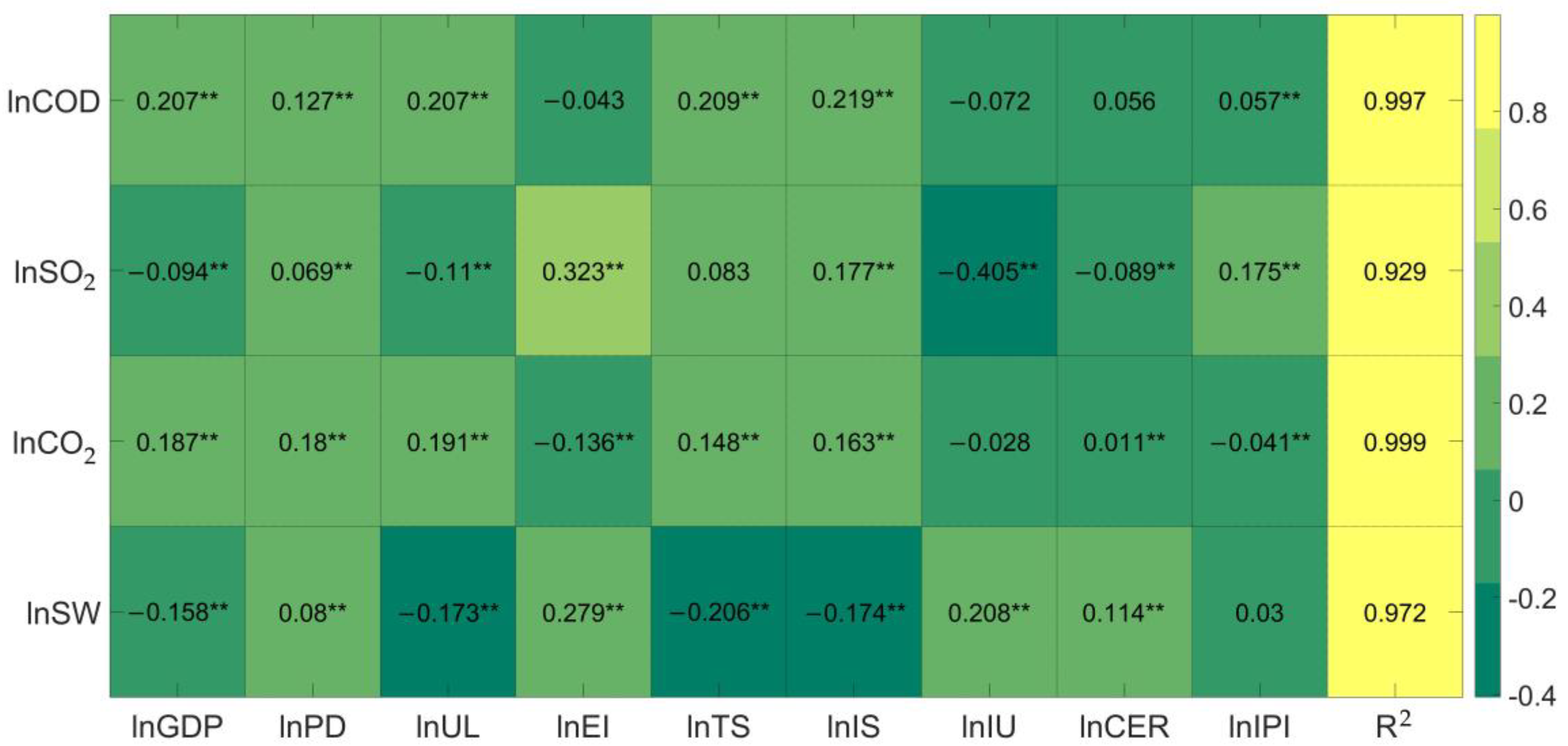
3.1. STIRPAT Model

In this paper, lnCOD, lnSO₂, lnCO₂, and lnSW in Fujian Province are defined as dependent variable I. lnGDP, lnPD, lnUL, lnEI, lnTS, lnIS, lnIU, lnCER, and lnIPI are defined as independent variable PAT. Regression results are shown in Figure 4.

It can be seen that the R² of all four groups of equations is greater than 0.929, indicating that the regression results are credible. According to Figure 4, the four indexes with the greatest impact on water pollution, air pollution, carbon emission, and solid waste pollution in Fujian Province are as follows: IS (0.21898), IU (−0.40498), UL (0.19062), and EI (0.27874) are the same as the conclusions of He, Li, and Wang et al. [28,29,40].

IS, IU, UL, and EI belong to the three variable categories of economic structure, population size, and energy structure, respectively, in Table 2. Therefore, the modeling idea of the Fujian Province 3E system in this paper can take the population as the most original driving force and use per capita GDP and per capita energy consumption to connect the population subsystem with the energy and economic subsystem. Use the industrial structure and energy structure adjustment to achieve environmental pollution and carbon dioxide control.

3.2. Fujian Province 3E System Model

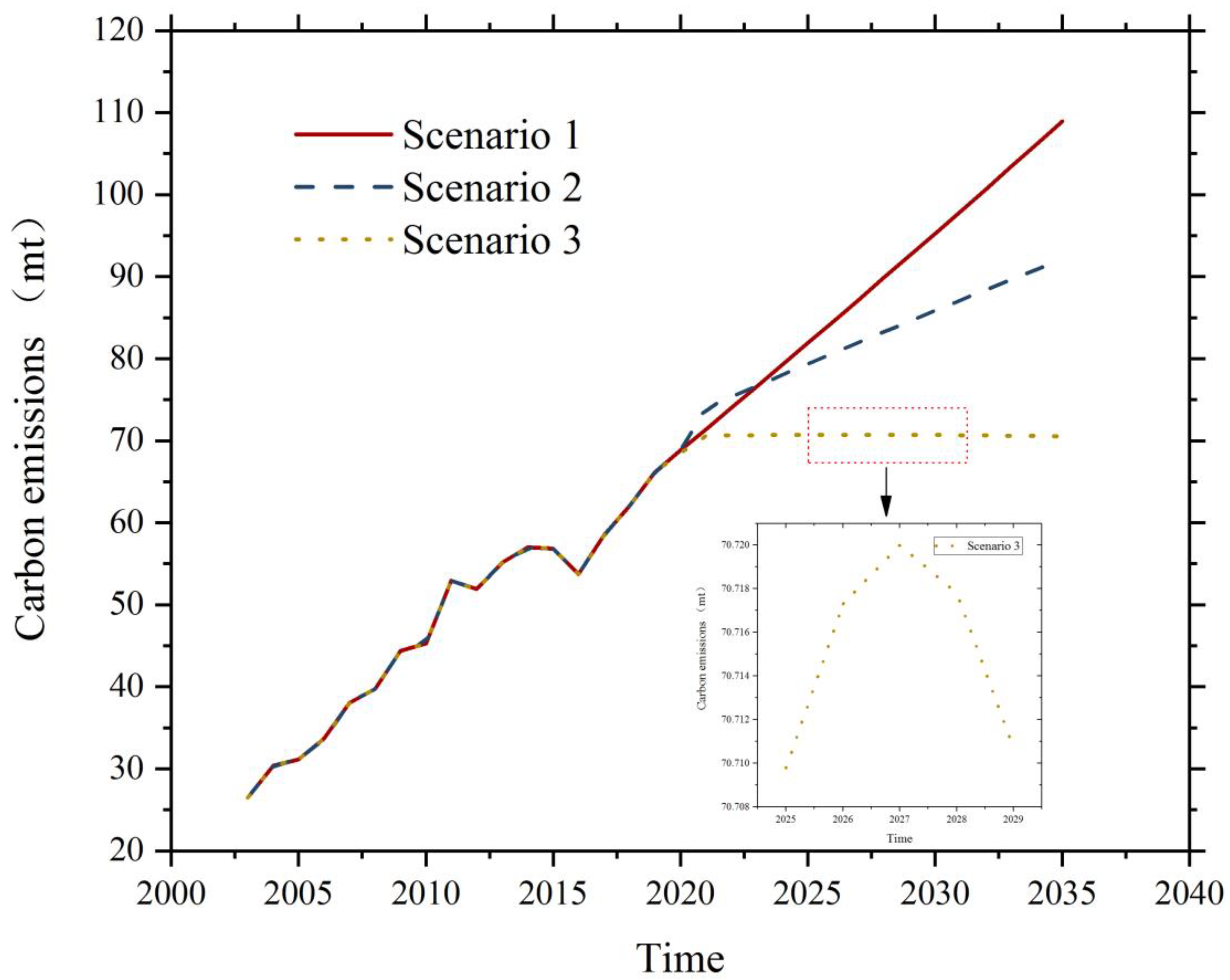
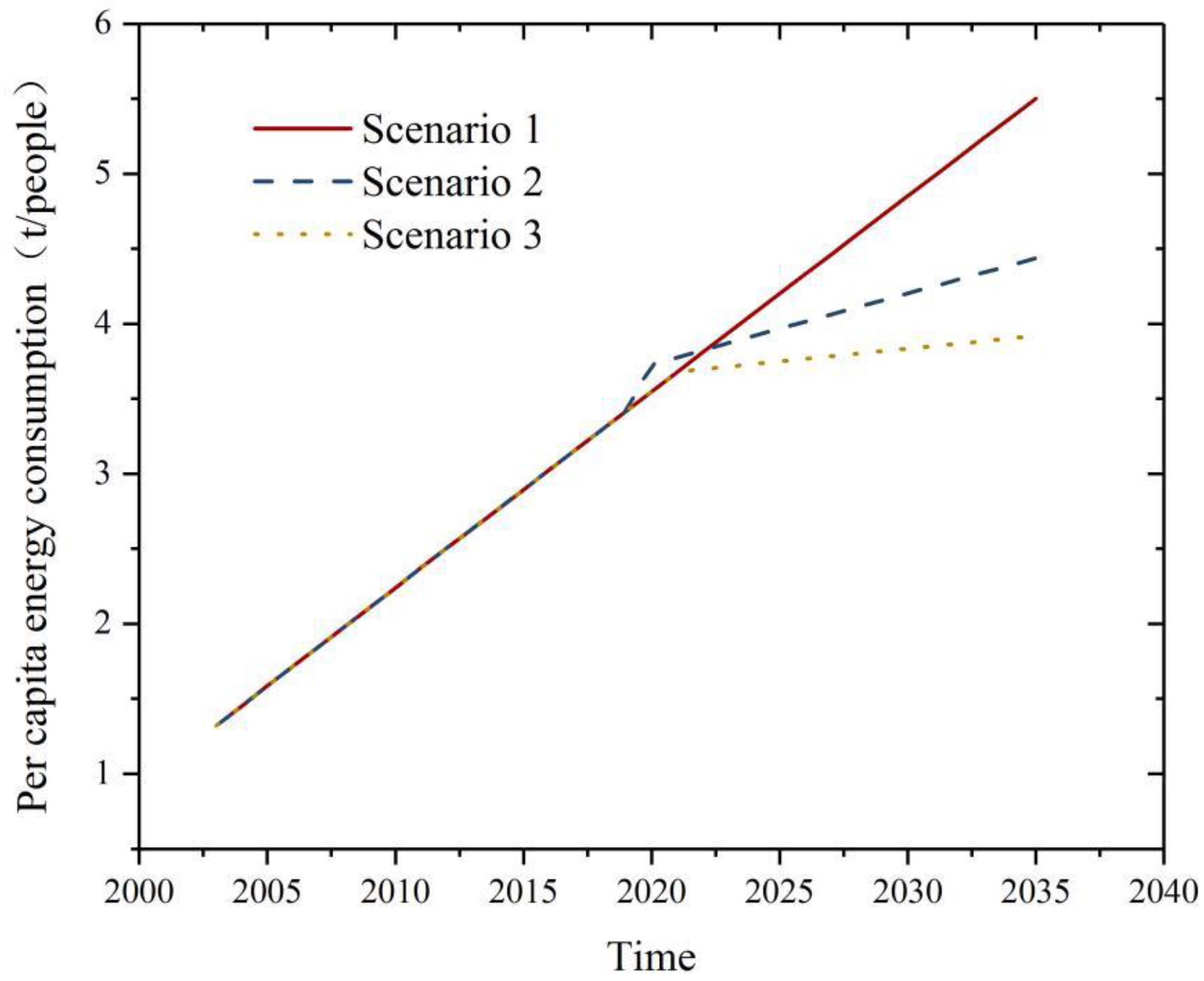
3.2.1. Scenario Simulation of per Capita Energy Consumption and Carbon Emission in Fujian Province

It can be seen from Figure 5 that per capita energy consumption in Fujian Province presents a rising trend under three scenarios, with an increasing rate from large to small, respectively: scenario one, scenario two, and scenario three. It shows that under the three development scenarios, people’s living standards can be guaranteed, and there will not be a decline in the quality of life caused by the decrease in per capita energy consumption due to policy reasons [41].

As can be seen from Figure 6, the carbon emission of Fujian Province rises sharply under scenario one, which indicates that the continuous development of Fujian Province under the current development trend cannot reach the carbon peak in 2030 as scheduled. The main reason lies in the rapid increase in per capita energy consumption and irrational energy structure.

In the development scenario of scenario two, Fujian Province does not achieve the carbon peak in 2030 as scheduled, and the carbon emission of Fujian Province will surpass that of scenario one briefly during the period 2020–2023. After 2023, the carbon emission of Fujian Province in scenario two is less than that in scenario one, and the gap between them gradually widens. This is because the setting of Equation (8) makes the per capita energy consumption of scenario two larger than that of scenario one during the period 2020–2023. Over time, the per capita energy consumption growth of Scenario two decreases year by year, and the impact of energy structure adjustment on carbon emissions also begins to appear.

In the development scenario of scenario three, carbon emissions in Fujian Province will rise gradually from 2020 to 2027, and then gradually decline after reaching 70.72 mt in 2027, indicating that under the development mode of per capita energy consumption and energy structure in scenario three, Fujian Province can achieve carbon peak on schedule. However, the relatively weak “peak” is not conducive to the subsequent carbon neutralization process.

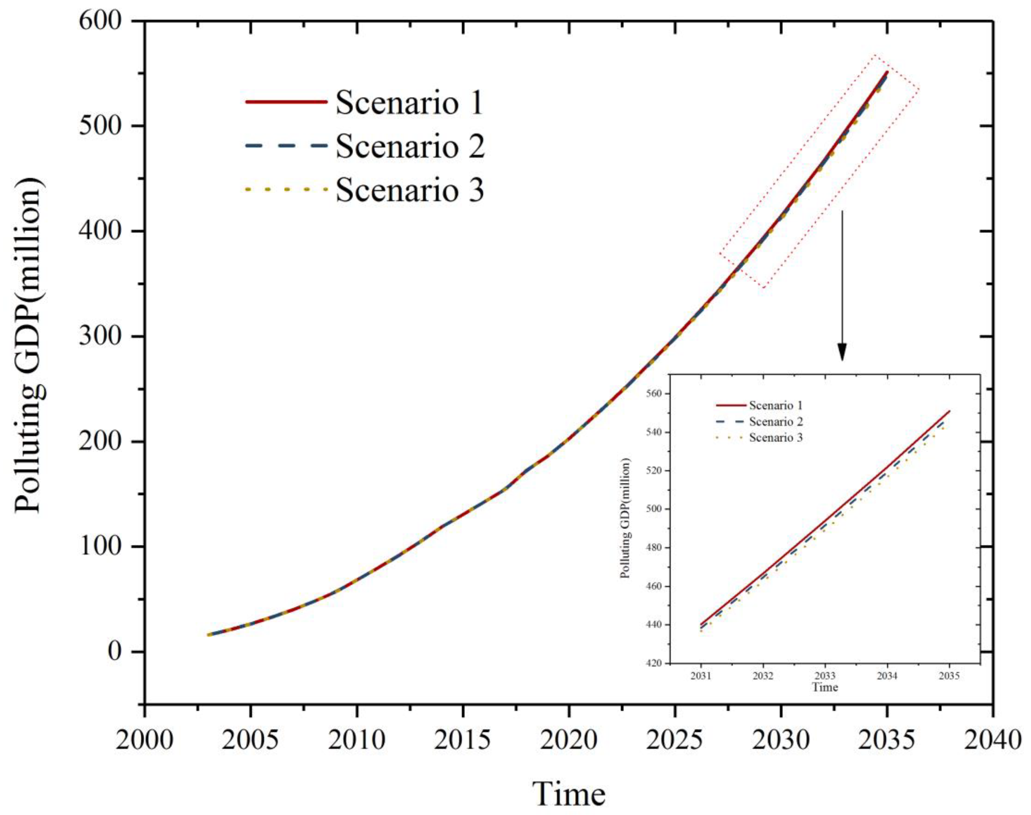
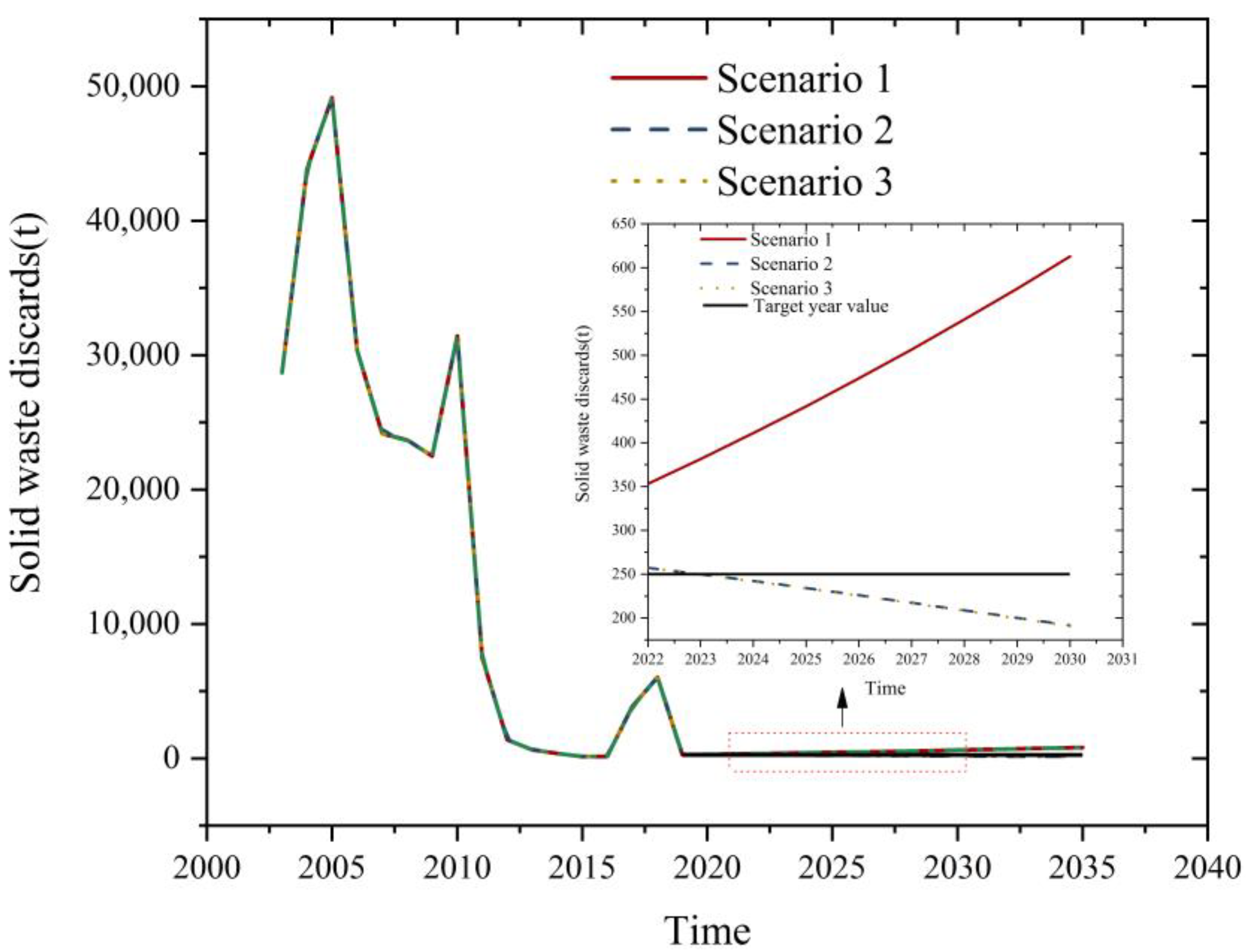
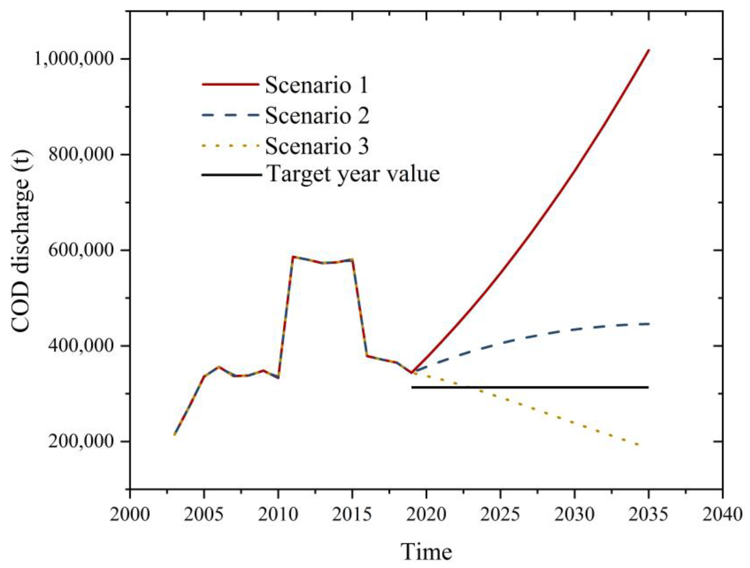
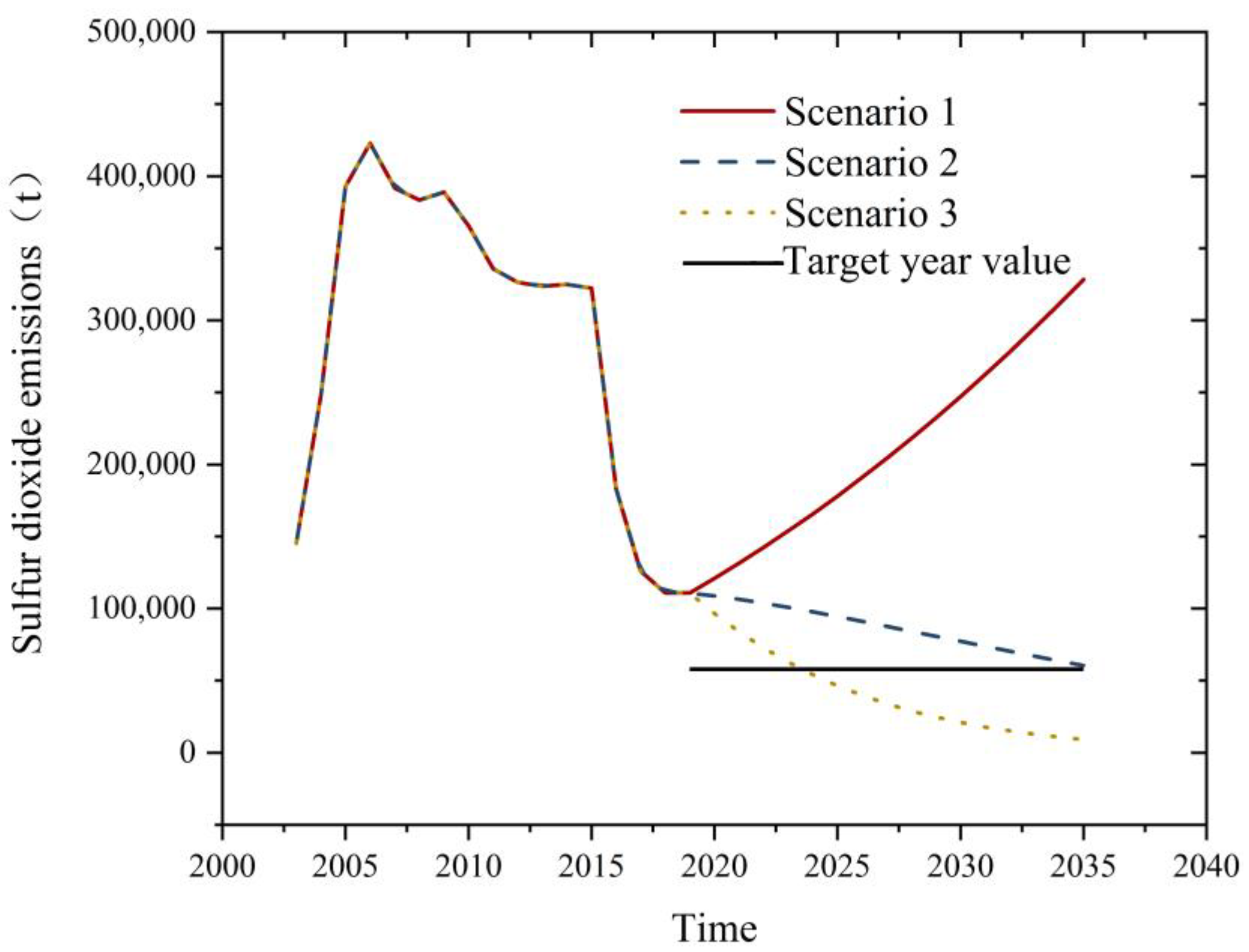
3.2.2. Environmental Pollution Scenario Simulation in Fujian Province

As can be seen from Figure 7, under the current economic growth rate, the polluting GDP of Fujian Province is rising rapidly under the three scenarios. This is because the per capita GDP of Fujian Province is still developing, and the adjustment of the industrial structure is not enough to reduce pollution at the front end.

As can be seen from the partially enlarged Figure 7, the numerical gap between the polluting GDP of the three scenarios gradually increases over time. Development scenario one has the highest value, scenario two has the middle value, and scenario three has the lowest value. This is due to the development mode of scenario one, which has the unhealthiest economic structure and the highest proportion of the secondary industry. This shows that the adjustment of the industrial structure can control pollution at the source, but it is not enough to reduce environmental pollution, and the end treatment technology is still an important way to reduce environmental pollution in the current development stage.

As can be seen from Figure 8, under the development mode of scenario one, water pollution substances in Fujian Province are rising rapidly. This is because the economic structure of scenario one is unreasonable and the pollution generation coefficient of the water environmental factors adopts the value of 2019 and does not attenuate over time, that is, the terminal treatment technology of pollutants does not improve over time. The growth rate of water pollutant discharge in Fujian Province is positive from 2019 to 2035 and gradually decreases with the passage of time. This indicates that with the passage of time, the industrial structure adjustment at the source and pollutant treatment measures at the back end of scenario two gradually reduce the water pollution in Fujian Province. Under scenario three development mode, the water pollutants in Fujian Province reach the target annual value in advance in 2024. This indicates that the industrial structure at the source and pollutant treatment technology at the end of scenario three play an important role in pollutant reduction.

As can be seen from Figure 9, under the development mode of scenario one, air pollution substances in Fujian Province are rising rapidly. This is because the economic structure of scenario one is unreasonable and the pollution generation coefficient of the air environmental factors adopts the value of 2019 and does not attenuate over time, that is, the terminal treatment technology of pollutants does not improve over time. In scenario two, the emissions of air pollutants in Fujian Province show a decreasing trend year by year from 2019 to 2035 but fail to reach the target annual value in 2030. This is because the target annual reduction ratio of air pollutants is larger than that of water pollutants and solid waste. Therefore, the economic structure of scenario two is insufficient to achieve pollutant reduction at the source. Under the scenario three development mode, the air pollutants in Fujian Province reach the target annual value in advance in 2024. This indicates that the industrial structure at the source and pollutant treatment technology at the end of scenario three play an important role in pollutant reduction.

As can be seen from Figure 10 under the development mode of scenario one, the solid waste emissions of Fujian Province increase rapidly after 2019. The causes of this condition are consistent with those of water and atmospheric environmental factors. In scenario two and scenario three, the solid waste in Fujian Province reaches the target annual value. It is not difficult to reduce the number of solid waste discards in Fujian Province.

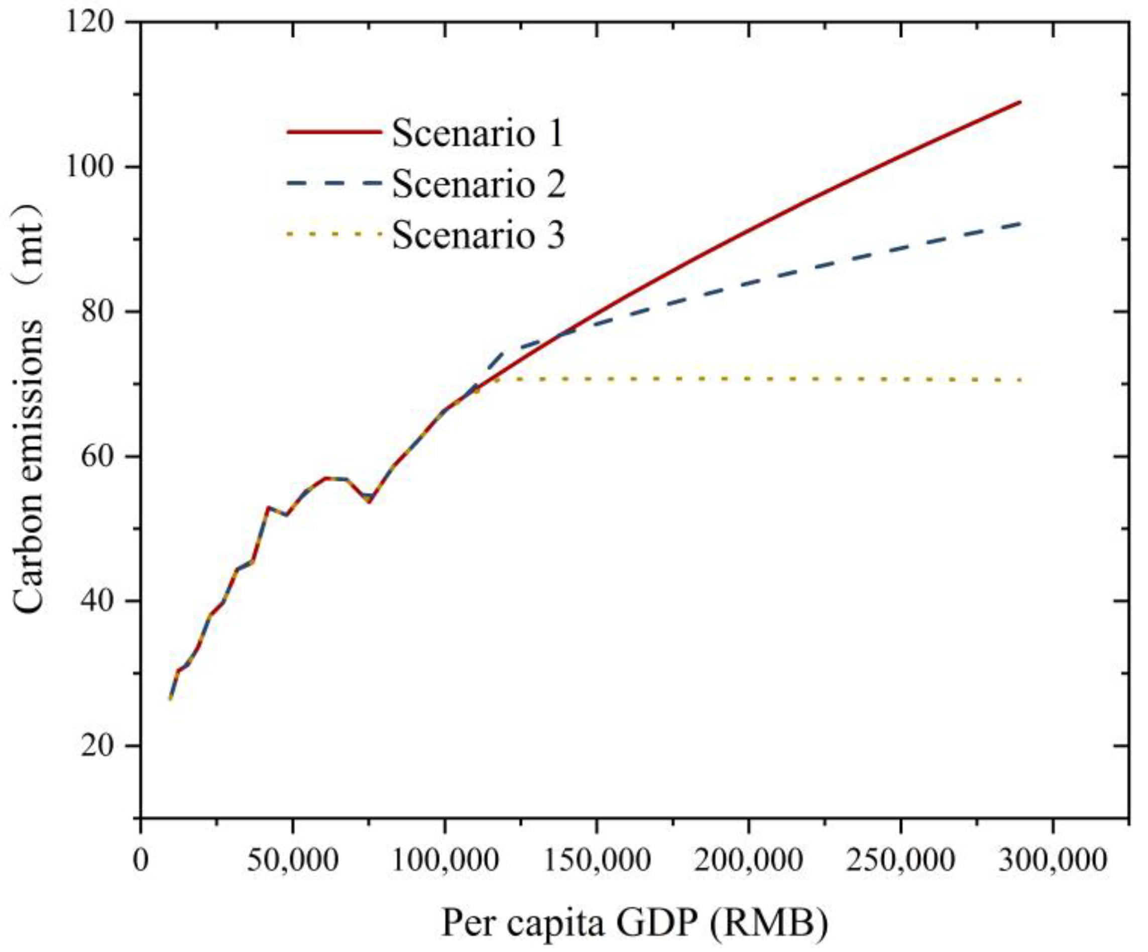
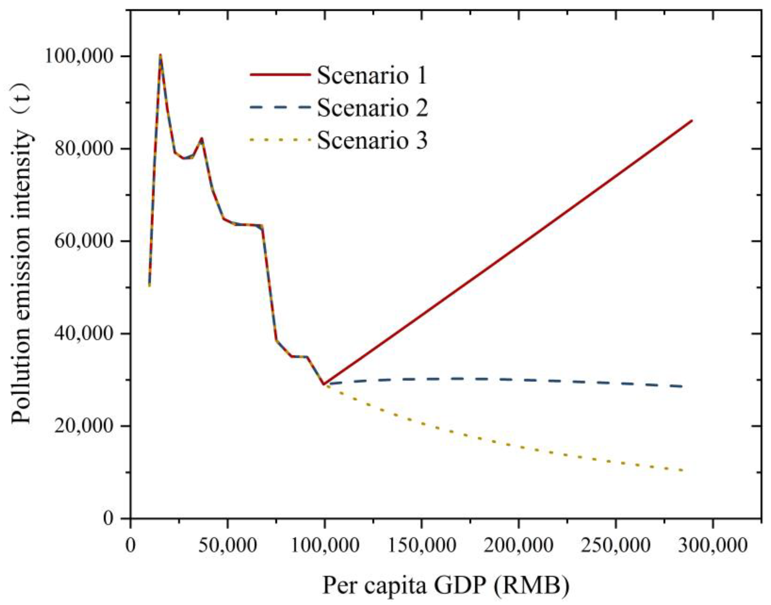
3.3. Discussion on EKC of Fujian Province

After analyzing the carbon emissions and environmental pollution emissions of Fujian Province under three scenarios, we attempted to investigate the EKC hypothesis proposed by Kuznets and defined by Panayotou [42]. The simulation accuracy of this model fits well with the trend of actual data. Therefore, the development trend of EKC in Fujian Province was observed by using simulated data directly [43].

The EKC curve describes how carbon emissions and environmental pollution begin to decline after income levels reach a certain critical point. Results of the EKC hypothesis in Fujian Province under three development scenarios are shown in Figure 11 and Figure 12. The abscissa is the predicted per capita GDP of Fujian Province in the period 2003–2035, and the ordinate is the predicted carbon emission and pollution emission intensity of Fujian Province in the period 2003–2035. The results show that there is no downward trend or “inflection point” of carbon emission in Fujian Province in scenario one and scenario two. In scenario three, when the per capita GDP of Fujian reaches RMB 181824, carbon emissions will decrease with the increase in per capita GDP.

Under the three scenarios, the first “inflection point” of pollution emission intensity in Fujian Province appears when the per capita GDP is RMB 67,648. However, the pollution emission intensity of the three development scenarios shows different trends. In the development mode of scenario one, after per capita GDP reaches RMB 99,456, and pollution emission intensity begins to rise due to environmental pollution control technology no longer making progress, the overall EKC curve shows an “N” shape, which is the same as the research results of Brajer et al. [44]. In scenario two, when the per capita GDP is between 99,456 and 232,384, the pollution emission intensity of Fujian Province rises and then begins to decline, making the overall EKC curve an “M” type, which is consistent with the conclusions of Inmaculada et al. [45]. In scenario three, the pollution emission intensity of Fujian begins to decline after per capita GDP reaches RMB 99,456, which is in line with the most common inverted “U” type.

4. Conclusions and Policy Recommendations

4.1. Conclusions

This paper first analyzed the influencing factors of environmental pollution and carbon emissions in Fujian Province using the STIRPAT model, aiming to explore the main driving factors of environmental pollution and carbon emissions in Fujian Province and provide a quantitative basis for the establishment of a subsequent system dynamics model. In addition, the 3E model of Fujian Province was established by using the system dynamics model. This model combined 3E-P and 3E-C coupling analysis to study whether Fujian can achieve a carbon peak in 2030 and achieve the reduction target of environmental pollution and the EKC hypothesis under three development scenarios. We can draw the following conclusions: (1) the main influencing factors of environmental pollution and carbon emissions in Fujian Province belong to the variable category of population, economic structure, and energy consumption structure. (2) The current development trend of Fujian Province is not sustainable, and it cannot achieve carbon peak and pollutant reduction by 2030 as scheduled. In scenario three, Fujian Province can achieve carbon peak and pollutant reduction targets on schedule. (3) There is no “inflection point” in the carbon emission EKC curve of scenarios one and two in Fujian Province. Under the development trend of scenario three, an inverted U-shaped EKC curve appears. The EKC curves of environmental pollution scenarios one and two in Fujian Province are “N” and “M”, respectively, which are different from the common inverted “U”.

4.2. Policy Recommendations

It can be seen from the above simulation results that the development trend of scenario three should be adopted to achieve a carbon peak and pollutant reduction in the target year.

Therefore, the following suggestions are proposed for the above situation:

(1)

Carbon emissions

In terms of carbon emissions, the proportion of non-fossil energy in Fujian Province is relatively low in the current planning. In 2030, the proportion of non-fossil energy should be increased by approximately 38–40%, and the per capita energy consumption can be moderately increased to 4.0 tons (the per capita energy consumption in the UK in 2019), so that there can be a relatively obvious peak trend to facilitate subsequent carbon neutrality.

(2)

Pollution discharge

In terms of pollution discharge, the reduced pressure of COD and solid waste in Fujian Province is small, but the reduced pressure of SO₂ is large. To reduce the SO₂ reduction pressure, an increase of 2.5–5% from the 50% ratio of tertiary industry in scenario three would reduce total pollution GDP by 4.5–9%.

To achieve the above goals, Fujian Province can: (1) optimize the structure of residents’ energy use by implementing energy pricing policy; (2) improve the carbon trading mechanism, optimize the efficiency of carbon trading, encourage enterprises to use clean energy, and develop clean production technology; (3) starting from the three leading industries of electronics, petrochemical, and machinery in Fujian Province, extend the upstream and downstream industry chain, and promote the development of leading industries from “low quality” and “low value” to “high quality” and “high value”.

Based on the simulation results, we proposed some policy suggestions in this section. The specific numerical suggestions are only suitable for Fujian Province. However, improving energy pricing, increasing carbon trading efficiency, and upgrading major industries are common paths for all regions with carbon and pollution emissions pressures.

References

1. Yang, H.; Li, X.; Ma, L.; Li, Z. Using system dynamics to analyse key factors influencing China’s energy-related CO2 emissions and emission reduction scenarios. J. Clean. Prod. 2021, 320, 128811. [Google Scholar] [CrossRef]
2. Roelfsema, M.; Soest, H.V.; Harmsen, M.; Vuuren, D.V.; Bertram, C.; Elzen, M.D.; Iacobuta, G.; Krey, V.; Kriegler, E.; Luderer, G. Taking stock of national climate policies to evaluate implementation of the Paris Agreement. Nat. Commun. 2020, 11, 2096. [Google Scholar] [CrossRef]
3. Zuo, Y.; Shi, Y.-l.; Zhang, Y.-z. Research on the Sustainable Development of an Economic-Energy-Environment (3E) System Based on System Dynamics (SD): A Case Study of the Beijing-Tianjin-Hebei Region in China. Sustainability 2017, 9, 1727. [Google Scholar] [CrossRef]
4. IPCC AR6 Synthesis Report: Climate Change 2022. Available online: https://www.ipcc.ch/report/sixth-assessment-report-cycle/ (accessed on 21 April 2022).
5. GOFJP Issued by Fujian Provincial People’s Government Fujian Province National Economic and Social Development of the Fourteenth Five-Year Plan and Notice on the Outline of the Vision for 2035. Available online: https://www.fujian.gov.cn/zwgk/zfxxgk/szfwj/szfgz/202103/t20210319_5552893.htm (accessed on 21 March 2021).
6. Zhang, S.; Hu, T.; Li, J.; Cheng, C.; Song, M.; Xu, B.; Baležentis, T. The effects of energy price, technology, and disaster shocks on China’s Energy-Environment-Economy system. J. Clean. Prod. 2019, 207, 204–213. [Google Scholar] [CrossRef]
7. Groncki, P.J.; Marcuse, W. Brookhaven Integrated Energy/Economy Modeling System and Its Use in Conservation Policy Analysis; Brookhaven National Lab.: Upton, NY, USA, 1982; pp. 535–555.
8. Forrest, J.W. Industrail Dynamics; MIT Press: Cambridge, MA, USA, 1964. [Google Scholar]
9. Forrest, J.W. Urban Dynamics; MIT Press: Cambridge, MA, USA, 1969. [Google Scholar]
10. Forrest, J.W. World Dynamics; Wright-Allen Press: Cambridge, MA, USA, 1971. [Google Scholar]
11. Isa, S.H.; Ramlee, M.N.A.; Lola, M.S.; Ikhwanuddin, M.; Azra, M.N.; Abdullah, M.T.; Zakaria, S.; Ibrahim, Y. A system dynamics model for analysing the eco-aquaculture system of integrated aquaculture park in Malaysia with policy recommendations. Environ. Dev. Sustain. 2021, 23, 511–533. [Google Scholar] [CrossRef]
12. Khajehpour, H.; Ahmady, M.A.; Hosseini, S.A.; Mashayekhi, A.N.; Maleki, A. Environmental policy-making for Persian Gulf oil pollution:A future study based on system dynamics modeling. Energy Sources Part B Econ. Plan. Policy 2016, 12, 17–23. [Google Scholar] [CrossRef]
13. Xiao, S.; Dong, H.; Geng, Y.; Tian, X.; Li, H. Policy impacts on Municipal Solid Waste management in Shanghai: A system dynamics model analysis. J. Clean. Prod. 2020, 262, 121366. [Google Scholar] [CrossRef]
14. Guo, X.; Ren, D.; Guo, X. A system dynamics model of China’s electric power structure adjustment with constraints of PM10 emission reduction. Environ. Sci. Pollut. Res. 2018, 25, 17540–17552. [Google Scholar] [CrossRef]
15. Dai, D.; Sun, M.; Lv, X.; Hu, J.; Zhang, H.; Xu, X.; Lei, K. Comprehensive assessment of the water environment carrying capacity based on the spatial system dynamics model, a case study of Yongding River Basin in North China. J. Clean. Prod. 2022, 344, 131137. [Google Scholar] [CrossRef]
16. Wang, G.; Xiao, C.; Qi, Z.; Meng, F.; Liang, X. Development tendency analysis for the water resource carrying capacity based on system dynamics model and the improved fuzzy comprehensive evaluation method in the Changchun city, China. Ecol. Indic. 2021, 122, 107232. [Google Scholar] [CrossRef]
17. Yang, J.; Strokal, M.; Kroeze, C.; Wang, M.; Wang, J.; Wu, Y.; Bai, Z.; Ma, L. Nutrient losses to surface waters in Hai He basin: A case study of Guanting reservoir and Baiyangdian lake. Agric. Water Manag. 2019, 213, 62–75. [Google Scholar] [CrossRef]
18. Collatto, D.C.; Lacerda, D.P.; Morandi, M.; Piran, F.S. Environmental externalities in broiler production: An analysis based on system dynamics. J. Clean. Prod. 2019, 209, 190–199. [Google Scholar]
19. Jin, E.; Mendis, G.P.; Sutherland, J.W. Integrated sustainability assessment for a bioenergy system: A system dynamics model of switchgrass for cellulosic ethanol production in the U.S. midwest. J. Clean. Prod. 2019, 234, 503–520. [Google Scholar] [CrossRef]
20. Navarro, A.; Moreno, R.; Jimenez-Alcazar, A.; Tapiador, F.J. Coupling population dynamics with earth system models: The POPEM model. Environ. Sci. Pollut. Res. Int. 2019, 26, 3184–3195. [Google Scholar] [CrossRef] [PubMed]
21. Benvenutti, L.M.; Uriona-Maldonado, M.; Campos, L. The impact of CO2 mitigation policies on light vehicle fleet in Brazil. Energy Policy 2019, 126, 370–379. [Google Scholar] [CrossRef]
22. Sun, L.; Niu, D.; Wang, K.; Xu, X. Sustainable development pathways of hydropower in China: Interdisciplinary qualitative analysis and scenario-based system dynamics quantitative modeling. J. Clean. Prod. 2020, 287, 125528. [Google Scholar] [CrossRef]
23. Watabe, A.; Leaver, J.; Ishida, H.; Shafiei, E. Impact of low emissions vehicles on reducing greenhouse gas emissions in Japan. Energy Policy 2019, 130, 227–242. [Google Scholar] [CrossRef]
24. Wang, M.; Che, Y.; Yang, K.; Wang, M.; Xiong, L.; Huang, Y. A local-scale low-carbon plan based on the STIRPAT model and the scenario method: The case of Minhang District, Shanghai, China. Energy Policy 2011, 39, 6981–6990. [Google Scholar] [CrossRef]
25. Azevedo, V.G.; Sartori, S.; Campos, L.M.S. CO2 emissions: A quantitative analysis among the BRICS nations. Renew. Sustain. Energy Rev. 2018, 81, 107–115. [Google Scholar] [CrossRef]
26. Dietz, T.; Rosa, E.A. Effects of population and affluence on CO2 emissions. Proc. Natl. Acad. Sci. USA 1997, 94, 175. [Google Scholar] [CrossRef]
27. Chu, Z.; Wu, Y.; Zhou, A.; Huang, W.C. Analysis of influence factors on municipal solid waste generation based on the multivariable adjustment. Environ. Prog. Sustain. Energy 2016, 35, 1629–1633. [Google Scholar] [CrossRef]
28. He, Y.; Lin, K.; Liao, N.; Chen, Z.; Rao, J. Exploring the spatial effects and influencing factors of PM2.5 concentration in the Yangtze River Delta Urban Agglomerations of China. Atmos. Environ. 2022, 268, 118805. [Google Scholar] [CrossRef]
29. Li, L.G.I.; Zhang, P.Y.; Liu, W.X.; Jing, L.I.; Wang, L.F. Spatial-temporal evolution characteristics and influencing factors of county-scale environmental pollution in Jilin Province, Northeast China. Chin. J. Appl. Ecol. 2019, 30, 2361–2370. [Google Scholar]
30. Behera, S.R.; Dash, D.P. The effect of urbanization, energy consumption, and foreign direct investment on the carbon dioxide emission in the SSEA (South and Southeast Asian) region. Renew. Sustain. Energy Rev. 2017, 70, 96–106. [Google Scholar] [CrossRef]
31. Moutinho, V.; Moreira, A.C.; Silva, P.M. The driving forces of change in energy-related CO2 emissions in Eastern, Western, Northern and Southern Europe: The LMDI approach to decomposition analysis. Renew. Sustain. Energy Rev. 2015, 50, 1485–1499. [Google Scholar] [CrossRef]
32. Xiao, B.; Niu, D.; Wu, H. Exploring the impact of determining factors behind CO2 emissions in China: A CGE appraisal. Sci. Total Environ. 2017, 581–582, 559–572. [Google Scholar] [CrossRef]
33. Lin, B.; Benjamin, N.I. Influencing factors on carbon emissions in China transport industry. A new evidence from quantile regression analysis. J. Clean. Prod. 2017, 150, 175–187. [Google Scholar] [CrossRef]
34. Tan, S.T.; Ho, W.S.; Hashim, H.; Lee, C.T.; Taib, M.R.; Ho, C.S. Energy, economic and environmental (3E) analysis of waste-to-energy (WTE) strategies for municipal solid waste (MSW) management in Malaysia. Energy Convers. Manag. 2015, 102, 111–120. [Google Scholar] [CrossRef]
35. Yejing, Z. A Quantitative Study on Environmental Carrying Capacity and Ecological Compensation Standard in Urban Environmental Planning. Ph.D. Thesis, Huazhong University of Science and Technology, Wuhan, China, 2017. [Google Scholar]
36. Wu, D.; Ning, S. Dynamic assessment of urban economy-environment-energy system using system dynamics model: A case study in Beijing. Environ. Res. 2018, 164, 70. [Google Scholar] [CrossRef]
37. Liu, Z.; Guan, D.; Wei, W.; Davis, S.J.; Ciais, P.; Bai, J.; Peng, S.; Zhang, Q.; Hubacek, K.; Marland, G. Reduced carbon emission estimates from fossil fuel combustion and cement production in China. Nature 2015, 524, 335–338. [Google Scholar] [CrossRef]
38. Qin, C. A Study of the “Energy-Environment-Economy” System in China Based on System Dynamics Modelling. Master’s Thesis, Harbin Institute of Technology, Harbin, China, 2015. [Google Scholar]
39. Hua, L.; Jing-wen, W.; Bang-zhu, Z. Residential energy consumption in US: 30 years micro-survey data. China Popul. Resour. Environ. 2017, 27, 8. [Google Scholar]
40. Wang, Y.; Zhang, C.; Lu, A.; Li, L.; He, Y.; Tojo, J.; Zhu, X. A disaggregated analysis of the environmental Kuznets curve for industrial CO2 emissions in China. Appl. Energy 2017, 190, 172–180. [Google Scholar] [CrossRef]
41. Zheng, X.; Wei, C.; Qin, P.; Guo, J.; Yu, Y.; Song, F.; Chen, Z. Characteristics of residential energy consumption in China: Findings from a household survey. Energy Policy 2014, 75, 126–135. [Google Scholar] [CrossRef]
42. Panayotou, T. Empirical Tests and Policy Analysis of Environmental Degradation at Different Stages of Economic Development; International Labour Office: Geneva, Switzerland, 1993; Chapter 4. [Google Scholar]
43. Fujian Provincial Bureau of Statistics. Statistical Yearbook of Fujian Province. Available online: https://tjj.fujian.gov.cn/xxgk/ndsj/ (accessed on 23 September 2021).
44. A’zhong, Y.; Hang, Z. Study on Non-Linear Effect of Economic Growth on Environmental Pollution: Retest Based on Semi Parametric Spatial Model. Ecol. Econ. 2022, 38, 9. [Google Scholar]
45. Wen-ping, W.; Tian-tian, Z. Eco-economic system of the Chinese industry. J. Southeast Univ. Philos. Soc. Sci. 2015, 17, 73–78. [Google Scholar]
Figure 1. The mechanism of economic growth on carbon emission and environmental pollution.
Sustainability 14 11364 g001
Figure 2. Triangle relationship between energy, economy, and environment.
Sustainability 14 11364 g002
Figure 3. 3E system model in Fujian Province.
Sustainability 14 11364 g003
Figure 4. STIRPAT regression results of environmental pollution and carbon emissions in Fujian Province. ** indicates significant correlation at the level of 0.05.
Sustainability 14 11364 g004
Figure 5. Per capita energy consumption simulation of Fujian Province.
Sustainability 14 11364 g005
Figure 6. Carbon emissions scenario simulation of Fujian Province.
Sustainability 14 11364 g006
Figure 7. Polluting GDP scenario simulation of Fujian Province.
Sustainability 14 11364 g007
Figure 8. Water pollution scenario simulation of Fujian Province.
Sustainability 14 11364 g008
Figure 9. Air pollution scenario simulation of Fujian Province.
Sustainability 14 11364 g009
Figure 10. Solid waste pollution scenario simulation of Fujian Province.
Sustainability 14 11364 g010
Figure 11. EKC curve of carbon emissions in Fujian Province.
Sustainability 14 11364 g011
Figure 12. EKC curve of environmental pollution in Fujian Province.
Sustainability 14 11364 g012