Study on the Influence of Seismic Wave Parameters on the Dynamic Response of Anti-Dip Bedding Rock Slopes under Three-Dimensional Conditions

Abstract

As a result of earthquakes, the deformation and failure caused by anti-dip bedding rock slopes are large, and their seismic dynamic response law is complex. Using the three-dimensional discrete element numerical analysis software 3DEC, the influence of seismic wave parameters on the dynamic response of anti-dip bedding rock slopes was systematically studied, with special focus on the influence of the angle between seismic wave incidence direction and slope trend on the dynamic response of anti-dip bedding rock slopes under three-dimensional conditions. The orthogonal test was designed to conduct sensitivity analysis of five seismic parameters, including seismic wave amplitude, incidence angle of the S-wave, frequency, duration, and the time difference between the P-wave’s and the S-wave’s peak. The results revealed that the S-wave’s amplitude A_s and the holding time T of the seismic wave are positively correlated with the acceleration amplification factor of the slope, and the incident direction γ of the S-wave is negatively correlated with the acceleration amplification factor of the slope. The increase of seismic wave frequency f and the time difference Δt between the P-wave’s and the S-wave’s peak lead to the first increase and then decrease of the Y-directional displacement of the slope. The sensitivity of each seismic wave parameter to the Y-directional acceleration amplification factor at the shoulder of anti-dip bedding rock slopes in earthquake conditions is ordered as follows: S-wave’s amplitude A_s > frequency f > S-wave’s incidence angle γ > the time difference Δt > holding time T. the study results provide reference and basis for stability evaluation and engineering design of anti-dip bedding rock slopes in areas with high seismic intensity.

1. Introduction

China is located between the Pacific Rim seismic zone and the Mediterranean-Himalayan seismic zone; the latter is the largest continental seismic zone with the highest depth of damage in the world [1]. The 2008 Wenchuan earthquake (M_s = 8.0) induced more than 60,000 landslides and caused a large number of casualties [2,3]. The Chinese national “14th Five-Year Plan” includes 12 potential source areas along the Sichuan-Tibet Railway, and the basic seismic intensity of the corridor is as high as 0.3 g or more in local sections [4]. Therefore, it is important to study the stability and dynamic response of slopes under seismic effects, especially the high, steep rock slopes, including anti-dip slopes, which are closely related to the assessment and management of geological hazards to ensure the safety of human lives as well as the safety of properties and the construction of large-scale projects.

Studies related to slope stability under general conditions have been relatively advanced in depth. [4,5,6,7]. At present, the research related to the stability evaluation of anti-dip slopes under earthquake conditions mainly adopts theoretical analysis, shaking table testing, and numerical simulation methods. The seismic forces are complex and variable, and the theoretical analysis often adopts the following static method: the seismic forces are simplified to a horizontal (or vertical) constant force, and the dynamic problem is transformed into a static problem, which greatly simplifies the solution of the problem and is therefore widely used in engineering practice [8,9]. However, the simplification means of the proposed static method are too rough, which leads to large errors. Since then, key scholars in this area of study have used a generalized model, based on elastic wave theory, to derive the stability of the slope containing a single structural surface under the action of SV waves, and the correctness of the method has been proven by shaking table test results [10,11]. In addition, in 1965 Newmark [12] proposed the evaluation method of the permanent displacement of slopes under seismic action based on rigid body sliding. After that, the method was continuously improved upon to more accurately assess slope stability based on the parameter of permanent displacement under the action of seismic waves in a single direction [13,14,15]. Huang et al. and Yang et al. [16,17,18] conducted shaking table experiments on anti-dip rock slopes and found that the slope failure under seismic action begins at the opening of the structural surface at the top of the slope, and then develops into shear-out instability at the lower part of the slope; the effect of slope acceleration amplification shows a non-linear “elevation effect” and a “surface effect.” Considering that a set of multiple structural surfaces inside a bedding rock slope can develop large displacements, relevant numerical analysis methods based on discrete elements and finite differences are also applied to the study of the dynamic response and stability of rock slopes under seismic action. Zhang et al. [19] and Zheng et al. [20] analyzed the distribution law of slope amplification effect by UDEC software and found that pre-stressed anchor cables can reduce the deformation of anti-dip slopes under earthquake conditions, which is a very effective form of slope reinforcement. Wu [21] and Zhang [22] used 3DEC, a three-dimensional discrete element software, to analyze the effects of dip angle, joint parameters, and slope angle on the dynamic responses of slopes.

In summary, the previous studies mainly focus on the seismic dynamic response law of anti-dip slopes in the two-dimensional plane, and the main consideration of previous research is the influence of the mechanical parameters of the rock mass and structural surfaces, and the influence of geometric parameters of the slope on the dynamic response of the slope. However, in fact, seismic action and slopes belong to three-dimensional spaces. Moreover, as complex and disordered signals, seismic wave parameters such as amplitude, frequency, holding time, incidence direction, and interrelationship between P-wave and S-wave have important effects on the dynamic stability of anti-dip slopes.

The purpose of this paper is to comprehensively study the effects of seismic wave parameters on the dynamic response of anti-dip rock slopes under seismic action, and to simultaneously consider the spatial effect of seismic wave action and slopes. Thus, this paper uses 3DEC 5.20, a three-dimensional discrete element numerical software, to conduct a dynamic analysis of anti-dip rock slopes under the action of sinusoidal waves with different seismic wave parameters. The effect of five parameters on the dynamic response of the slope, including the S-wave’s amplitude A_s, incident direction γ of S-wave, frequency f, holding time T, and time difference Δt between P-wave’ peak and S-wave’s peak, is specifically analyzed in the paper. In addition, based on the principle of orthogonal testing, the sensitivity analysis of the above five seismic wave parameters is carried out with the Y-directional acceleration amplification coefficient at the shoulder of the slope as the analysis index. The research results provide a reference and basis for the disaster mode and engineering design of landslides and other hazards in high seismic intensity areas.

2. Three-Dimensional Discrete Element Modeling

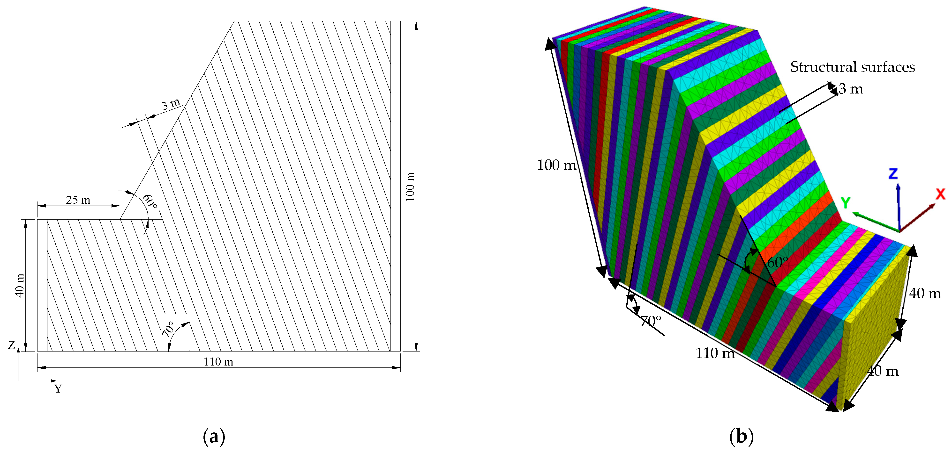
2.1. Overview of the Model

Considering the complexity of three-dimensional dynamic analysis and referring to the relevant results of dynamic analysis carried out by two-dimensional and three-dimensional numerical simulation, the adopted numerical model is shown in Figure 1. The slope angle α = 60° and the dip angle of rock layer β = 70°. The length*width*height of the model is 110*40*100 m, the slope height is 60 m, and the structural surfaces are equidistantly distributed with a spacing of 3 m.

In the process of dynamic analysis, for rock masses under seismic action, the reduction of their strength, especially tensile strength, usually occurs after the onset of plastic yielding [20]. To simulate this property of rock, the rock mass is subjected to the strain-softening plasticity model, while the structural face is subjected to the Coulomb slip failure model, whose relevant physical and mechanical parameters are shown in

Table 1. Physical and mechanical parameters of rock mass and structural surfaces.

Parameters	Values
Density/kg/m3	2650
Young’s modulus/GPa	10.5
Poisson’s ratio	0.25
Rock cohesion/MPa	1.5
Internal friction angle of the rock/°	45
Rock tensile strength/MPa	0.5
Cohesion of structural surface/MPa	0
Friction angle of structural surface/°	30
Tensile strength of structural surface/MPa	0
Normal stiffness of structural surface/GPa/m	58.33
Tangential stiffness of structural surface/GPa/m	19.44

. The normal stiffness K_n and tangential stiffness K_s of the structural face are obtained by Equations (1) and (2) as follows:

$$K_n=10\max [(K+4G/3)/\mathsf{\Delta }{Z}_{\min }]$$

(1)

$$K_s=K_n(G/E)$$

(2)

where K is the bulk modulus, G is the shear modulus, E is the Young’s modulus, and ΔZ_min is the minimum width in the direction of normal contact of adjacent units in the discrete element model [23].

2.2. Dynamic Setting

Unlike the general static conditions, the numerical analysis under dynamic conditions requires consideration and appropriate setting of the relevant dynamic parameters and conditions. Usually, the model must be run under static (gravity) conditions and must reach the static equilibrium before the dynamic analysis is performed. The grid size of the model is set to 3 m, as Equation (3) must be satisfied to ensure the accurate propagation of stress waves within the rock mass [24]:

$$\mathsf{\Delta }l\le (1/10~1/8)\gamma$$

(3)

where γ is the seismic wave wavelength. The form of damping for the dynamic analysis is Rayleigh damping [25]; see Equation (4):

$$[C]=\alpha [M]+\beta [K]$$

(4)

where [M] is the mass matrix, [K] is the stiffness matrix, and α and β are determined from the critical damping ratio ξ_min and the circular frequency ω_min, according to Equation (5):

$$\alpha ={\xi }_{\min }{\omega }_{\min },\beta ={\xi }_{\min }/{\omega }_{\min }$$

(5)

The dynamic analysis used in this paper is ξ_min = 0.02 and ω_min = 5 Hz. The bottom of the model is set as a viscous (non-reflection) boundary, i.e., independent dampers are set at the bottom of the model in the normal and tangential directions, to provide viscous normal and tangential traction, respectively; the free-field boundary is used on all four sides of the model to simulate the free-field motion present but missing within the structure (Figure 2).

Since the bottom of the model is set as a viscous boundary, the dynamic load must be converted from the acceleration-time history to the velocity-time history, and then to the stress-time history applied to the bottom of the model according to Equations (6) and (7):

$${\sigma }_n=2(\rho C_p)v_n$$

(6)

$${\sigma }_s=2(\rho C_s)v_s$$

(7)

where σ_n and σ_s are the applied normal and tangential shear stresses, ρ is the rock density, C_p and C_s are the longitudinal and transverse wave velocities, and v_n and v_s are the applied normal and tangential velocities.

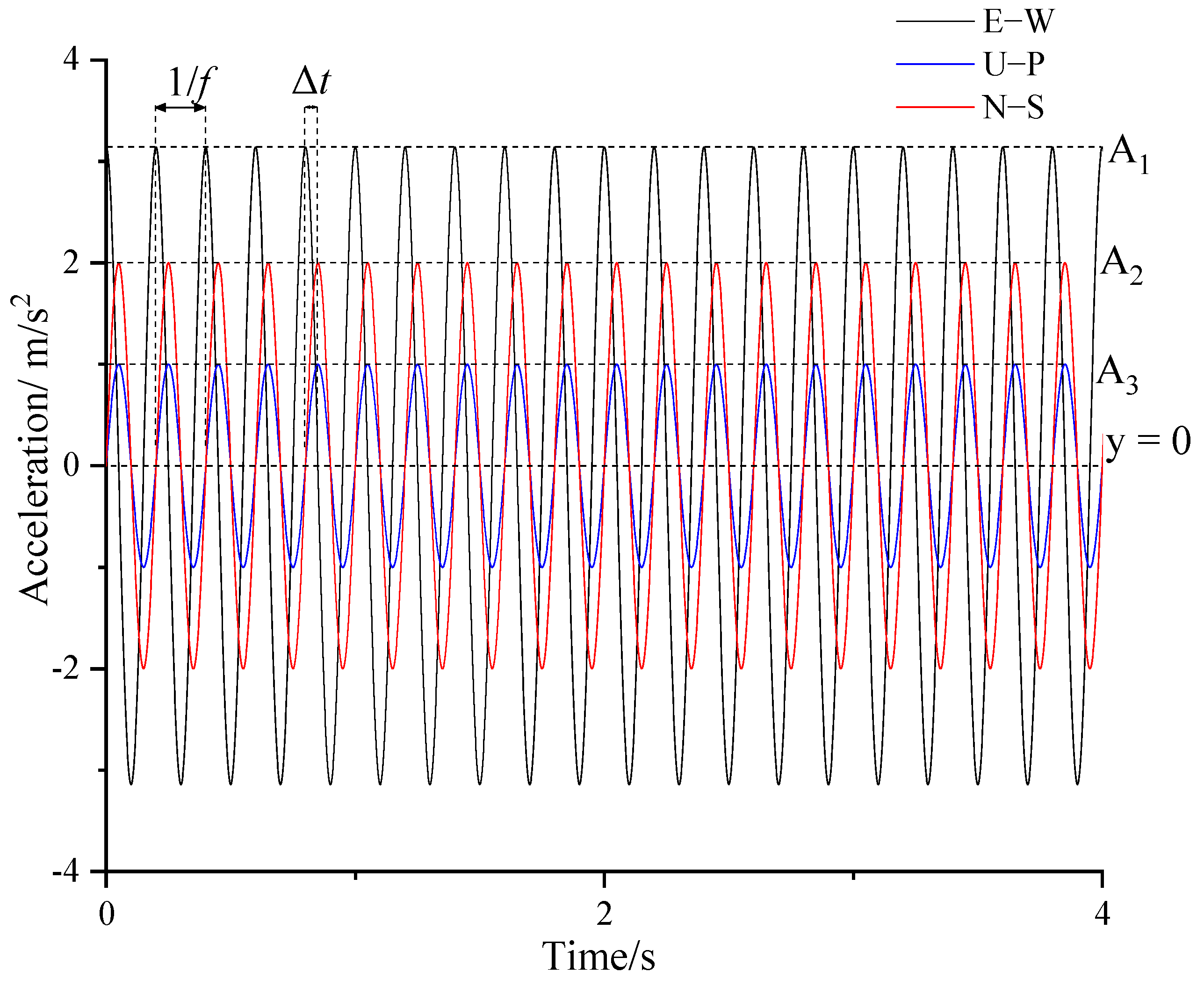
2.3. Loading Conditions

To more intuitively reflect the influence of the variation of each seismic wave parameter, the seismic wave in the form of a sinusoidal wave is selected for loading in this paper (Figure 3). The expression form of the sinusoidal wave three-way acceleration-time history is shown in Equation (8), and the corresponding velocity-time history is shown in Equation (9):

$$a_t=A_n\sin (2\pi ft)$$

(8)

$$v_t=-A_n\cos (2\pi ft)/2\pi f$$

(9)

where n = 1, 2, 3, A₁, A₂ and A₃ correspond to the amplitudes of E−W, U−P and N−S waves, respectively; f is the seismic wave frequency; T is the seismic wave holding time (T = 4 s in the figure); and Δt is the time difference between the peak of the P-wave and the peak of the S-wave.

To truly and objectively reflect the influence of the dynamic parameters of natural seismic waves on the dynamic response and stability of anti-dip slopes under seismic action, the relevant parameters of three natural measured seismic waves are calculated and analyzed, which are shown in

Table 2. Related parameters of natural seismic waves.

Seismic Wave	Seismic Wave Parameters
	Amplitude in U-P Direction (P-Wave) A2/g	S-wave’s Amplitude As/g	Amplitude in E-W Direction A1/g	Amplitude in N-Direction A3/g	Main Frequency f/Hz	Holding Time T/s	Time Difference between P-Wave’s Peak and S-Wave’ Peak Δt/s
Wenchuan Wolong	0.97	1.06	0.98	0.67	1–10	180	21.51
Wenchuan Qingping	0.12	0.11	0.1	0.09	1–10	25	3.54
El Centro	0.21	0.35	0.21	0.34	0.5–15	54	1.14

. For the convenience of analysis, the relationship between the amplitude of the P-wave and the S-wave for the numerical simulation used in this analysis is shown in Equation (10), and the relationship between the amplitude of the S-wave and A₁ and A₃ is shown in Equation (11).

$$A_s=1.1A_2$$

(10)

$$A_s=\sqrt{A_1^2+A_3^2}$$

(11)

To comprehensively analyze the effects of seismic waves, five representative seismic wave parameters are selected for analysis in this paper: S-wave’s amplitude As, S-wave’s incidence direction γ, frequency f, holding time T, and time difference Δt between P-wave’s peak and S-wave’ peak. These are analyzed where γ is defined as the angle between the S-wave’s vector and the slope trend, and the geometric relationship is shown in Equation (12) (Figure 4):

$$\gamma =\arctan (A_3/A_1)$$

(12)

Since these five parameters of seismic waves are independent of each other, to analyze the effects of the parameters in a comprehensive manner, univariate analysis and orthogonal test analysis are used in this paper.

2.3.1. Univariate Analysis

Univariate analysis is used to keep other factors constant, change a variable, and analyze the effect. With reference to the parameters of natural seismic waves in Table 2 and considering the complexity of dynamic analysis, the time range of seismic waves is compressed to a certain extent, and a certain range of values is selected for each parameter, then univariate analysis is performed for each parameter separately. The total 22 loading conditions are shown in

Table 3. Loading conditions of the univariate analysis.

Loading Conditions	Seismic Wave Parameters
	As/g	γ/°	f/Hz	T/s	Δt/s
1	0.2	0	10	3	0.015
2	0.4	0	10	3	0.015
3	0.6	0	10	3	0.015
4	0.8	0	10	3	0.015
5	1.0	0	10	3	0.015
6	0.8	18	10	3	0.015
7	0.8	36	10	3	0.015
8	0.8	54	10	3	0.015
9	0.8	72	10	3	0.015
10	0.8	90	10	3	0.015
11	0.8	0	6	3	0.015
12	0.8	0	8	3	0.015
13	0.8	0	12	3	0.015
14	0.8	0	14	3	0.015
15	0.8	0	10	1	0.015
16	0.8	0	10	2	0.015
17	0.8	0	10	4	0.015
18	0.8	0	10	5	0.015
19	0.8	0	10	3	0.005
20	0.8	0	10	3	0.01
21	0.8	0	10	3	0.02
22	0.8	0	10	3	0.025

.

2.3.2. Orthogonal Test Analysis

The univariate analysis can only analyze the effect of changes in one factor, so the results obtained are relatively one-sided and localized. If the effects of the above five variables are considered simultaneously, assuming four levels of each variable, 4⁵ = 1024 times are required to carry out a full-scale test. To solve this problem, the orthogonal test design method is used in the previous studies on the multi-parameter study of slope stability and even on the dynamic-related problems under seismic action, and good results were achieved [26,27,28,29]. To reduce the workload and to perform the sensitivity analysis of these five parameters of seismic waves, the orthogonal test is adopted. The range of parameter values and factor levels selected for the orthogonal test analysis are shown in

Table 4. Levels of sensitivity analysis of seismic wave parameters.

Level	Seismic Wave Parameters
	As/g	γ/°	f/Hz	T/s	Δt/s
1	0.2	0	6	1	0.005
2	0.4	30	8	2	0.01
3	0.6	60	10	3	0.015
4	0.8	90	12	4	0.02

. The minimum number of trials for the orthogonal test with five factors and four levels is 16, noted as L₁₆(4⁵), and the corresponding loading conditions are shown in

Table 5. Loading conditions of the orthogonal test analysis.

Loading Conditions	Seismic Wave Parameters
	As/g	γ/°	f/Hz	T/s	Δt/s
1	0.2	0	6	1	0.005
2	0.2	30	8	2	0.01
3	0.2	60	10	3	0.015
4	0.2	90	12	4	0.02
5	0.4	0	8	3	0.02
6	0.4	30	6	4	0.015
7	0.4	60	12	1	0.01
8	0.4	90	10	2	0.005
9	0.6	0	10	4	0.01
10	0.6	30	12	3	0.005
11	0.6	60	6	2	0.02
12	0.6	90	8	1	0.015
13	0.8	0	12	2	0.015
14	0.8	30	10	1	0.02
15	0.8	60	8	4	0.005
16	0.8	90	6	3	0.01

.

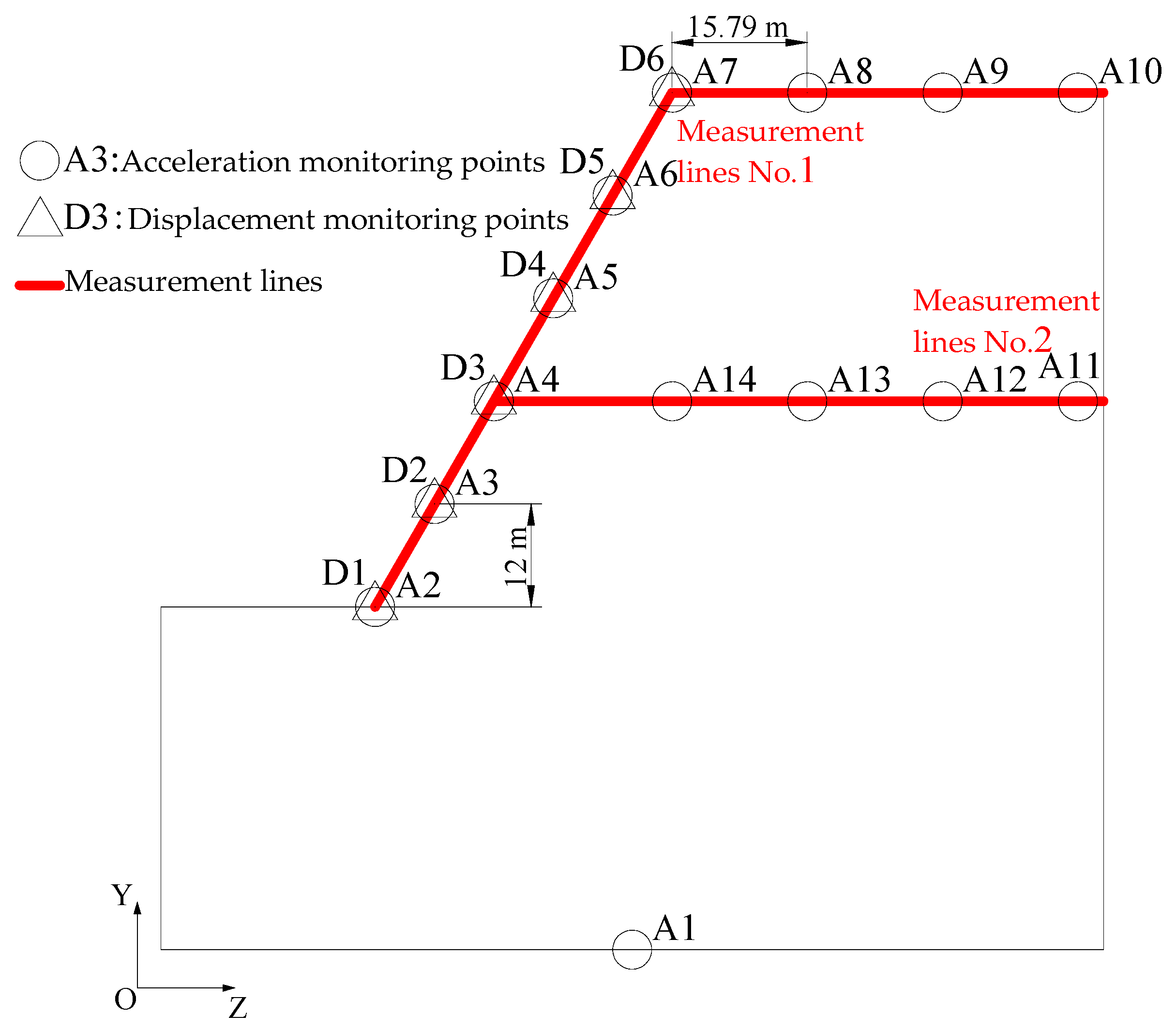
2.4. Arrangement of Monitoring Points

To analyze the effect of seismic wave parameters on the dynamic amplification effect and slope displacement of the slope under seismic action, 15 XYZ three-directional acceleration monitoring points and 6 XYZ three-directional displacement monitoring points are set up on the surface and inside of the slope in the process of dynamic analysis, which are located on two measurement lines to monitor the changes in three-directional acceleration and displacement with time, respectively, in the process of dynamic loading at the corresponding positions of the slope model. The distribution of their corresponding locations is shown in Figure 5. Among them, A1 is located in the center of the bottom of the model, which is used as a reference point to detect the peak acceleration of the seismic wave input to the model. A2-A10 and D1-D6 are equidistantly distributed on the measurement line No. 1, from the slope surface to the top of the slope, which is used to analyze the dynamic response law along the free surface of the slope. A4 and A11–A15 are equidistantly distributed on the measurement line No. 2, and their direction is parallel to the Y axis, from the slope surface of the model slope to the other side, which is used to analyze the dynamic response law inside the slope.

3. Influence of Seismic Wave Parameters on the Dynamic Response of the Slope

The dynamic response of the slope is most intuitively reflected in the increase of acceleration of each part of the slope compared with the initial input dynamic acceleration, i.e., the amplification effect. For the sake of concise and clear analysis, the Peak Ground Acceleration (PGA) amplification factor is used as an indicator to evaluate the amplification effect, i.e., the ratio of the measured PGA to the initial input dynamic PGA at a point inside the slope [18,30,31]. In this paper, the three-dimensional spatial effect is considered, thus the authors write the Acceleration Amplification Factor (AAF) of PGA in X, Y, and Z directions as AAF_x, AAF_y, and AAF_z, and the related expressions are given in Equation (13):

$$\left.\begin{array}{l}AA{F}_x=xPG{A}_n/xPG{A}_0\\ AA{F}_y=yPG{A}_n/yPG{A}_0\\ AA{F}_z=zPG{A}_n/yPG{A}_0\end{array}\right\}$$

(13)

where xPGA_n, yPGA_n, and zPGA_n are the peak accelerations in the X, Y, and Z directions at point n within the model, and xPGA₀, yPGA₀, zPGA₀ are the peak accelerations in the X, Y, and Z directions input at point A1 at the bottom of the model. For slopes, the acceleration in the slope direction, i.e., the Y-direction, is more important for slope stability, so this section analyzes the effect of each seismic wave parameter on the magnitude of AAF_y using the univariate analysis method.

In addition, the stability of slopes is usually determined by the factor of safety F_s under general static conditions. However, under the effect of an earthquake, the magnitude and direction of the external force on the slope change with time, so the dynamic safety factor of the slope is not a constant value. Therefore, with reference to the method of the previous research, the displacement in the slope direction (Y-direction) at the upper part of the slope, i.e., points D4, D5 and D6, are chosen as other indexes for the analysis of the dynamic response of the slope. According to previous studies [17,18], the seismic wave amplitude and holding time are positively correlated with the magnitude of the slope displacement, so this section only focuses on the influence of three parameters such as γ, f, and T on the slope stability by using univariate analysis.

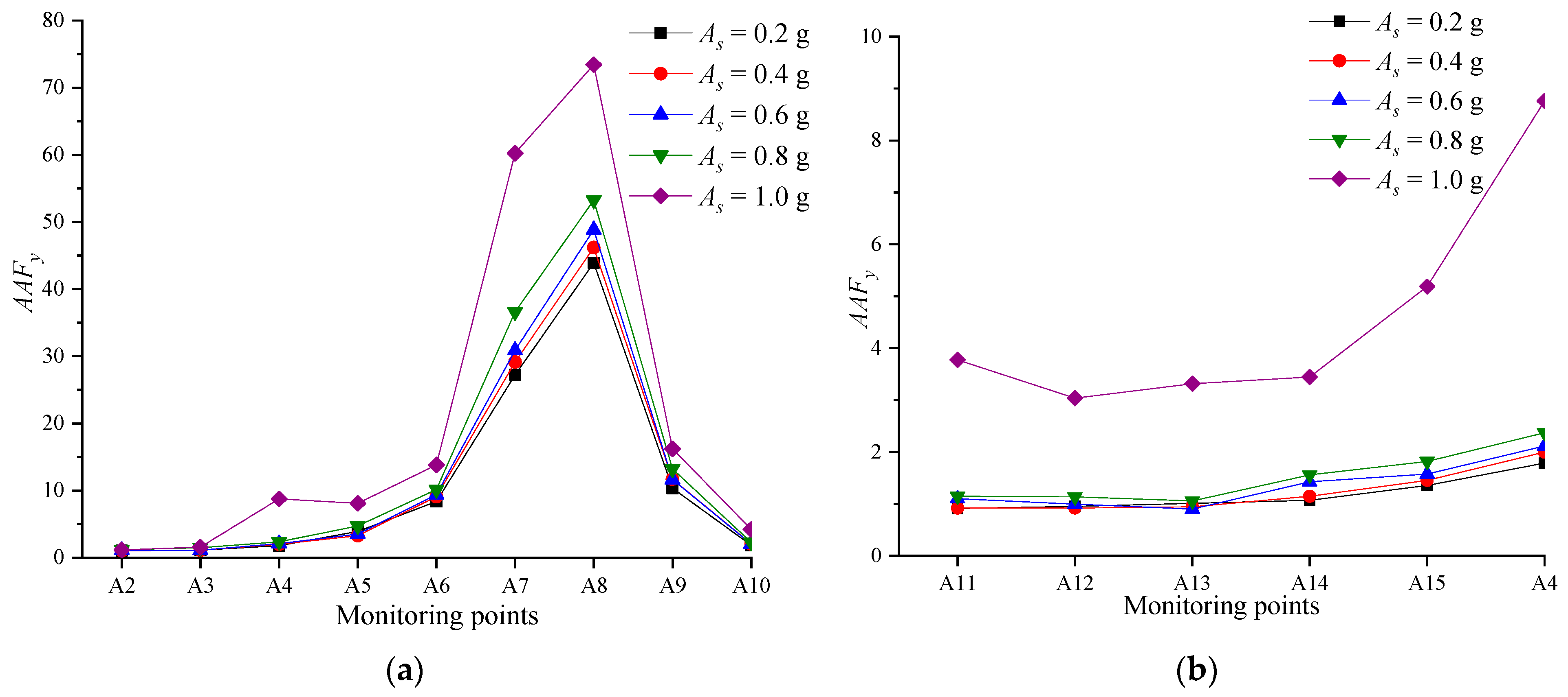
3.1. Effect of S-Wave’s Amplitude A_s

Keeping the remaining four parameters constant, the distribution of the slope amplification coefficient AAF_y under the action of seismic waves with different S-wave amplitudes A_s is shown in Figure 6. The amplification effect of the slope shows an obvious positive correlation with the S-wave’s amplitude A_s. Figure 6a demonstrates that when A_s increases from 0.2 g to 0.8 g, the slope amplification effect of horizontal direction does not increase significantly; however, when A_s increases from 0.8 g to 1.0 g, the amplification effect of the upper part of the slope (three points A7, A8, and A9) increases significantly. This is related to the change of rock structure after the failure of the slope under the strong earthquake: the anti-dip slope has been destabilized by topping, and the bedding rock mass has become fractured, which objectively increases the diffraction of seismic waves in the rock mass and then leads to the exponential increase of the dynamic response.

In addition, according to Figure 6a, the amplification effect of the slope in the lower 3/4 portion is not obvious, but increases significantly in the upper 1/4 portion, which is consistent with the results of the shaking table tests conducted by Huang et al. and Yang et al. The higher dynamic amplification effect of the upper part of the anti-dip slope also causes the upper shoulder part of the slope firstly to fail by ejection and toppling, which has been found in the post-earthquake site of anti-dip slopes in the Wenchuan earthquake and other large earthquakes.

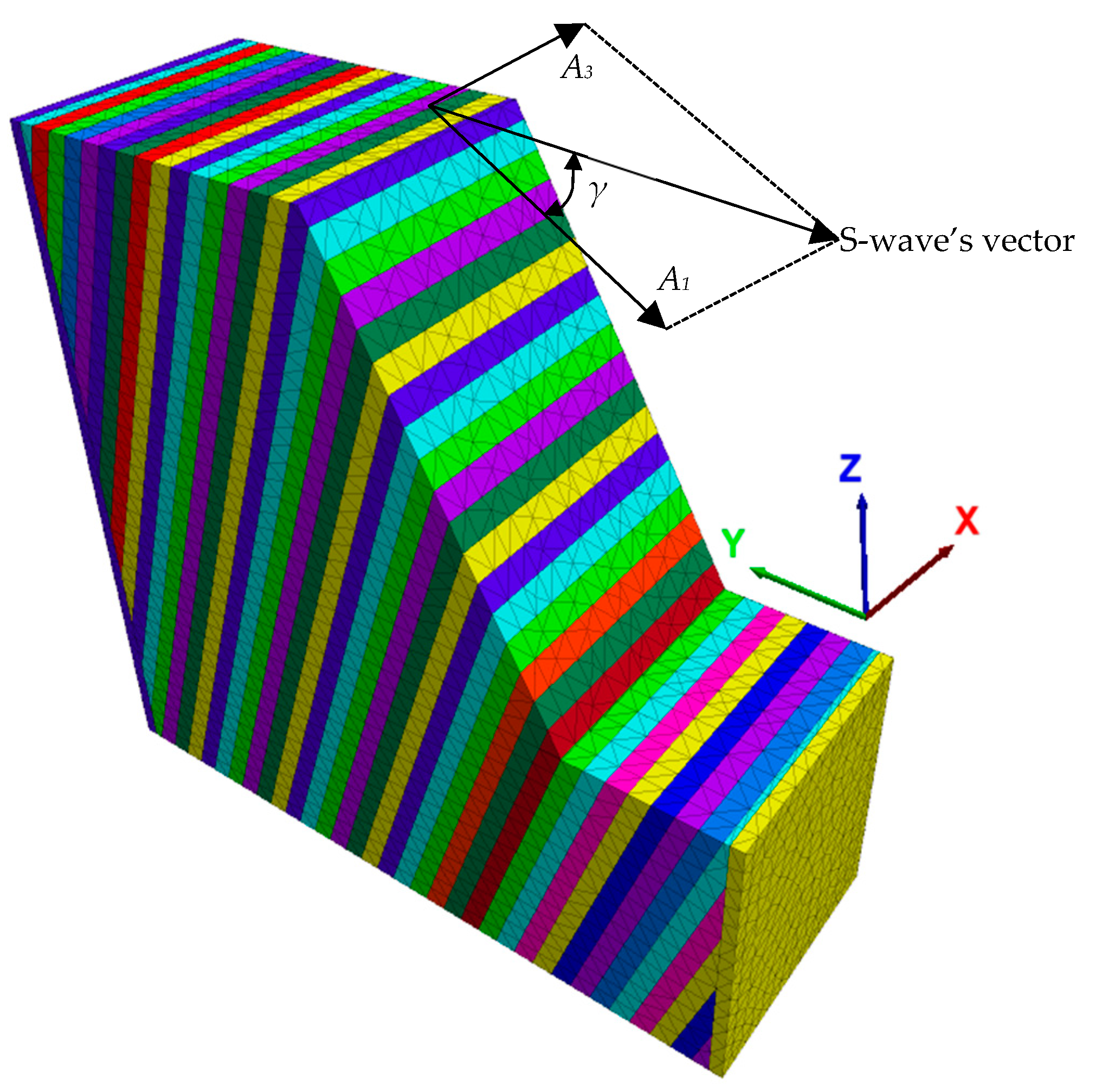
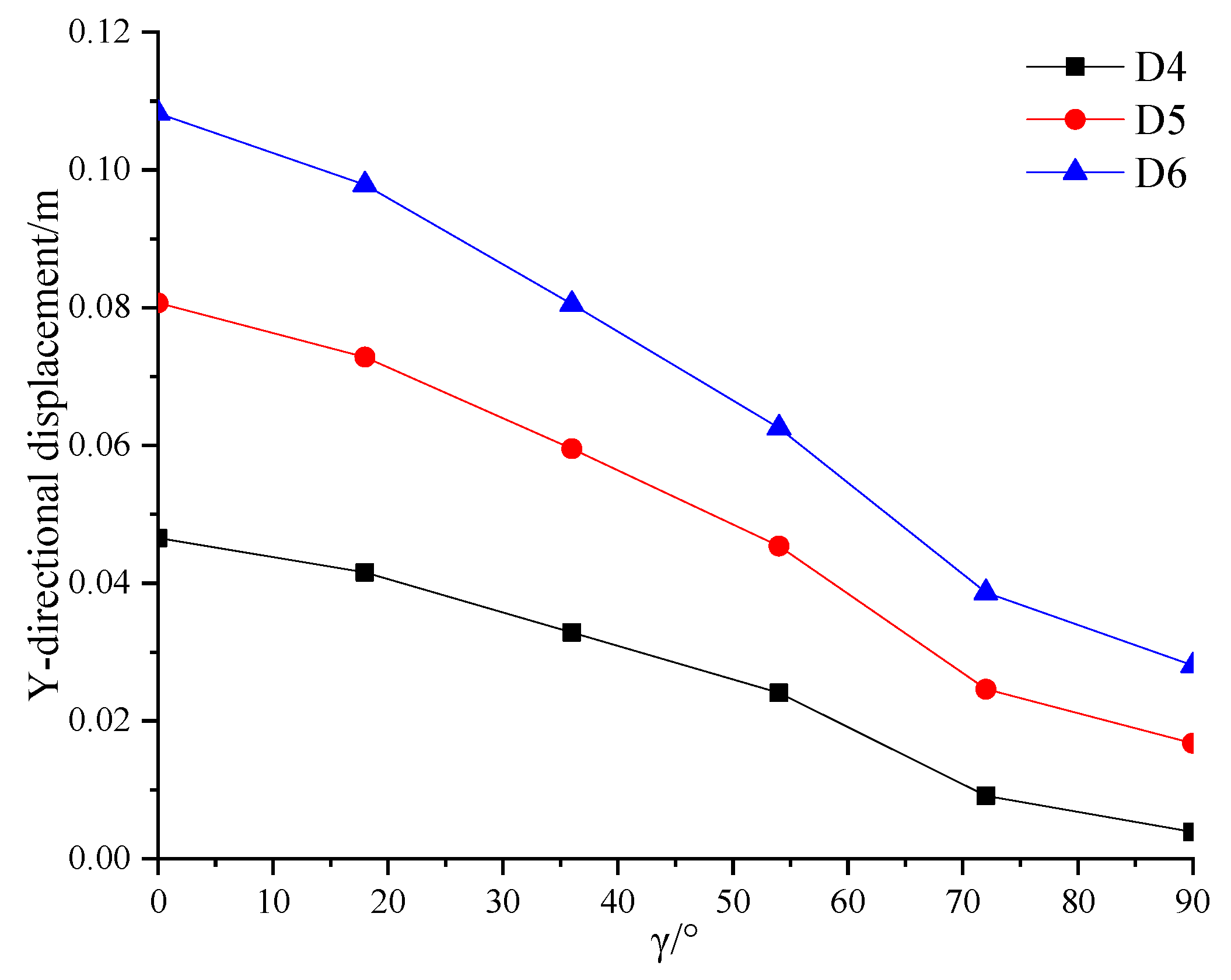
3.2. Effect of the S-Wave’s Incident Direction γ

Keeping the remaining four parameters constant, the distribution of the slope amplification factor AAF_y under the action of seismic waves with different S-wave incidence directions γ is shown in Figure 7. It can be observed from Figure 7a that, with the exception of a few points in the upper part, the variation of AAF_y from bottom to top in the vertical direction of the slope with the value of γ is not significant, and it can be speculated that the amplification law of the slope from bottom to top in the vertical direction, i.e., the “elevation effect,” is only related to the P-wave, while the influence of the incident angle of the S-wave has less influence. Figure 7b shows that the magnitude of AAF_y in the horizontal direction also shows a positive correlation with the value of γ. With the increase of γ to 36°, the law of the horizontal amplification effect of the slope no longer shows a single law of “surface effect,” but shows the rhythm of increasing, then decreasing, and then increasing again. This phenomenon demonstrates that the different incidence angles of the S-wave will directly change the wave propagation law in the rock mass, causing it to be more complicated and irregular, and thus it will no longer show a simple single correlation law.

According to Figure 8, it is obvious that the Y-directional slope displacement is negatively correlated with the value of γ. After γ > 70°, the decrease rate of Y-directional displacement decreases as γ increases. When the incident direction of the S-wave coincides with the slope direction, i.e., γ = 0°, the force generated by the S-wave acts directly on the slope surface, thus the external force on the slope is stronger and the slope stability is lower. As γ increases, part of the seismic force generated by the S-wave is perpendicular to the slope direction, and its influence on the slope stability then decreases.

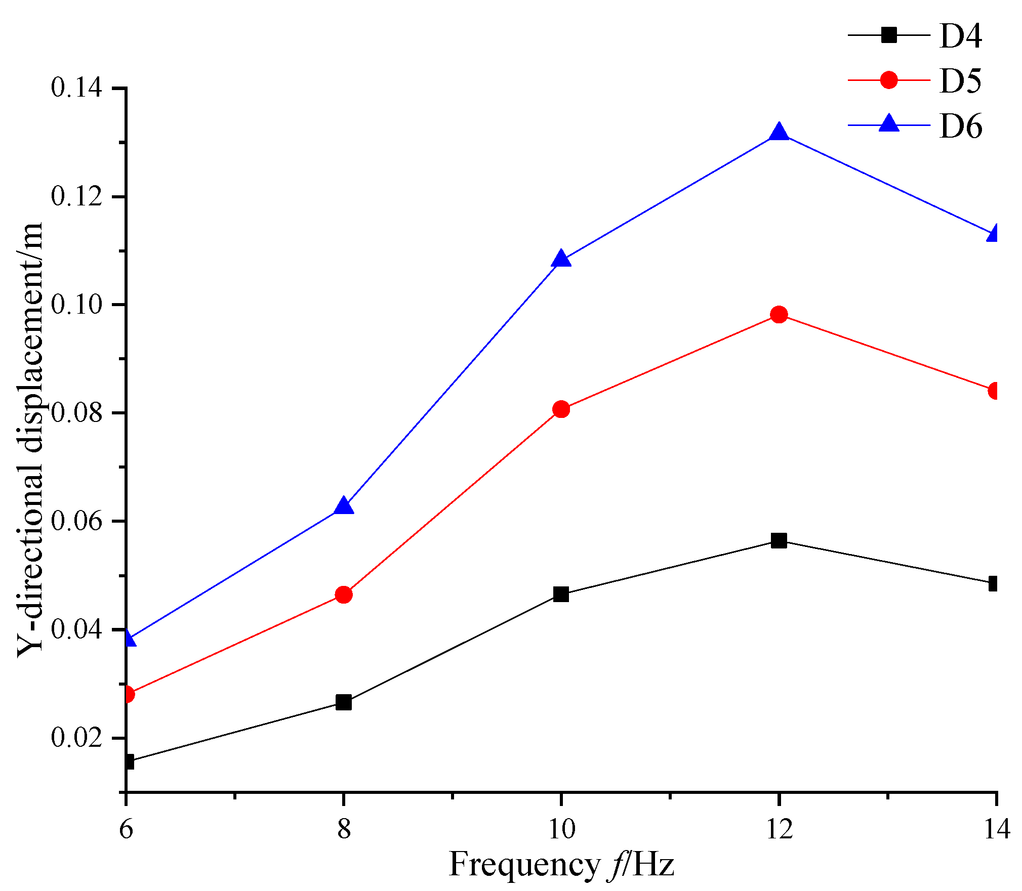
3.3. Effect of Seismic Wave Frequency f

Keeping the remaining four parameters constant, the distribution of the slope amplification factor AAF_y under the action of seismic waves with different frequencies f is shown in Figure 9. As observed in the figure, compared with the results in Section 3.1 and Section 3.2, the frequency f of the seismic wave does not change the law of the amplification effect of the slope along both directions. When f = 12 Hz, the value of AAF_y at each monitoring point is the largest, indicating that the inherent frequency of the anti-dip rock slope model is close to 12 Hz. When the seismic wave frequency is similar to the inherent frequency, the slope will produce the resonance phenomenon, which is then reflected in the stronger dynamic response.

The distribution of Y-directional displacements at points D4, D5, and D6 under different f is shown in Figure 10. The slope-facing displacements increase and then decrease with the increase of seismic wave frequency f, and the extreme value appears at f = 12 Hz. This law coincides with the law of slope dynamic response obtained in Figure 9: at f = 12 Hz, the seismic wave frequency is close to the inherent frequency of the slope, the slope resonates, and the dynamic effect is the strongest. As a result, the displacement is the largest and the slope stability is the worst.

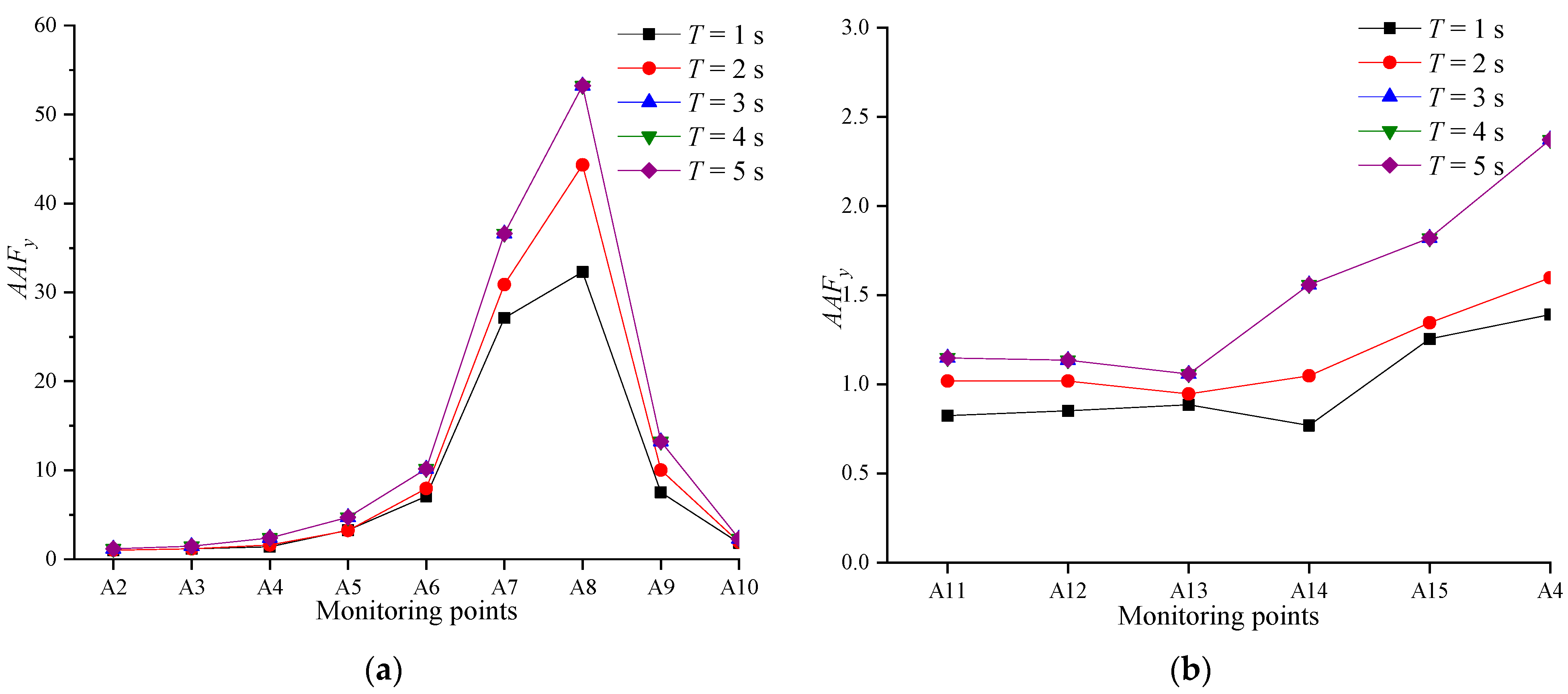
3.4. Effect of Seismic Wave Holding Time T

Keeping the remaining four parameters constant, the distribution of the slope amplification coefficient AAF_y under the action of seismic wave with different holding times T is shown in Figure 11. The analysis results show that when T < 3 s, the amplification effect of the slope increases with the increase of holding time T; when T ≥ 3 s, the value of AAF_y at each point has been kept constant. This indicates that the peak of the amplificati on effect of the slope appears at a certain time point. Thereafter, the slope is destabilized, followed by the generation of the failure surface and the loosening of the rock structure. The propagation of seismic waves within the slope is blocked due to the bending and topping failure of the anti-dip slope, and the structural surfaces open to produce gaps, thus the dynamic response gradually weakens.

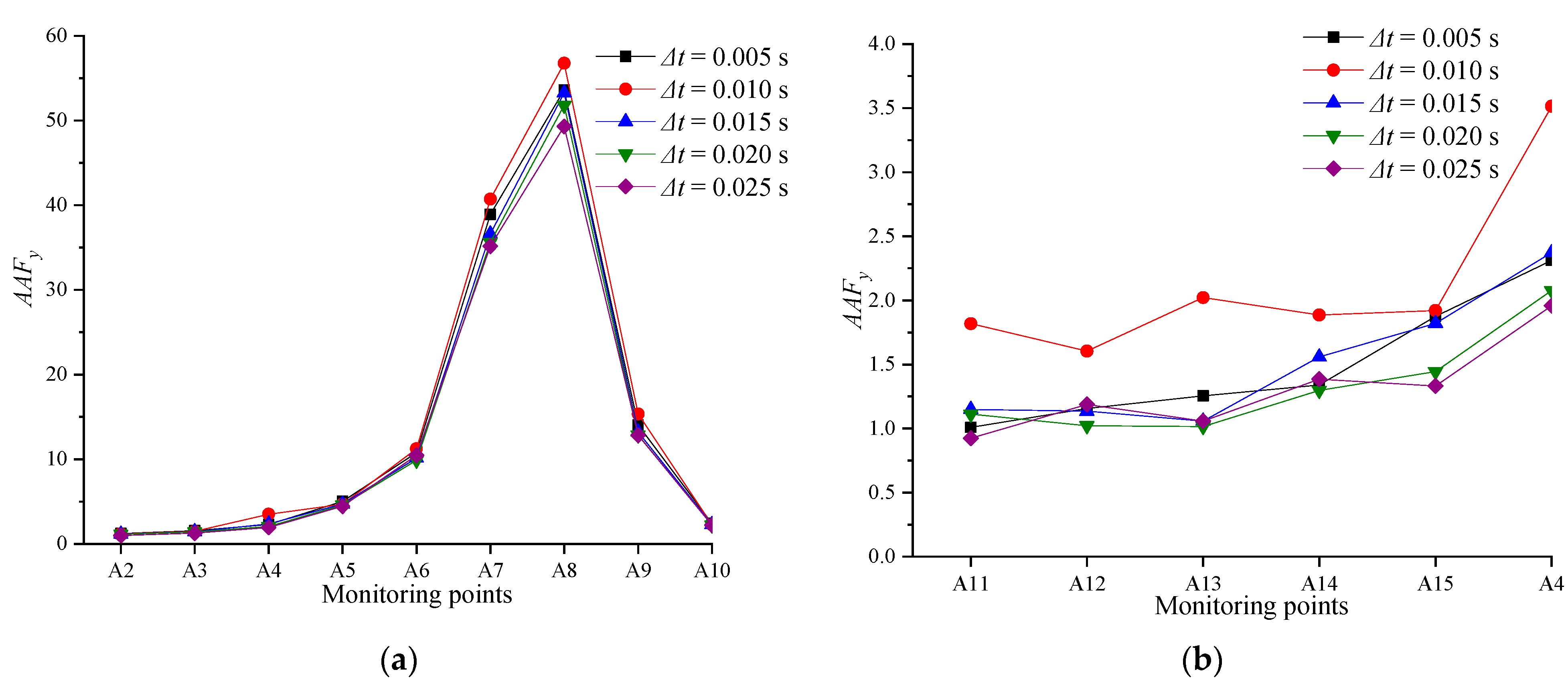
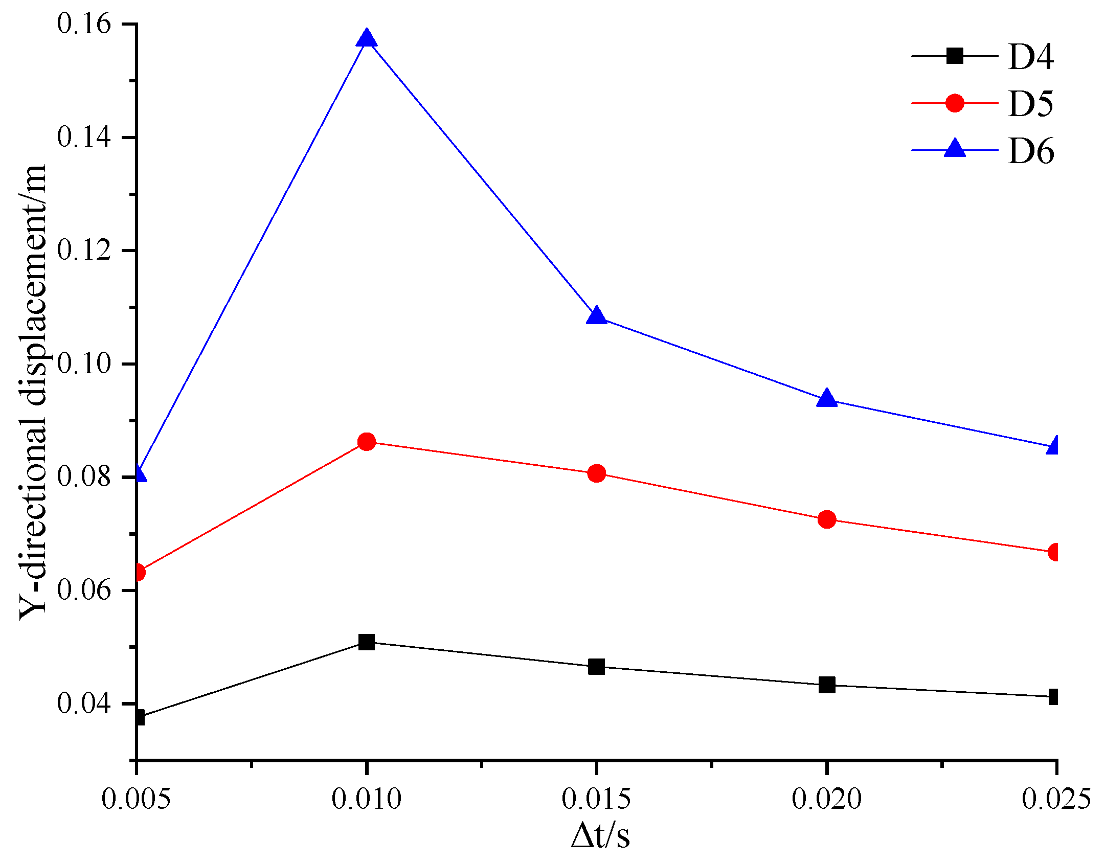
3.5. Effect of Time Difference Δt between the P-Wave’s Peak and the S-Wave’ Peak

Keeping the remaining four parameters constant, the distribution of the slope amplification factor AAF_y under the action of a seismic wave with different time difference Δt between the P-wave’s peak and the S-wave’ peak is shown in Figure 12. Figure 12 demonstrates that the value of AAF_y at each point is the largest when Δt = 0.01 s; when Δt increases from 0.005 s to 0.025 s, AAF_y increases and then decreases. The difference of Δt directly affects the propagation and superposition of the P-wave and the S-wave after incident on the slope, and then leads to the difference in slope dynamic response or amplification effect. Therefore, it can be inferred from the obtained results that when Δt = 0.01 s, the diffraction superposition of seismic waves reaches its peak, and the dynamic response of the slope is the strongest.

The distribution of slope Y-directional displacements at D4, D5, and D6 under different Δt is shown in Figure 13. Similarly, the slope-facing displacements increase and then decrease as Δt increases. This result confirms the rule reflected in Figure 12: when Δt = 0.01 s, the combined superposition effect of the P-wave and the S-wave is the strongest, and the dynamic response of the slope reaches the peak. At this time, the displacement produced by the earthquake is the largest and the slope stability is the worst.

4. Sensitivity Analysis of Seismic Wave Parameters on the Dynamic Responses of Slopes

According to the results in Section 3, it may be concluded that the amplification effect of anti-dip slopes under seismic action has an “elevation effect,” i.e., the acceleration amplification effect of the slope increases with the increase of the slope elevation, thus the acceleration amplification coefficient in the Y direction at points A7 and A8 is the largest. In addition, the common failure mode of anti-dip slopes is bending and topping failure [32,33,34]. Therefore, the Y-directional (slope direction) acceleration amplification coefficient at the shoulder of the slope, which is located at this critical surface of the slope, often plays a decisive role in the stability of anti-dip rock slopes. Thus, the Y-directional acceleration amplification coefficient at the slope shoulder, i.e., point A7, is selected as the analysis index of the orthogonal test, which is denoted as AAF_y7. The results of 16 loading conditions designed for the orthogonal test are shown in

Table 6. Results obtained from the orthogonal test.

Loading Condition No.	Seismic Wave Parameters					AAFy7
	As/g	γ/°	f/Hz	T/s	Δt/s
1	0.2	0	6	1	0.005	36.61
2	0.2	30	8	2	0.010	37.52
3	0.2	60	10	3	0.015	37.70
4	0.2	90	12	4	0.020	37.46
5	0.4	0	8	3	0.020	36.94
6	0.4	30	6	4	0.015	37.87
7	0.4	60	12	1	0.010	38.08
8	0.4	90	10	2	0.005	38.14
9	0.6	0	10	4	0.010	35.72
10	0.6	30	12	3	0.005	37.88
11	0.6	60	6	2	0.020	44.17
12	0.6	90	8	1	0.015	37.16
13	0.8	0	12	2	0.015	35.66
14	0.8	30	10	1	0.020	40.16
15	0.8	60	8	4	0.005	50.50
16	0.8	90	6	3	0.010	60.29

.

4.1. Range Analysis

To objectively assess the sensitivity of these five parameters of seismic waves on the stability of anti-dip rock slopes, the results of the obtained orthogonal tests are analyzed using range analysis. In the orthogonal test, factors A, B...... are selected for the analysis, assuming that each factor has r levels, and the value of the ith level of the j factor is denoted as X_ij, and the test results obtained from each test group are X_k, and X_ij obey normal distribution. Where i = 1, 2…; j = A, B, …, k = 1, 2, …, n., the following relations are formed:

$$K_{ij}={\displaystyle \sum _{k=1}^n{X}_k}$$

(14)

$$k_{ij}=\frac{K_{ij}}{P}$$

(15)

P trials are conducted for each factor at each level, and the extreme difference R_j for factor j is calculated as in Equation (16):

$$R_j=\max \left\{k_{1j},\right.k_{2j}\cdot \cdot \cdot \left.k_{rj}\right\}-\min \left\{k_{1j},\right.k_{2j}\cdot \cdot \cdot \left.k_{rj}\right\}$$

(16)

The larger the extreme difference, the greater the influence of the change in the level of the factor on the test results, and the factor with the largest extreme difference is also the most dominant factor [35,36]. The range analysis is performed based on the results in Table 6, and the obtained results are shown in

Table 7. Results of sensitivity analysis of seismic wave parameters.

Factor	Seismic Wave Parameters
	As	γ	f	T	Δt
K1j	37.32	36.23	44.74	38.00	40.78
K1j	37.75	38.35	40.53	38.87	42.90
K1j	38.73	42.61	37.93	43.20	37.10
K1j	46.65	43.26	37.27	40.39	39.68
Rj	9.33	7.03	7.47	5.20	5.80
Sensitivity	As > f > γ > Δt > T

. For the effect of the strength of the dynamic response of the anti-dip slope, the sensitivity of each seismic wave parameter was ranked as A_s > f > γ > Δt > T. Thus, it can be observed that the S-wave’s amplitude A_s is the decisive factor for the dynamic response of the slope. The higher the seismic intensity, the higher the amplification factor of slope acceleration in the upper part of the slope, especially at the shoulder, which then generates stronger peak acceleration and seismic force, and thus the higher the probability of slope instability. This also confirms the law obtained from the univariate analysis in Section 3.1. On the contrary, the holding time T of the seismic wave has the lowest sensitivity to the dynamic response. The dynamic response of the slope is directly related to the peak response acceleration, which has a strong transient nature, and thus the value of the holding time of the seismic wave has a relatively small effect on the dynamic response of the slope.

4.2. Multiple Regression Analysis of the Acceleration Amplification Effect of the Slope

With the Y-directional acceleration amplification factor AAF_y7 at point A7 as the only dependent variable, and the corresponding five parameters of the seismic wave as independent variables, the model is described as Equation (17):

$$AA{F}_{y7}={\beta }_0+{\beta }_1{A}_s+{\beta }_2\sin \gamma +{\beta }_{3}f+{\beta }_{4}T+{\beta }_5\mathsf{\Delta }t$$

(17)

where β₀, β₁, β₂, β₃, β₄, and β₅ are regression coefficients. Least squares estimation of β₀, β₁, β₂, β₃, β₄, and β₅ in the multiple regression model Equation (16) is done using the least squares method. Let b₀, b₁, b_2, b₃, b₄, and b₅ be the least squares estimates of β₀, β₁, β₂, β₃, β₄, and β₅, respectively, and the following equation is generated:

$$\widehat{AA{F}_{y7}}=b_0+b_1{A}_s+b_2\sin \gamma +b_{3}f+b_{4}T+b_5\mathsf{\Delta }t$$

(18)

where $\widehat{AA{F}_{y7}}$ is a one squares estimate of the minimum of AAF_y7. Perform multiple linear regression on the 16 groups of results in Table 6, and the following regression equation may be obtained:

$$\begin{array}{l}\widehat{AA{F}_{y7}}=39.16526\pm 6.10896+14.4825A_s+\\ 7.37531\sin \gamma -1.24975f+1.1485T+1.1485\mathsf{\Delta }t\end{array}$$

(19)

In the formula, the coefficient of determination R₂ = 0.7295. On the premise of determining the relevant parameters of seismic waves, Equation (19) provides an empirical formula for quantitative evaluation of the dynamic response of anti-dip rock slopes under seismic action. Under the condition that the seismic waves are determined, the peak slope accelerations of anti-dip rock slopes under seismic action can be obtained by combining Equation (13), and then the maximum horizontal seismic force may be determined. This equation provides a theoretical basis for the stability evaluation of anti-dip rock slopes in high seismic intensity areas and for the assessment of landslide hazards.

5. Conclusions

In this paper, the dynamic analysis of the anti-dip rock slope under the action of the sinusoidal seismic wave is carried out by using the three-dimensional discrete element numerical analysis method. Based on the obtained results, the univariate analysis method and the orthogonal test method are used to study the effects of five seismic wave parameters, including seismic wave amplitude, S-wave incident angle, frequency, duration, and P-wave and S-wave peak time differences on the dynamic amplification factor and slope displacement of anti-dip rock slopes, as well as the sensitivity of these parameters to the dynamic response of the slope. The following conclusions were drawn:

• The amplitude A_s and the holding time T of the seismic S-wave are positively correlated with the acceleration amplification effect of the slope, but the acceleration amplification effect of the slope remains unchanged after the latter reaches 3 s. The increase of the S-wave’s incident angle γ changes the distribution law of the acceleration amplification effect along the horizontal direction inside the slope. With the increase of frequency f and the time difference Δt between the peak of the P-wave and the S-wave, the acceleration amplification effect of the slope is first enhanced and then weakened.
• The S-wave’s incident angle γ is negatively correlated with the slope displacement. The increase of frequency f and the time difference Δt between the peak of the P-wave and the S-wave will lead to the first increase and then decrease of the slope Y-directional displacement.
• The sensitivity of each seismic wave parameter is ranked as follows: S-wave’s amplitude A_s > frequency f > S-wave’s incident angle γ > time difference between the P-wave’s and the S-wave’s peak Δt > holding time T. The S-wave’s amplitude A_s of seismic wave is the most critical factor in the slope dynamic response.
• The linear regression equation of the Y-directional acceleration amplification coefficient at the shoulder of the anti-dip rock slope obtained by using multiple regression analysis is $\begin{array}{l}\widehat{AA{F}_{y7}}=39.16526\pm 6.10896+14.4825A_s+\\ 7.37531\sin \gamma -1.24975f+1.1485\mathrm{T}+1.1485\mathsf{\Delta }t\end{array}$. This equation can be adopted to empirically evaluate the magnitude of the dynamic response of the anti-dip rock slope under seismic action, and then provide a theoretical basis for slope stability evaluation.

References

1. Zhang, Z. Principles of Engineering Geological Analysis; Press Geology: Beijing, China, 2009. [Google Scholar]
2. Huang, R. Geodynamic process and stability control of high rock slope development. Chin. J. Rock Mech. Eng. 2008, 27, 1525–1544. [Google Scholar]
3. Xue, Y.; Kong, F.; Yang, W.; Qiu, D.; Su, M.; Fu, K.; Ma, X. Main unfavorable geological conditions and engineering geological problems along Sichuan—Tibet railway. Chin. J. Rock Mech. Eng. 2020, 39, 445–468. [Google Scholar]
4. Huang, F.; Huang, J.; Jiang, S.; Zhou, C. Landslide displacement prediction based on multivariate chaotic model and extreme learning machine. Eng. Geol. 2017, 218, 173–186. [Google Scholar] [CrossRef]
5. Huang, F.; Tao, S.; Chang, Z.; Huang, J.; Fan, X.; Jiang, S.-H.; Li, W. Efficient and automatic extraction of slope units based on multi–scale segmentation method for landslide assessments. Landslides 2021, 18, 3715–3731. [Google Scholar] [CrossRef]
6. Guo, Z.; Shi, Y.; Huang, F.; Fan, X.; Huang, J. Landslide susceptibility zonation method based on C5. 0 decision tree and K–means cluster algorithms to improve the efficiency of risk management. Geosci. Front. 2021, 12, 101249. [Google Scholar] [CrossRef]
7. Huang, F.; Chen, J.; Liu, W.; Huang, J.; Hong, H.; Chen, W. Regional rainfall–induced landslide hazard warning based on landslide susceptibility mapping and a critical rainfall threshold. Geomorphology 2022, 408, 108236. [Google Scholar] [CrossRef]
8. Li, Z.; Hu, Z.; Liu, W.; Hu, G.; Du, S.; Zhou, Y. Plastic limit analysis of open–pit mine jointed rock slope considering translation–rotation mechanisms. Chin. J. Rock Mech. Eng. 2018, 37, 4056–4068. [Google Scholar]
9. Xiao, S.; Liu, H.; Yu, X. Analysis method of seismic overall stability of soil slopes retained by gravity walls anchored horizontally with flexible reinforcements. Rock Soil Mech. 2020, 41, 1836–1844. [Google Scholar]
10. He, J. Research on Structural Effects of Ground Vibration Response Law of Slope. Ph.D. Thesis, Institute of Geology and Geophysics, Chinese Academy of Sciences, Beijing, China, 2020. [Google Scholar]
11. Yang, C.; Zhang, J.; Zhou, D. Research on time–frequency analysis method for seismic stability of rock slope subjected to SV wave. Chin. J. Rock Mech. Eng. 2013, 32, 483–491. [Google Scholar]
12. Newmark, N.M. Effects of earthquakes on dams and embankments. Geotechnique 1965, 15, 139–160. [Google Scholar] [CrossRef]
13. Jibson, R.W. Predicting earthquake–induced landslide displacements using Newmark’s sliding block analysis. Transp. Res. Rec. 1993, 1411, 9–17. [Google Scholar]
14. Romeo, R. Seismically induced landslide displacements: A predictive model. Eng. Geol. 2000, 58, 337–351. [Google Scholar] [CrossRef]
15. Qin, Y.; Tang, H.; Deng, Q.; Yin, X.; Dan, L. Improvement on the calculation method of slope critical acceleration under strong earthquake. Chin. J. Rock Mech. Eng. 2019, 38, 3439–3447. [Google Scholar]
16. Huang, R.; Li, G.; Ju, N. Shaking table test on strong earthquake response of stratified rock slopes. Chin. J. Rock Mech. Eng. 2013, 32, 865–875. [Google Scholar]
17. Yang, G.; Ye, H.; Wu, F.; Qi, S.; Dong, J. Shaking table model test on dynamic response characteristics and failure mechanism of antidip layered rock slope. Chin. J. Rock Mech. Eng. 2012, 31, 2214–2221. [Google Scholar]
18. Yang, G.; Qi, S.; Wu, F.; Zhan, Z. Seismic amplification of the anti–dip rock slope and deformation characteristics: A large–scale shaking table test. Soil Dyn. Earthq. Eng. 2018, 115, 907–916. [Google Scholar] [CrossRef]
19. Zhang, Z.; Wang, T.; Wu, S.; Tang, H. Rock toppling failure mode influenced by local response to earthquakes. Bull. Eng. Geol. Environ. 2015, 75, 1361–1375. [Google Scholar] [CrossRef]
20. Zheng, Y.; Wang, R.; Chen, C.; Sun, C.; Ren, Z.; Zhang, W. Dynamic analysis of anti–dip bedding rock slopes reinforced by pre–stressed cables using discrete element method. Eng. Anal. Bound. Elem. 2021, 130, 79–93. [Google Scholar] [CrossRef]
21. Wu, D. Seismic Safety Evaluation Methods of Layered Rock Slopes Based on the Critical Displacement. Ph.D. Thesis, Institute of Rock and Soil Mechanics, Chinese Academy of Sciences, Wuhan, China, 2021. [Google Scholar]
22. Zhang, K. Study on Dynamic Response of Layered Rock Slope Induced by Earthquake through Numerical Simulation. Master’s Thesis, China University of Geosciences (Beijing), Beijing, China, 2020. [Google Scholar]
23. Itasca. 3DEC–3 Dimensional Distinct Element Code (Version 5.2); Itasca Consulting Group: Minneapolis, MN, USA, 2019. [Google Scholar]
24. Kuhlemeyer, R.L.; Lysmer, J. Finite element method accuracy for wave propagation problems. J. Soil Mech. Found. Div. 1973, 99, 421–427. [Google Scholar] [CrossRef]
25. Shi, C.; Chu, W.; Zheng, W. Technology of Block Discrete Element Numerical Simulation and Engineering Application; China Construction Industry Press: Beijing, China, 2016. [Google Scholar]
26. Zhang, X.; Gong, X.; Xu, R. Orthogonality analysis method of sensibility on factor of slope stability. China J. Highw. Transp. 2003, 16, 36–39. [Google Scholar]
27. Wen, C. Study of yield acceleration of slope stabilized by multistage retaining earth structures and sensitivity analysis of influence factors. Rock Soil Mech. 2013, 34, 2889–2897. [Google Scholar]
28. Li, J.; Su, Y.; Sun, Z.; Zhao, C. 3D seismic displacement analysis method of stepped slopes reinforced with piles based on Newmark principle. Rock Soil Mech. 2020, 41, 2785–2795. [Google Scholar]
29. Fu, H.; Liu, J.; Zhang, L. Dynamic stability analysis for rock slope based on orthogonal test. J. Cent. South Univ. (Sci. Technol.) 2011, 42, 2853–2859. [Google Scholar]
30. Rizzitano, S.; Cascone, E.; Biondi, G. Coupling of topographic and stratigraphic effects on seismic response of slopes through 2D linear and equivalent linear analyses. Soil Dyn. Earthq. Eng. 2014, 67, 66–84. [Google Scholar] [CrossRef]
31. Song, D.; Che, A.; Zhu, R.; Ge, X. Dynamic response characteristics of a rock slope with discontinuous joints under the combined action of earthquakes and rapid water drawdown. Landslides 2018, 15, 1109–1125. [Google Scholar] [CrossRef]
32. Goodman, R.E. Toppling of rock slopes. In Proceedings of the Speciality Conference on Rock Engineering for Foundation and Slopes, Boulder, CO, USA, 15–18 August 1976; pp. 201–234. [Google Scholar]
33. Adhikary, D.P.; Dyskin, A.V.; Jewell, R.J.; Stewart, D.P. A study of the mechanism of flexural toppling failure of rock slopes. Rock Mech. Rock Eng. 1997, 30, 75–93. [Google Scholar] [CrossRef]
34. Zheng, Y.; Chen, C.; Liu, T.; Zhang, H.; Sun, C. Theoretical and numerical study on the block–flexure toppling failure of rock slopes. Eng. Geol. 2019, 263, 105309. [Google Scholar] [CrossRef]
35. Fang, K.; Ma, C. Orthogonal and Homogeneous Design; Science Press: Beijing, China, 2001. [Google Scholar]
36. Chen, X. Statistics Introduction; Science Press: Beijing, China, 1997. [Google Scholar]
Figure 1. Three-dimensional discrete element model of the slope: (a) side view; (b) three-dimensional spatial view.
Sustainability 14 11321 g001
Figure 2. A schematic diagram of model dynamic boundary conditions: (a) side view; (b) three-dimensional spatial view.
Sustainability 14 11321 g002
Figure 3. Input acceleration-time history in the form of sinusoidal wave for dynamic analysis.
Sustainability 14 11321 g003
Figure 4. The relationship between the angle γ and the spatial position of the slope model.
Sustainability 14 11321 g004
Figure 5. Distribution of acceleration monitoring points, displacement monitoring points, and measurement lines on the slope model.
Sustainability 14 11321 g005
Figure 6. Distribution of acceleration amplification factor AAFy of the slope under different As: (a) measurement line No.1; (b) measurement line No.2.
Sustainability 14 11321 g006
Figure 7. Distributions of acceleration amplification factor AAFy of the slope under different γ: (a) measurement line No.1; (b) measurement line No.2.
Sustainability 14 11321 g007
Figure 8. Distribution of Y-directional displacement of the slope surface under different γ.
Sustainability 14 11321 g008
Figure 9. Distribution of acceleration amplification factor AAFy of the slope under different f: (a) measurement line No.1; (b) measurement line No.2.
Sustainability 14 11321 g009
Figure 10. Distribution of Y-directional displacement of the slope surface under different f.
Sustainability 14 11321 g010
Figure 11. Distribution of acceleration amplification factor AAFy of the slope under different Δt: (a) measurement line No.1; (b) measurement line No.2.
Sustainability 14 11321 g011
Figure 12. Distribution of acceleration amplification factor AAFy of the slope under different Δt: (a) measurement line No.1; (b) measurement line No.2.
Sustainability 14 11321 g012
Figure 13. Distribution of Y-directional displacement of the slope surface under different Δt.
Sustainability 14 11321 g013