Less Water, Less Oil: Policy Response for the Kenyan Future, a CGE Analysis

Abstract

The continuous depletion of nonrenewable natural resources and climate change may lead to a future characterized by a higher frequency of extreme natural events (i.e., flooding, hurricanes, and droughts) and resource supply shocks (i.e., oil price shock). Sub-Saharan African countries will be particularly exposed to these types of shock due to their socioeconomic conditions and geographical conformation. This study investigates the impact of two contemporaneous covariant sudden shocks (i.e., drought and price oil shock) and the possible coping strategies through a static computable general equilibrium (CGE) model for Kenya. The results suggest that a mitigation policy as public transfers is an effective mitigation tool for drought effects, improving welfare and GDP in the short run. However, adopting public transfers during an oil crisis may have regressive effects on population income and welfare. Because the mitigation effectiveness is strongly affected by the complex interaction of combined shocks, the public authorities should pay attention to policy implementation. These findings call for a new scheme of transfer allocation where rural and low-income household quantiles should receive more attention by postdrought mitigation policy, being that they are more vulnerable to external shocks.

1. Introduction

Developing countries, particularly sub-Saharan African countries, have been exposed to various risks and economic shocks over the past century [1]. These events can be wars, financial crises, or extreme weather conditions due to climate change [2]. When the shocks impact the broader population scale (from significant communities of people to the whole country’s population) or register a wider socioeconomic impact, these shocks can be defined as covariate shocks [3]. Covariate risks concern communities, whereas idiosyncratic risks affect one or few households [2]. Idiosyncratic risks are more pronounced among the poor, rural areas due to their dependencies to the agriculture product and their sensitivity to the food price inflation alongside their higher populated household units [4]. Coping strategies for sudden covariate shocks in poor or semipoor African countries have proven to be vital in terms of welfare because of the negative impact of the shock on welfare and the economy. Since most of the population in sub-Saharan African countries lives in rural areas with low-income families, any shock could have a disastrous impact on welfare. For instance, climate change shocks, such as droughts or floods, negatively affect agricultural productivity. Reduction in agricultural productivity, particularly rain-fed production, negatively impacts most African countries that depend heavily on these agricultural products. Moreover, economic shocks (e.g., strong price oscillations) can reduce the ability of rural communities to assess food security and sustainable livelihood by self-consumption or accessing the market commodities [5].

Although the Kenyan economy is one of the largest in the sub-Saharan region, 62.5% of the population lives in rural areas, and 36.8% of the population in 2014 was below the poverty line. (According to the World Bank, the poverty line is defined as a level of income lower than USD 1.9 per day.) Apart from the demographic situation, in recent years, Kenya’s vulnerability has been affected by climate and economic covariate shocks. For example, due to the geographical layout (more than 80% of the available land in Kenya is categorized as arid or semarid land [6]), between 1991 and 2000, Kenya recorded five droughts that affected almost 40 million people due to harsh weather conditions, crop failure, overexploitation of land, and loss of livestock [7]. During one of the most recent droughts (2008/9), it was estimated that 3.5 million people needed immediate food supply, and 6.2 million people were at the starvation level [8]. According to Kenya’s Post-Disaster Needs Assessment [9], the economic damage of the 2010/2011 drought was USD 12.1 billion, and the recovery budget should be around USD 1.7 billion. At the time, the Kenyan government requested a transfer of USD 1.2 billion. Hence, droughts are one of the (climate) events that cause agriculture loss, and crop failure imposes a massive economic impact on the Kenyan economy.

In addition to natural disasters, in recent decades, the world economy has been affected by oil price shocks due to political instability [10].

Table 1. Events in the Kenyan oil sector, 1957–2002 [11].

Origin of the Shock	Date	Recorded Oil Price Increase
Suez Crisis	August 1957	January 1957–February 1957 (9%)
OAPEC embargo (Arab–Israel War)	October 1973	November 1973–February 1974 (51%)
Iranian Revolution	January 1980	May 1979–January 1980 (57%)
Iran–Iraq War controls lifted	July 1981	November 1980–February 1981 (45%)
Gulf War I	July 1990	August 1990–October 1990 (93%)
Venezuela unrest, Gulf War II	December 2002	November 2002–March 2003 (28%)

shows the events that led to the increase in oil prices, consequently impacting the Kenyan oil sector [11].

According to the World Bank [12], oil prices will rise from USD 56 per barrel in 2021 to USD 70 per barrel in 2035. This evolution will become even more relevant to the Kenyan economy. Indeed, according to the Energy and Petroleum Regulatory Authority [13], the rise of domestic oil consumption (+38% and +164% in terms of oil and liquefied petroleum, respectively) led to a growth in oil import of 53% between 2008 and 2018. Despite the significant improvement in oil production since 2012, Kenya is still a net oil-importing country. For net-importing countries, the increase in oil prices leads to higher production costs and a slowdown in the growth rate, reducing domestic output and increasing inflation [14,15].

Unfortunately, two differentiated shocks may happen in the same period. For instance, oil shocks could occur in the period when the country is suffering from famine because of extreme natural events (e.g., in 2014, Kenya faced an oil shock in conjunction with a drought.).

This study addresses the impact of two contemporaneous covariant shocks (i.e., drought and price oil shock) and possible coping strategies through a static computable general equilibrium (CGE) model applied to Kenyan data. The analysis of these shocks and the coping strategies requires a specific social accounting matrix (SAM) describing the linkages between production, income, consumption, and investment of the agents in the economy. This paper employs a modified version of the SAM for Kenya [16], which is aggregated, focusing on the agricultural sector. Hence, for example, all activities not related to agriculture have been aggregated in several macroactivities (e.g., rest of manufacturing or rest of services), whereas those strictly interconnected with it have been maintained separately (e.g., fertilizers (nitrogen) or water).

The analysis implements a static CGE for two main reasons related to the nature of the shocks. First, it allows for examining both the short-run macroeconomic impact of drought on Kenya’s economy and the redistributive consequences of the government’s natural disaster mitigation policy without introducing assumptions about the complex climate dynamics [17,18]. Second, it allows for addressing the short-run effect on a net-importer country of a sudden increase in the oil price, leaving out of the analysis the uncertain evolution of future oil prices.

To the best of the authors’ knowledge, this analysis provides an innovative contribution because the effectiveness of a drought mitigation policy is evaluated during a global oil crisis, whereas the CGE literature addresses it separately (see Section 2). Another aspect that makes this study valuable is the attempt to perform scenario analyses as close as possible to the actual situation in Kenya by adopting a static CGE model. In fact, the scenarios are based on Kenyan past events (droughts) or past international oil crises. We therefore adopted a static CGE model because we explore sudden shocks characterized by abrupt but (relatively) short impacts in a developing country with a high level of vulnerability to poverty and with most of the population living in rural areas. Therefore, mitigation policies should be effective in the short term, and a static CGE is an effective tool to evaluate them.

2. Literature Review

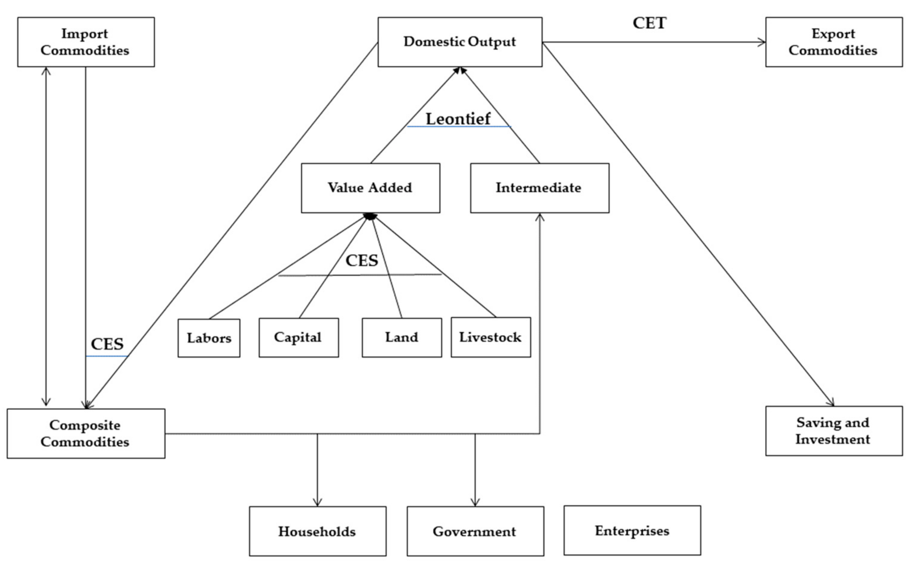
This study ideally bridges two extensive branches of the CGE modeling literature: (i) the one that addresses the impact of external climate shocks (i.e., natural disasters) and (ii) the one that investigates the effect of oil price shocks, extending the analysis on the possible combined effects on welfare and suggesting some policy responses.

By introducing an agriculture production loss scenario, Ref. [19] investigated the impact of drought and food aid policy in Mozambique. This study shows the positive effects of direct food aid on households during drought. Ref. [20] used a similar method to address the impact of drought on the economy of Botswana and to show the effectiveness of different coping strategies (i.e., external food transfers and food vouchers). In the case of Ethiopia (Awash Basin), Ref. [21] quantified the negative impact of drought on GDP as a reduction of 5% with a more substantial effect on the share of GDP produced by agriculture, which decreased by 10%. Ref. [22] showed the impact of drought on Uganda’s economy, highlighting the role of food shortages in economic and welfare losses. In the case of Ethiopia, Ref. [23] showed the negative impact of climate change. Another similar study by [24] on the South African economy showed the unfavorable effects of drought on agriculture. Ref. [8] showed the impacts of extreme weather on Kenya’s growth and economy, whereas [25] found comparable results for the economy of Mozambique.

Looking at the CGE literature that addresses the effect of oil shocks, Ref. [26] investigated the impact of oil shocks on the Kenyan economy, highlighting the adverse effects of oil price jumps on domestic institutions and production. Ref. [27] showed the negative impact of soaring oil prices on the welfare of sub-Saharan countries using static and dynamic CGE models. The author used counterfactual simulations for 2002–2008, showing how Kenya lost 2.1% per year in terms of GDP. From studies on oil shocks in other developing countries, Ref. [28] found that oil shocks may devastate welfare but weakly affect poverty in the short run in India. Ref. [29] performed a comparative study on the impact of an oil price shock coupled with implementing a climate policy in Malaysia.

The empirical literature has deeply investigated the impact of oil prices on developing countries. For instance, using an unrestricted vector autoregressive model, Ref. [30] highlighted the adverse effects of oil prices on net-importing developing countries. In contrast, net-exporting countries are more likely to benefit from it. Comparable findings were shown by [31,32]. Focusing on analyses addressing sub-Saharan African countries, Ref. [33] developed an autoregressive distributed lag model highlighting a considerable impact of oil fluctuations on welfare in the case of Ghana. Ref. [11] performed a comparable analysis of the Kenyan economy, discovering that the main transmission channel of the oil shock to the economy in the short run was consumption.

The rest of the paper is structured as follows: Section 3 describes the methodological approach, Section 4 presents the data and the selected exploration scenarios, Section 5 contains the simulation results, and Section 6 suggests concluding remarks.

3. Methodology

In line with the relevant literature [34,35], we develop a static computable general equilibrium model to address the impact of two sudden shocks within one period (see the supplementary material in Appendix A for the full description of the model).

Figure 1 illustrates the production process. In the production process, domestic producers maximize their profit subject to their production technology (i.e., a constant elasticity of substitution (CES) function. Production technology includes the factor of production, which will be aggregated with intermediate commodities. Intermediate commodities (raw materials) with a fixed share in the Leontief function contribute to the production of one unit of commodities. The composite commodity basket can provide intermediate commodities. In the composite commodity basket, domestic commodities and imported commodities are aggregated with CES technology. The composite commodities price (market price) includes extra taxes, such as sales tax, tariff tax, and, in some cases, additional market margins.

The number of imports is decided according to the Armington assumption. According to this assumption, the composite commodity production equals domestic demand and is the mixture of domestic and imported goods. Domestic demand is the sum of domestic consumption (household units, enterprises, and government) and the domestic producer’s demand (intermediate commodities). Under the baseline assumption, the exchange rate is flexible, and foreign investment (tradeoff between imports and exports in foreign currency) is considered fixed. The savings and investment account is modeled as a fixed share; however, governmental deficit (i.e., savings) is assumed to be flexible to ensure equilibrium in the economy. More details on governmental budget control and market closure can be found in Appendix A.

Households maximize their utility function subject to their budget constraint. Solving the optimization problem, we obtain Equations (1) and (2):

$$P{Q}_{c}Q{H}_{c h}=P{Q}_c{\gamma }_{c h}^m+{\beta }_{c h}^m\left(E{H}_h-{{\displaystyle \sum }}_{c^{\prime }ϵC}P{Q}_{c^{\prime }}{\gamma }_{c^{\prime }h}^m-{{\displaystyle \sum }}_{aϵA}{{\displaystyle \sum }}_{c^{\prime }ϵC}PXA{C}_{a c^{\prime }}{\gamma }_{a c^{\prime }h}^h\right)$$

(1)

$$PXA{C}_{a c}QH{A}_{a c h}=PXA{C}_{a c}{\gamma }_{a c h}^h+{\beta }_{a c h}^h\left(E{H}_h-{{\displaystyle \sum }}_{c^{\prime }ϵC}P{Q}_{c^{\prime }}{\gamma }_{c^{\prime }h}^m-{{\displaystyle \sum }}_{aϵA}{{\displaystyle \sum }}_{c^{\prime }ϵC}PXA{C}_{a c^{\prime }}{\gamma }_{a c^{\prime }h}^h\right)$$

(2)

$$E{H}_h=(1-{{\displaystyle \sum }}_{iϵINSDNG}shi{i}_{i h})\left(1-MP{S}_h\right)\left(1-TIN{S}_h\right)Y{I}_h$$

(3)

According to Equation (1), the total value of the household marketed commodity consumption ($P{Q}_{c}Q{H}_{c h}$) must be equal to the value of the subsistence level of consumption ($P{Q}_c{\gamma }_{c h}^m$) plus the remaining share of income, called supernumerary income. The subsistence level of consumption is the minimum amount needed for each household, whereas extra consumption depends on the household’s income disposal. Gross household income is from factor endowment and transfers from other institutions. Due to the lack of information, we assumed a constant endowment factor. Rental price and wages are endogenous in the baseline version of the model. Equation (3) shows that household net income ($E{H}_h$) is equal to gross income ($Y{I}_h$) minus the direct tax rate paid to the government ($TIN{S}_h$) and the marginal propensity of the saving rate ($MP{S}_h$) paid to the savings and investment account. The household’s gross income is also reduced by transfers to other domestic nongovernmental institutions with the share of $shi{i}_{i h}$. Equation (2) represents the case where households have self-consumption (i.e., households themselves produce goods that they consume). This concept is common to the African economy. The price for these commodities has no tax and margin, which is the difference between the values of consumption in Equation (2) ($PXA{C}_{a c}\times QH{A}_{a c h}$) and Equation (1).

Since we do not have a credit market, the income of each institution should be equal to its expenditure. The subsistence level of consumption should be estimated based on the Fischer parameter [36] for each household type.

$$w_h=-\frac{E{H}_h}{E{H}_h-P{Q}_c{\gamma }_{c h}^m}$$

(4)

The Fischer parameter ($w_h$) is the income elasticity of the marginal utility of income, which can be seen in Equation (4). This parameter is needed to estimate the unknown subsistence level of consumption. To assess the Fischer parameter, we can refer to Equation (5) according to the method developed by [37]:

$$-w\approx 36X^{-3.6}$$

(5)

where w is the Fischer parameter and X is the GNP per capita in US dollar exchanged to Kenyan shilling (KES).

Estimating this parameter is essential for our analysis to get a more accurate picture of the different consumption patterns of varying household quintiles (from rich to poor). As Equation (5) shows, the richer the household, the smaller the Fischer parameter number in absolute value.

From the demand side, the factor market includes domestic and international demanders, and from the supply side, factor owners, such as households and enterprises. Wages can fluctuate according to demand when supply is constant. As with any other market in the CGE model, factor supply must equal factor demand when in equilibrium. Elasticities in this study were derived from estimates made by [38] based on an econometric approach.

4. Data and Simulations

To identify the linkages between drought, agricultural production, food price changes, and welfare losses, we developed a modified version of the 2014 Kenyan social accounting matrix (SAM). The details and specifications of the 195 accounts of the original SAM can be found in [16]. A social account matrix is a comprehensive, economy-wide database reporting the value of all transactions (in this case, expressed in Kenyan shilling) among agents over a period of time, usually 1 year. The new SAM includes 22 activities and 20 marketed goods. The modified SAM takes into account the dual role of households as producers and consumers. This requires separating the production inputs of these households according to their destination: self-consumption and market [39].

Rural household duality and drought are crucial for the agricultural sector. For this reason, the SAM has been aggregated from an agrocentric perspective. SAM classifies agricultural activities into six accounts: coffee, which is the cash crop in Kenya; aggregate food crops; dairy (meat, dairy, and livestock); the rest of agriculture, and two representing households as food- and cash-crop-producing activities.

Households are aggregated into 12 accounts: 5 accounts for each of Kenya’s two major cities (Nairobi and Mombasa), dividing households according to their income in the quintile distribution (from Q1 to Q5), and 2 for the rest of Kenya (rural and urban—without Nairobi and Mombasa). This classification allows us to perform a redistributive analysis of covariate shocks and mitigation policies.

The factors of production are land (irrigated and nonirrigated), capital (agricultural and nonagricultural), livestock, and labor. The labor factor is disaggregated into high-skilled, semiskilled, and unskilled labor, regionalized into four locations (Nairobi, Mombasa, nonirrigated rain-fed areas, and the rest of Kenya).

As a result, the new Kenyan SAM structure has 88 accounts.

Table 2. Modified Kenya SAM 2014.

Accounts	Details	Numbers
Activities	Activities	20
	Household as an activity	2
Commodities	Marketed commodities	20
Factors of production	Labors	12
	Capital	2
	Land	2
	Livestock	1
Domestic nongovernmental institutions	Households	12
	Enterprises	1
Government	Government	1
Taxes	Direct tax	1
	Indirect tax	1
	Factor tax	1
	Sales tax	1
	Tariff on rest of the world	1
Rest of the world	Rest of the world	1
Saving and investment	Investment	1

shows the revised SAM with details and the number of accounts for each group (see Appendix A for further description of activities and accounts).

To capture the economic impact of oil and drought shocks, three main scenarios were designed: scenario A (drought without policy response), scenario B (drought with policy response), and scenario C (drought with policy response and oil shock).

Scenario A is a Hicks-neutral technological shock [22,24]. A shock is defined as Hicks-neutral if it does not change the balance of factors of production in the production function [40]. The Hicks-neutral technological shock will affect the efficiency parameter in the production function, considering a fixed amount of factor supply. We assume that the climate change shock (i.e., drought) reduces the efficiency parameter ${\alpha }_a^{va}$ of Equation (6):

$$QV{A}_a={\alpha }_a^{va}{\left({\displaystyle \sum }_{fϵF}{\delta }_{f a}^{va}Q{F}_{f a}^{-{\rho }_a^{va}}\right)}^{\frac{1}{{\rho }_a^{va}}}$$

(6)

where $QV{A}_a$ is the quantity of value added for activity a, $Q{F}_{f a}$ is the quantity of factor f being demanded in activity a, ${\alpha }_a^{va}$ is the efficiency parameter for activity a, ${\delta }_{f a}^{va}$ is the share of factor f used in activity a, and ${\rho }_a^{va}$ is a value-added function exponent. In line with the reference literature [21,41,42,43], the amount of average reduction across all agriculture commodities for this scenario is 10%. (See in

Table A6. Hicks-neutral technological shock (reduction in efficiency parameter).

Sectors	Arndt and Tarp (2001) for 20% Output Loss	This Study for 10% Output Loss
Basic food crops	0.75	0.25
Dairy	0.85	0.45
Rest of agriculture	0.67	0.27

in Appendix B a comparison with [19] on the Hicks-neutral technological shock.)

In the scenario with drought and coping strategy (scenario B), we reproduce the strategy applied by the Kenyan government in response to previous droughts [44,45] (i.e., transfers to households). During past drought crises, the government applied programs such as the Hunger Safety Net Program [46] or received funds in the form of drought contingency programs [47] from external donors and funders, such as the United States Agency for International Development (USAID), the International Cooperation and Development at the European Commission (DEVCO), and the European Civil Protection and Humanitarian Operations (ECHO).

The amount of funds and transfers from/to the Kenyan government could be derived from evidence in the past. During the 2011 drought, the Kenyan government requested a USD 1.2 billion fund, from which USD 969 million was received by the government of Kenya from international organizations and donors. For the sake of simplicity, we assume that the requested funds are received over 1 year and that the government reallocates the requested transfers to households across the country based on the amount of damage suffered. Hence, the amounts of transfers are proportional to the welfare loss of each household category. The last scenario (scenario C) combines scenario B with an increase in the world price of oil. To evaluate the impact of the oil price, we perform some sensitivity analysis on oil price shock, exploring the effects of 5%, 10%, and 20% increases in oil prices.

Following the [12], the oil shocks are modeled as a percentage increase in world oil price as follows:

$$P{M}_{Oil}=Pw{m}_{Oil}\left(1+t{m}_{Oil}\right)EXR+{{\displaystyle \sum }}_{c^{\prime }ϵCT}P{Q}_{c^{\prime }}ic{m}_{c^{\prime }Oil}$$

(7)

In this equation, the import price ($P{M}_{Oil}$) is equal to the world oil price ($Pw{m}_{Oil}$) in foreign currency (US dollar) multiplied by the tariff tax rate parameter ($t{m}_{Oil}$) and exchange rate (EXR) plus the value of import margin ($P{Q}_{c^{\prime }}ic{m}_{c^{\prime } Oil}$). World oil price in Equation (7) is subjected to a 5%–10%–20% change from the base value.

5. Simulation Results

In this section, by examining the results of drought without policy response (scenario A) and drought with policy response (scenario B), we discuss the effectiveness of the policy implemented during the drought. Then, we analyze the results of the scenario with drought, policy response, and oil shock (scenario C), comparing them with scenario B. By performing this comparative study, we can evaluate the policy response to a widespread drought with or without an oil price shock (scenario A (10% reduction in agriculture output) in detail could be seen in Appendix B).

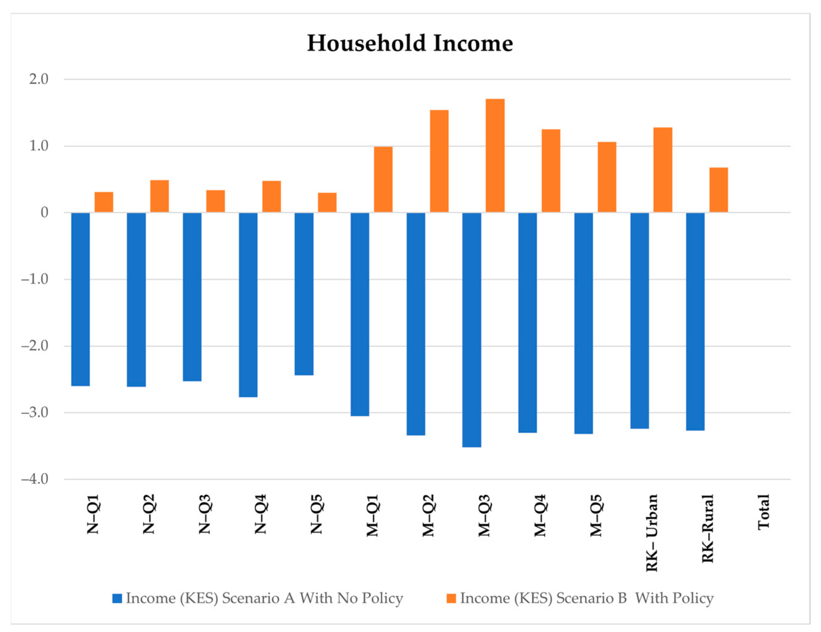
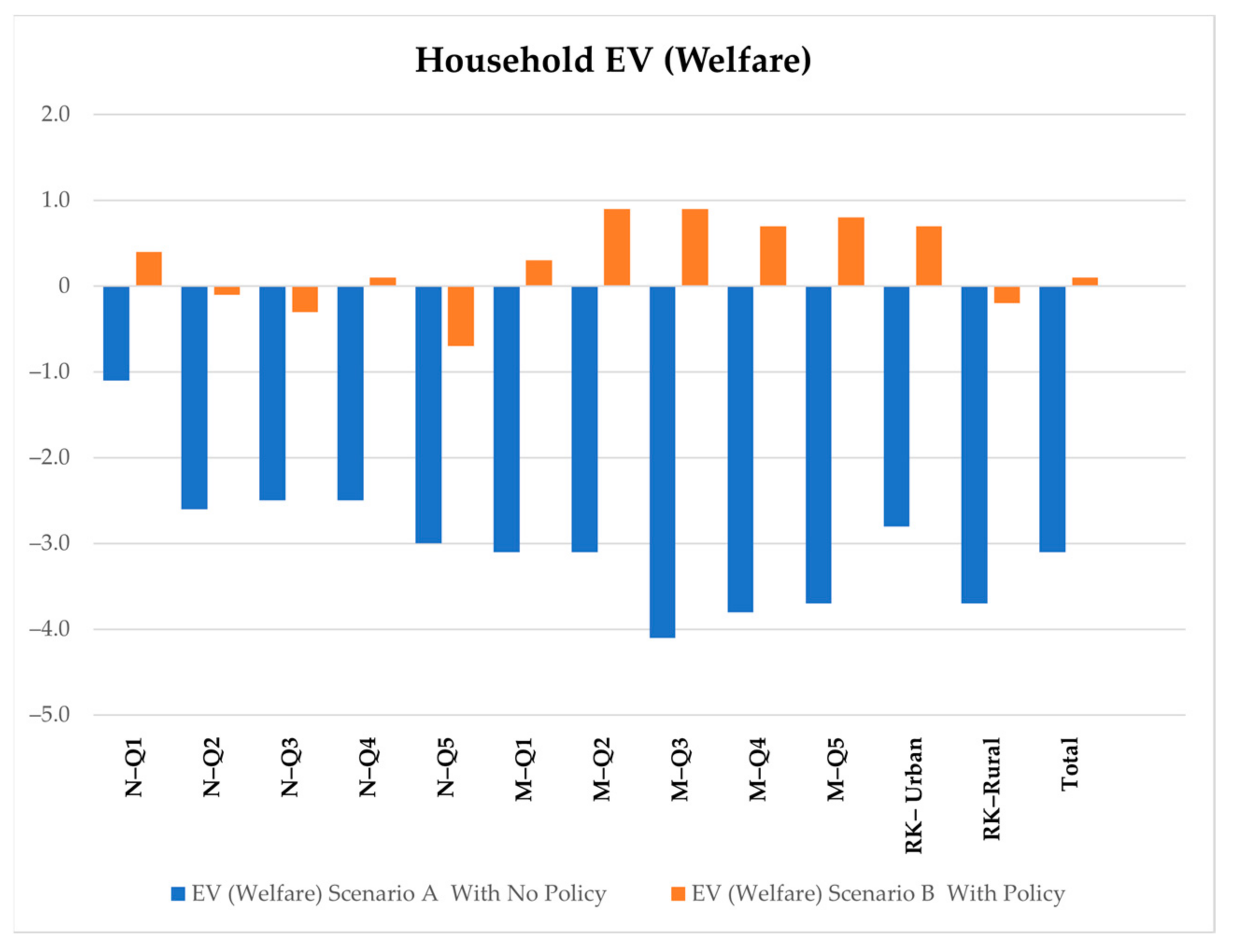
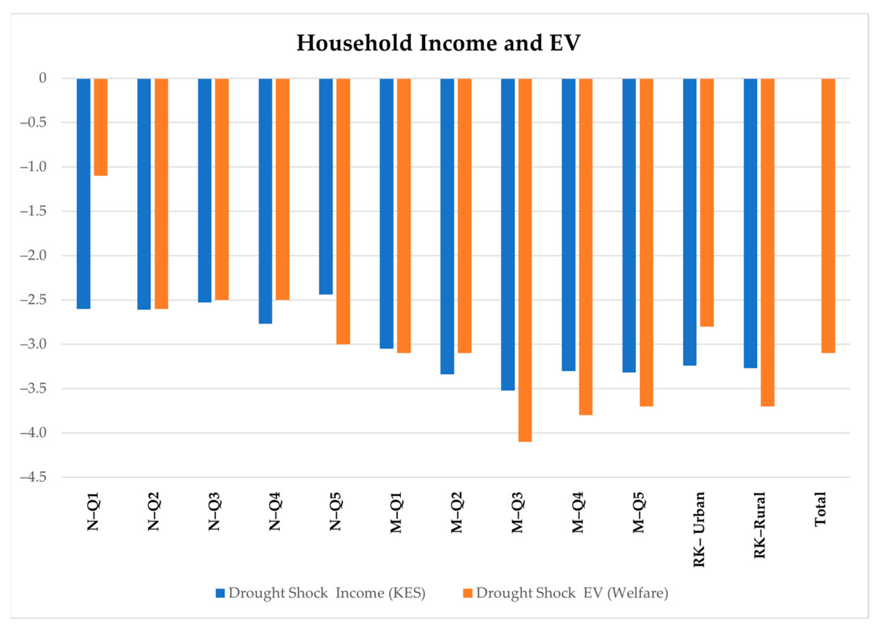
5.1. Drought Mitigation Policy Effectiveness

Based on the mitigation strategies developed in the past by the Kenyan government to handle drought consequences [44,45], this section explores the impact of extending fund transfers to households. Scenario B assumes that the Kenyan government receives financial aid of KES 130 billion (USD 1.16 billion) and transfers to households based on their expenditure losses. This assumption is based on the previous drought mitigation policy implemented by the Kenyan government under drought contingency and the Hunger Safety Net Program for the drought in 2011. Under these programs, the government of Kenya requested USD 1.2 billion from international donors to deal with the negative impact of drought between 2009 and 2011 [46,47]. In the past, the government requested and received the funds based on the estimated damages. To be consistent with this procedure, we assume that the government requests funds based on the economic losses (i.e., damages) due to the reduction in agriculture productivity. Therefore, it is possible to read

Table 3. The number of transfers equals the expenditure loss from the government to the households (scenario A).

Household Units	Transfers from the Government (Billion KES)
Nairobi Quantile 1 (Richest)	13.821
Nairobi Quantile 2	4.93
Nairobi Quantile 3	3.055
Nairobi Quantile 4	2.231
Nairobi Quantile 5 (Poorest)	0.648
Mombasa Quantile 1 (Richest)	2.094
Mombasa Quantile 2	1.363
Mombasa Quantile 3	0.82
Mombasa Quantile 4	0.48
Mombasa Quantile 5 (Poorest)	0.217
Rest of Kenya Urban	24.218
Rest of Kenya Rural	75.258
Total	129.135

from two perspectives: (i) it shows the losses in monetary terms from the households’ point of view, and (ii) it exhibits the number of transfers from the government to the household units. Given the demographic distribution of the Kenyan population, the amount of transfers (i.e., damage suffered) to rural areas is about 58% of the whole available funds of the Kenyan government.

Figure 2 and Figure 3 show the impact of the mitigation policy on households’ income and equivalent variation (EV). Equivalent variation is an index for welfare change due to the consumption price changes, hence, to utility changes. Public transfers increase the total welfare of the households in scenario B (+3.2% than the scenario without policy response). The mitigation policy has redistributive effects on both income and welfare. Indeed, excluding the two major cities, income and welfare in urban areas increased by 4.72% and 3.5%, respectively, whereas in rural communities, income and welfare rose by 3.95% and 3.5%, respectively. Both Figures show improvements in household income and welfare. However, Figure 3 shows that the rural area registers falls in terms of welfare, despite the highest share of transfers from the government to this area (see Table 3). This is mainly because the consumption basket in rural areas highly relies on agrifood commodities, and these areas are most populated compared with urban areas.

Table 4. Percentage change in real GDP and national accounts, scenario A and B.

Real GDP and National Accounts	Drought Shock
	Scenario A, without Policy	Scenario B, with Policy
Absorption	−2.12	0.06
Private consumption	−3.05	0.09
Exports	−2.59	−9.20
Imports	−1.36	2.34
GDP (at market prices)	−2.47	−2.35
Exchange rate	0.93	−5.24

shows the national accounts and impact of drought with or without mitigation policy on indicators, such as total absorption, private consumption, export and import, exchange rate, and GDP. Looking at the aggregate impact of the mitigation policy, Table 4 shows that the total absorption in scenario A shrinks by −2.12%, whereas the policy can fully counterbalance the drought effect (+0.06%). Public transfers positively affect private consumption, which in scenario B increases by +0.09%, whereas in the no-policy scenario, it decreases by −3.05%. The absence/presence of the policy response has substantial effects on the trade balance. In scenario A, the increase in the exchange rate (0.93%) combined with the reduction in household income contracts for both exports (−2.59%) and imports (−1.36%). On the contrary, in scenario B, the Kenyan shilling appreciates by +5.24%, boosting the import (+2.34%) and shrinking the export by −9.20%, worsening the trade balance. The mitigation can only partially offset the negative impact of drought, but it allows for maintaining a higher GDP level than the no-policy scenario (+0.12%).

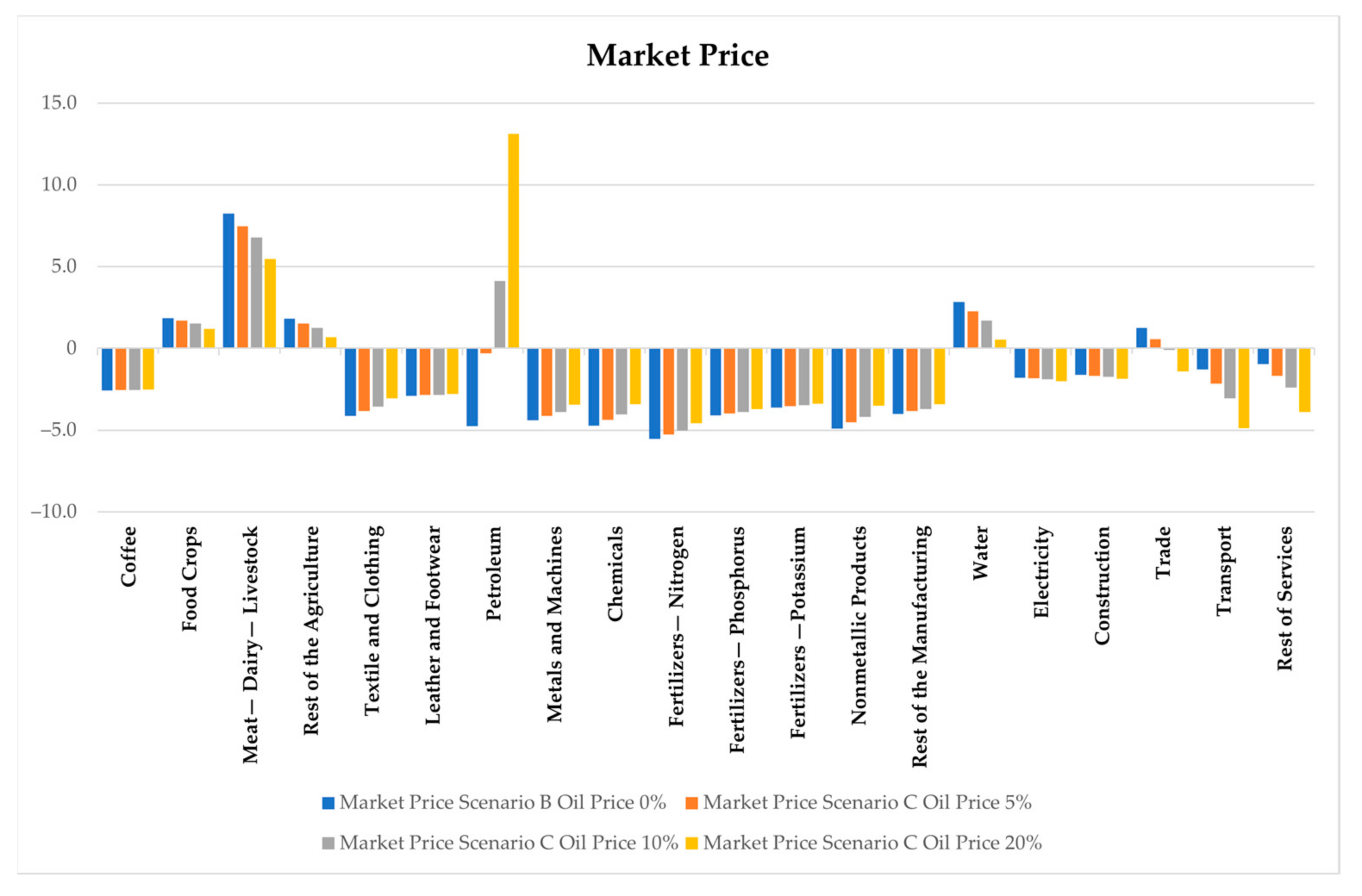
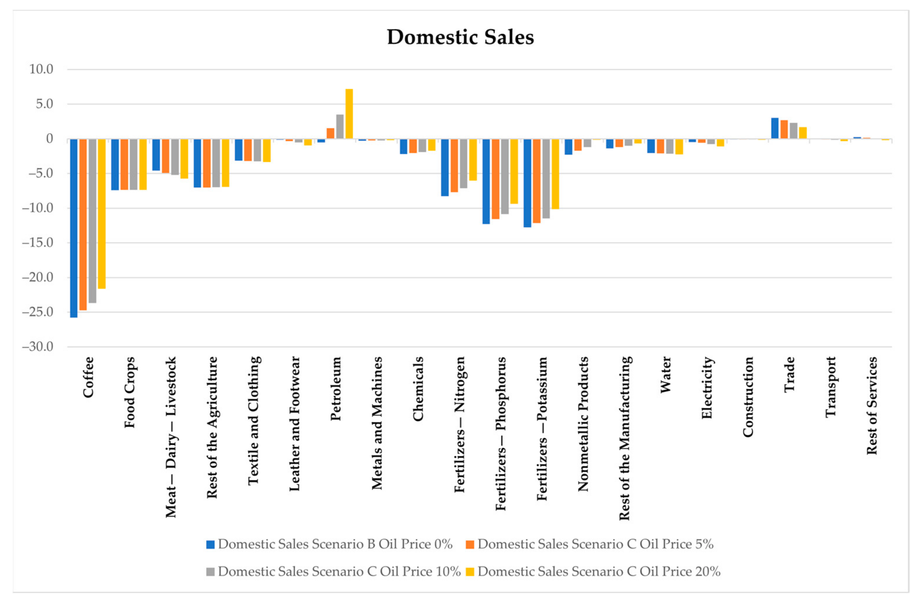
5.2. Oil Shock in the Middle of a Climate Crisis

We conclude our analyses by investigating some scenarios in which, while the government is managing a climate crisis, the economy is hit by an exogenous oil shock, leading to an increase in the oil price. These scenarios are consistent with the double shocks that the Kenyan economy faced in 2014 when the oil price dropped sharply in the second part of the year during a severe drought.

Figure 4 and Figure 5 show the impact of the oil shock in terms of market prices and domestic sales in a scenario where the government is facing a drought. Compared with scenario B (i.e., drought mitigation policy without oil shock), the shocks strongly affect the petroleum price, which increases by 4.45%, 8.88%, and 17.86%, respectively, in the presence of 5%, 10%, and 20% oil shocks. The agricultural industries, particularly those most affected by the drought, register an increase in market prices and a decrease in demand due to production deficiencies. However, by increasing the oil shock (from 0% to 20%), we can see a decreasing trend in agricultural market prices (Figure 4) and an increase in domestic demand (Figure 5). For instance, the growth in the food crops price reduces from +1.85% (in scenario B, i.e., no oil shock) to +1.20% in scenario C with a 20% oil shock. For most of the manufacturing industries, except for “textile and clothing” and “leather and footwear”, the oil shocks increase domestic demands compared with scenario B. The most robust oil price shock produces more pronounced effects in the services industry than in agriculture or manufacturing. Indeed, market prices and domestic sales in services show a downward trend with the increase in oil prices. By increasing the oil prices (i.e., oil shock), the agriculture market prices (such as “food crops” and “meat–dairy–livestock”) show a downward trend, whereas the manufacturing market prices and domestic sales exhibit an increasing trend, as a result of changes in export and import demand. Since Kenya is a net exporter in agrifood industries, a reduction in domestic demand coupled with decreasing market prices during an oil shock can make the export more profitable. To verify this result, we can look at the results of the simulations regarding the trade balance.

Table 5. Percentage change in import and export prices.

Marketed Commodities	Drought Shock Policy and Oil Shock
	Import Quantity				Export Quantity
	Scenario B	Scenario C			Scenario B	Scenario C
	Oil Price +0%	Oil Price +5%	Oil Price +10%	Oil Price +20%	Oil Price 0%	Oil Price +5%	Oil Price +10%	Oil Price +20%
Coffee	−22.72	−21.71	−20.73	−18.73	−29.27	−27.83	−26.42	−23.53
Food crops	15.96	14.33	12.77	9.74	−17.30	−16.50	−15.73	−14.18
Meat–dairy–livestock	19.84	19.02	18.46	17.53	−19.69	−18.75	−17.88	−16.14
Rest of the agriculture	9.90	9.13	8.39	6.91	−16.84	−15.94	−15.07	−13.31
Textile and clothing	1.84	1.22	0.60	−0.65	−10.87	−9.94	−9.07	−7.29
Leather and footwear	−0.18	−0.37	−0.60	−1.04	−4.88	−4.21	−3.58	−2.38
Petroleum	1.05	−0.83	−2.59	−5.61	−3.20	−4.98	−6.82	−10.62
Metals and machines	−2.69	−2.32	−1.99	−1.36	−1.46	−1.10	−0.75	−0.02
Chemicals	0.48	0.04	−0.41	−1.35	−5.98	−5.03	−4.13	−2.27
Fertilizers—nitrogen	−11.18	−11.17	−11.16	−11.16	−5.01	−3.51	−2.03	1.05
Fertilizers—phosphorus	−10.65	−10.69	−10.73	−10.82	−15.59	−13.68	−11.78	−7.80
Fertilizers—potassium	−10.40	−10.43	−10.47	−10.55	−17.34	−15.55	−13.79	−10.09
Nonmetallic products	−1.01	−0.89	−0.78	−0.58	−4.27	−3.11	−1.97	0.40
Rest of manufacturing	1.03	0.57	0.11	−0.82	−5.40	−4.22	−3.07	−0.70
Water	0.00	0.00	0.00	0.00	0.00	0.00	0.00	0.00
Electricity	0.00	0.00	0.00	0.00	0.00	0.00	0.00	0.00
Construction	0.00	0.00	0.00	0.00	0.00	0.00	0.00	0.00
Trade	6.53	5.53	4.60	2.79	−0.35	−0.11	0.11	0.60
Transport	2.13	1.34	0.56	−1.05	−2.13	−1.49	−0.86	0.43
Rest of services	2.53	1.80	1.09	−0.37	−1.97	−1.46	−0.97	0.02

shows the drought policy’s impact on trade with and without oil price shocks. In terms of imports of agricultural products, the scenario without oil shock (scenario B) shows a more significant increase for most productions than the scenario with a double shock. As the oil price increases, agricultural commodities show a decreasing trend in imports and an increasing trend in exports. On the one hand, these dynamics are in line with the reduction of the agricultural, domestic sales for agricultural commodities (see Figure 5). The increase in the price of oil and raw materials used in the production process negatively affects the purchasing power of the households (particularly, fertilizers for agriculture production show the increasing prices with oil shocks in Table 5). However, the growth in the price of these intermediate goods leads to an increase in the price of agricultural commodities, positively affecting the profitability of agriculture commodity export during the oil shock. Moreover, the increase in the world oil price reduces petroleum imports and most manufacturing commodities. Finally, fertilizers registered the highest reduction in either import or export quantity regardless of oil prices. This may be due to the agricultural industry’s significant decrease in production during the drought shock. The trend of increasing exports of agricultural commodities can be explained by the development of domestic sales and market prices (see Figure 4 and Figure 5). While domestic demand for agrifood products decreases during the oil shock due to the reduction in the purchasing power of domestic consumers, the reduction in domestic product prices may lead to an increase in export products. Therefore, domestic suppliers are more likely to export their products in order to sell them to the external market at relatively higher prices than in the domestic market.

Figure 6 and Figure 7 show the impact of oil shocks on the effectiveness of the drought mitigation policy in terms of household’s income and EV (welfare). In terms of household’s income (Figure 6), the oil shock erodes the positive effects of the drought mitigation policy (scenario B). Nevertheless, with a +5% oil price shock, other parts of the country still can benefit from the drought mitigation policy except for Nairobi household units. The reduction in household income in Nairobi is mainly because, according to the data, workers from Nairobi are employed more in the oil-related industries, such as those that deal with petroleum production, chemicals, and fertilizers. Looking at the income changes in the two main cities, Figure 6 shows that the average reduction in the first two richest quintiles (Q1 and Q2) is lower than in the two lowest income quantiles (Q4 and Q5). These findings confirm the results of scenario B, according to which richer quantiles experience more remarkable improvement due to government transfers. These results can be explained by the mitigation policy design, which allocates many transfers to the first two quantiles in both cities. Having a higher income/wealth level, richer quantiles register more significant losses in absolute terms due to drought. Then, according to the mitigation policy, they will receive more transfers. This will result in lower losses for these quantiles than for poorer ones, with regressive consequences on income/wealth distribution. Comparing the results between urban and rural areas in both scenarios, even if rural communities receive a higher number of transfers, they will register lower net benefits than urban communities. All these results are confirmed in sign and even more so in magnitude regarding welfare (Figure 7).

Table 6. Percentage change in real GDP and national accounts, scenarios B and C.

Real GDP and National Accounts	Drought Shock Policy and Oil Shock
	Scenario B	Scenario C
	Oil Price +0%	Oil Price +5%	Oil Price +10%	Oil Price +20%
Absorption	0.06	−0.31	−0.68	−1.40
Private consumption	0.09	−0.45	−0.98	−2.00
Exports	−9.20	−8.49	−7.81	−6.43
Imports	2.34	1.50	0.70	−0.77
GDP (at market prices)	−2.35	−2.38	−2.42	−2.50
Exchange rate	−5.24	−4.78	−4.36	−3.5

contains total absorption, private consumption, overall export and import, exchange rate, and GDP. This table shows the negative impact of the oil shock on the main aggregate variables. For example, the most potent oil shock reduces the total absorption and private consumption by 1.46% and 2.09%, compared with the scenario with no oil price increase. In terms of trade, the imports show a reduction in the oil price shock, from a growth of 2.34% in the scenario without shock to a decrease of −0.77% in the worst scenario C (+20% oil price). On the other hand, exports increased by 2.77% in the +20% oil price shock scenario compared to scenario B.

Finally, the oil price shock negatively affects the GDP, which in the worst scenario registers a further decline by 7.959 billion KES (−0.15%) compared to scenario B.

6. Conclusions and Remarks

Global climate change and the continuous depletion of nonrenewable natural resources may lead to a future characterized by a higher frequency of extreme climate events (i.e., floods, hurricanes, or droughts) and resource supply shocks (i.e., oil price shocks). Sub-Saharan African countries are already particularly exposed to these types of shocks because of both their socioeconomic conditions and geographical conformation.

This article presents a static CGE model applied to Kenya to investigate the effectiveness of a mitigation policy (transfers to the population) in managing a climate crisis (i.e., a drought) whose effect may be exacerbated by a contemporaneous exogenous oil price shock. This scenario is coherent with what happened in 2014 when the price of oil dropped sharply by 30% during a severe drought.

To address the redistributive implications of the shocks and the mitigation policy, we estimate the Fisher parameter [36] for each household quantile using the method introduced by [37]. We assume a range of oil shocks that lead to a jump in world oil prices by different magnitudes (+5%, +10%, and +20%). In contrast, the drought strongly affects agricultural production, shrinking the average output by 10%. Based on the past postdrought strategies of the Kenyan government, the climate crisis mitigation policy implemented by the government consists of externally financed transfers to households.

The analysis shows that public transfers are an effective tool for mitigating drought effects, improving welfare and GDP in the short run (+3.2% and +0.12%, respectively) compared with the scenario without postdrought policy. Looking at the effectiveness of the mitigation policy in terms of income variation at the household level, the model suggests that transfers positively affect both the two richer quantiles and the middle-lower quantiles with comparable magnitude in the two main cities. In contrast, they have a more substantial impact on urban than rural communities.

However, implementing this mitigation policy to manage drought during an oil crisis may have regressive effects on the population and negatively impact the overall economy. Results of the analysis suggest that, in the domestic market, an increasing trend in oil prices with existing drought mitigation policy leads to a decreasing trend in market prices and a rising trend in domestic sales for agriculture and manufacturing industries. In terms of trade, imports show a downward trend in agriculture compared with an upward trend in exports. Considering that Kenya is a net exporter of agricultural commodities, this means that despite more expensive oil prices, exports can become more profitable for agriculture industries.

Regarding household income and welfare, our findings suggest a regressive impact of oil shocks on drought mitigation policy. Indeed, comparing the two extreme quantiles (richest and poorest), the wealthiest quantile always registers a lower reduction in income and welfare than the poorest quantile when a climate crisis is coupled with an oil shock. The explanation of this result is the design of the mitigation policy, which allocates a higher number of transfers from the government to the richer quantiles since they register a more substantial reduction in expenditure (in absolute terms).

In conclusion, mitigation policy effectiveness can be strongly affected by the complex interaction between drought and oil shocks, and public authorities should pay attention to this in policy implementation. Our study shows that the complexity of policy implementation is highly related to the levels of contemporaneous shocks. On the other hand, these findings call for a new scheme of transfer allocation, in which rural and low-income household quintiles should receive more attention from mitigation policy in the postdrought period, as they are the most vulnerable to external shocks.

References

1. Geda, A. The Historical Origin of the African Economic Crisis: From Colonialism to China; Cambridge Scholars Publishing: Newcastle upon Tyne, UK, 2019. [Google Scholar]
2. Calvo, C.; Dercon, S. Measuring Individual Vulnerability; Discussion Paper No. 229; University of Oxford: Oxford, UK, 2005. [Google Scholar]
3. Shepherd, A.; Mitchell, T.; Lewis, K.; Lenhardt, A.; Jones, L.; Scott, L.; Muir-Wood, R. The Geography of Poverty, Disasters and Climate Extremes in 2030; ODI Report; ODI: London, UK, 2013. [Google Scholar]
4. Pradhan, K.C.; Mukherjee, S. Covariate and idiosyncratic shocks and coping strategies for poor and non-poor rural households in India. J. Quant. Econ. 2018, 16, 101–127. [Google Scholar] [CrossRef]
5. Bazzana, D.; Foltz, J.; Zhang, Y. Impact of climate smart agriculture on food security: An agent-based analysis. Food Policy 2022, 111, 102304. [Google Scholar] [CrossRef]
6. Njoka, J.T.; Yanda, P.; Maganga, F.; Liwenga, E.; Kateka, A.; Henku, A.; Mabhuye, E.; Malik, N.; Bavo, C. Kenya: Country Situation Assessment. 2016. Available online: https://idl-bncidrc.dspacedirect.org/bitstream/handle/10625/58566/IDL-58566.pdf (accessed on 2 July 2022).
7. UNEP and the Government of Kenya. Kenya Drought: Impacts on Agriculture, Lifestock and Wildlife; UNEP and the Government of Kenya: Nairobi, Kenya, 2006. [Google Scholar]
8. Huho, J.M.; Mugalavai, E.M. The Effects of Droughts on Food Security in Kenya. Int. J. Clim. Chang. Impacts Responses 2010, 2, 61–72. [Google Scholar] [CrossRef]
9. Government of the Republic of Kenya. Kenya Post-Disaster Needs Assessment (PDNA) 2008–2011 Drought. 2012. Available online: https://www.gfdrr.org/sites/default/files/publication/pda-2011-kenya.pdf (accessed on 2 July 2022).
10. Hamilton, J.D. Historical Oil Shocks. In Routledge Handbook of Major Events in Economic History; Parker, R.E., Whaples, R., Eds.; Routledge Taylor and Francis Group: New York, NY, USA, 2013; pp. 239–265. [Google Scholar]
11. Odhiambo, N.M.; Nyasha, S. Oil price and economic growth in Kenya: A trivariate simulation. Int. J. Sustain. Energy Plan. Manag. 2019, 19, 3–12. [Google Scholar] [CrossRef]
12. World Bank Group. Commodity Markets Outlook: Urbanization and Commodity Demand, October 2021; World Bank: Washington, DC, USA, 2021. [Google Scholar]
13. EPRA. ENERGY & PETROLEUM STATISTICS REPORT 2019. Available online: https://www.epra.go.ke/wp-content/uploads/2020/09/Energy-and-Petroleum-Statistics-Report-2019-1.pdf (accessed on 2 July 2022).
14. Hamilton, J.D. This is what happened to the oil price-macroeconomy relationship. J. Monet. Econ. 1996, 38, 215–220. [Google Scholar] [CrossRef]
15. Berument, M.H.; Ceylan, N.B.; Dogan, N. The Impact of Oil Price Shocks on the Economic Growth of Selected MENA Countries. Energy J. 2010, 31, 149–176. Available online: http://www.jstor.org/stable/41323274 (accessed on 2 July 2022).
16. Mainar Causapé, A.J.; Boulanger, P.; Dudu, H.; Ferrari, E.; McDonald, S.; Caivano, A. Social Accounting Matrix of Kenya 2014; Publications Office of the European Union: Seville, Spain, 2018. [Google Scholar]
17. Narayan, P.K. Macroeconomic impact of natural disasters on a small island economy: Evidence from a CGE model. Appl. Econ. Lett. 2003, 10, 721–723. [Google Scholar] [CrossRef]
18. Zhou, L.; Chen, Z. Are CGE models reliable for disaster impact analyses? Econ. Syst. Res. 2021, 33, 20–46. [Google Scholar] [CrossRef]
19. Arndt, C.; Tarp, F. Who gets the goods? A general equilibrium perspective on food aid in Mozambique. Food Policy 2001, 26, 107–119. [Google Scholar] [CrossRef]
20. Juana, J.S.; Makepe, P.M.; Mangadi, K.T.; Narayana, N. The Socio-economic Impact of Drought in Botswana. Int. J. Environ. Dev. 2014, 11, 43–60. [Google Scholar]
21. Borgomeo, E.; Vadheim, B.; Woldeyes, F.B.; Alamirew, T.; Tamru, S.; Charles, K.J.; Kebede, S.; Walker, O. The Distributional and Multi-Sectoral Impacts of Rainfall Shocks: Evidence from Computable General Equilibrium Modelling for the Awash Basin, Ethiopia. Ecol. Econ. 2018, 146, 621–632. [Google Scholar] [CrossRef]
22. Kilimani, N.; Van Heerden, J.H.; Bohlmann, H.; Roos, L. Economy-wide impact of drought induced productivity losses. Disaster Prev. Manag. Int. J. 2018, 27, 636–648. [Google Scholar] [CrossRef]
23. Gebreegziabher, Z.; Stage, J.; Mekonnen, A.; Alemu, A. Climate change and the Ethiopian economy: A CGE analysis. Environ. Dev. Econ. 2016, 21, 205–225. [Google Scholar] [CrossRef]
24. Ntombela, S.M.; Nyhodo, B.; Ngqangweni, S.; Phahlane, H.; Lubinga, M.H. Economy-wide effects of drought on South African Agriculture: A computable general equilibrium (CGE) analysis. J. Dev. Agric. Econ. 2017, 9, 46–56. [Google Scholar]
25. Manuel, L.; Chiziane, O.; Mandhlate, G.; Hartley, F.; Tostão, E. Impact of climate change on the agriculture sector and household welfare in Mozambique: An analysis based on a dynamic computable general equilibrium model. Clim. Chang. 2021, 6, 167. [Google Scholar] [CrossRef]
26. Hatibu, H.; Semboja, H. The effects of energy taxes on the Kenyan economy: A CGE analysis. Energy Econ. 1994, 16, 205–215. [Google Scholar] [CrossRef]
27. Sánchez, M.V. Welfare Effects of Rising Oil Prices In Oil-Importing Developing Countries. Dev. Econ. 2011, 49, 321–346. [Google Scholar] [CrossRef]
28. Pradhan, B.K.; Sahoo, A. Oil Price Shocks and Poverty in a CGE Framework. In Proceedings of the MIMAP Training Program, Manila, Philippines, 28 February–9 March 2000. [Google Scholar]
29. Solaymani, S.; Yusof, N.Y.B.M.; Yavari, A. The role of government climate policy in an oil price shock: A CGE simulation analysis. In Proceedings of the 2015 International Conference on Modeling, Simulation and Applied Mathematics, Phuket, Thailand, 23–24 August 2015; pp. 260–263. [Google Scholar]
30. Gershon, O.; Ezenwa, N.E.; Osabohien, R. Implications of oil price shocks on net oil-importing African countries. Heliyon 2019, 5, 02208. [Google Scholar] [CrossRef]
31. Bekhet, H.A.; Yusop, N.Y.M. Assessing the relationship between oil prices, energy consumption and macroeconomic performance in Malaysia: Co-integration and vector error correction model (VECM) approach. Int. Bus. Res. 2009, 2, 152–175. [Google Scholar] [CrossRef]
32. Yildirim, Z.; Arifli, A. Oil price shocks, exchange rate and macroeconomic fluctuations in a small oil-exporting economy. Energy 2021, 219, 119527. [Google Scholar] [CrossRef]
33. Kamasa, K.; Amponsah, B.D.; Forson, P. Do Crude Oil Price Changes Affect Economic Welfare? Empirical Evidence from Ghana. Ghana Min. J. 2020, 20, 51–58. [Google Scholar]
34. Robinson, S.; Yúnez-Naude, A.; Hinojosa-Ojeda, R.; Lewis, J.D.; Devarajan, S. From stylized to applied models: Building multisector CGE models for policy analysis. N. Am. J. Econ. Financ. 1999, 10, 5–38. [Google Scholar] [CrossRef]
35. Löfgren, H. External Shocks and Domestic Poverty Alleviation: Simulation with a CGE Model of Malawi; 1043 TMD Discussion Paper 71; International Food Policy Research Institute: Washington, WA, USA, 2001. [Google Scholar]
36. Frisch, R. A complete scheme for computing all direct and cross elasticities in a model with many sectors. Econometrica 1959, 27, 177–196. [Google Scholar] [CrossRef]
37. Lluch, C. Consumer Demand Functions, Spain, 1958–1964. Eur. Econ. Rev. 1971, 2, 277–302. [Google Scholar] [CrossRef]
38. Vigani, M.; Dudu, H.; Ferrari, E.; Causape, A.M. Estimation of Food Demand Parameters in Kenya. A Quadratic Almost Ideal Demand System (QUAIDS) Approach; EUR 29657 EN; PUBSY No. JRC115472; Publications Office of the European Union: Luxembourg, 2019; ISBN 978-92-76-00025-9. [Google Scholar] [CrossRef]
39. Aragie, E.A.; McDonald, S. Semi-subsistence farm households and their implications for policy response. In Proceedings of the 17th Annual Conference on Global Economic Analysis, Dakar, Senegal, 18–20 June 2014. [Google Scholar]
40. Dupuy, A. Hicks Neutral Technical Change Revisited: CES Production Function and Information of General Order. Top. Macroecon. 2006, 6. [Google Scholar] [CrossRef]
41. McDonald, S. Drought in Southern Africa: A study for Botswana. In Proceedings of the XIII International Conference on Input-Output Techniques, Macerata, Italy, 21–25 August 2000. [Google Scholar]
42. Hertel, T.W.; Burke, M.B.; Lobell, D.B. The poverty implications of climate-induced crop yield changes by 2030. Glob. Environ. Chang. 2010, 20, 577–585. [Google Scholar] [CrossRef]
43. Tebaldi, C.; Lobell, D.B. Towards probabilistic projections of climate change impacts on global crop yields. Geophys. Res. Lett. 2008, 35, L08705. [Google Scholar] [CrossRef]
44. Republic of Kenya. Sector Plan for Drought Risk Management and Ending Drought Emergencies; Republic of Kenya: Nairobi, Kenya, 2014; Available online: http://www.alnap.org/help-library/sector-plan-for-droughtrisk-management-and-ending-drought-emergencies (accessed on 2 July 2022).
45. Republic of Kenya. National Drought Early Warning Bulletin for December; Republic of Kenya: Nairobi, Kenya, 2016; Available online: http://www.alnap.org/help-library/national-drought-early-warning-bulletin-fordecember (accessed on 2 July 2022).
46. Fitzgibbon, C. Shock-Responsive Social Protection in Practice: Kenya’s Experience in Scaling Up Cash Transfers. Humanitarian Policy; HPN/ODI: London, UK, 2016; Available online: http://www.alnap.org/help-library/shock-responsive-social-protection-in-practice-kenya%E2%80%99sexperience-in-scaling-up-cash (accessed on 2 July 2022).
47. Obrecht, A. Adapting According to Plan: Early Action and Adaptive Drought Response in Kenya; ALNAP Country Study; ODI/ALNAP: London, UK, 2019. [Google Scholar]
48. Blonigen, B.A.; Flynn, J.E.; Reinert, K.A. Sector-Focused General Equilibrium Modeling, in Applied Methods of Trade Policy Analysis: A Handbook; Francois, J.F., Reinert, K.A., Eds.; Cambridge University Press: Cambridge, UK, 1997; pp. 189–230. [Google Scholar]
49. Johansen, L. A Multi-Sectoral Study of Economic Growth; North-Holland Publishing Co.: Amsterdam, The Netherland, 1960. [Google Scholar]
50. Rattsø, J. Different macroclosures of the original Johansen model and their impact on policy evaluation. J. Policy Model. 1982, 4, 85–97. [Google Scholar] [CrossRef]
Figure 1. The output production process in the CGE model for Kenya.
Sustainability 14 11273 g001
Figure 2. Percentage change in household’s income. Scenario A (drought) in blue and scenario B (drought with policy response) in orange. N means Nairobi, M refers to Mombasa, whereas RK describes the rest of Kenya. The households in Nairobi and Mombasa are divided in quantile, from the richest (Q1) to the poorest (Q5). (For interpretation of the references to color in the figure legend, the reader is referred to the web version of this article.).
Sustainability 14 11273 g002
Figure 3. Percentage change in household’s EV (welfare). Scenario A (drought) in blue and scenario B (drought with policy response) in orange. N means Nairobi, M refers to Mombasa, whereas RK describes the rest of Kenya. The households in Nairobi and Mombasa are divided in quantile, from the richest (Q1) to the poorest (Q5).
Sustainability 14 11273 g003
Figure 4. Percentage change in market prices, scenario B (drought with policy response) and scenario C (drought with policy and oil shock).
Sustainability 14 11273 g004
Figure 5. Percentage change in domestic sales, scenario B (drought with policy response) and scenario C (drought with policy and oil shock).
Sustainability 14 11273 g005
Figure 6. Percentage change in household income, scenario B (drought with policy response) and scenario C (drought with policy and oil shock). N means Nairobi, M refers to Mombasa, whereas RK describes the rest of Kenya. The households in Nairobi and Mombasa are divided in quantile, from the richest (Q1) to the poorest (Q5).
Sustainability 14 11273 g006
Figure 7. Percentage change in household’s EV (welfare), scenario B (drought with policy response) and scenario C (drought with policy and oil shock). N means Nairobi, M refers to Mombasa, whereas RK describes the rest of Kenya. The households in Nairobi and Mombasa are divided in quantile, from the richest (Q1) to the poorest (Q5).
Sustainability 14 11273 g007