Fiscal Decentralization, Local Government Behavior, and Macroeconomic Effects of Environmental Policy

Abstract

With the rapid economic growth, environmental problems have become a significant bottleneck restricting the high-quality development of China’s economy. In the fiscal decentralization system, balancing economic growth and environmental governance is an issue that needs to be paid attention to in fiscal policy. This paper studies the impact of fiscal decentralization on the environmental policy in China. We incorporate the central and local government structure into a standard environmental dynamic stochastic general equilibrium (E-DSGE) model. The economy was featured with multiple-level governments where the local governments implement fiscal policies through the trade-off between pursuing economic growth and environmental governance. The results indicate that implementing a carbon emission tax is not conducive to economic growth but helps reduce environmental pollution. Second, deepening fiscal decentralization has heterogeneous effects on central and local fiscal expenditures. Deepening fiscal decentralization strengthens the positive externality of local government expenditures to output, but it also leads to further deterioration of environmental pollution. The positive externality of the central government expenditures will weaken with the increase in fiscal decentralization, but it is conducive to improving the quality of the environment. Third, deepening fiscal decentralization is conducive to improving social welfare and alleviating environmental pollution. If the local government fiscal expenditures are biased toward environmental governance expenditures, this is beneficial to improve social welfare and the quality of the environment.

1. Introduction

With the rapid economic growth, environmental problems have become a significant bottleneck restricting the high-quality development of China’s economy. In January 2018, China levied environmental protection tax, implemented a dynamic tax amount mechanism, and incorporated it into local fiscal revenue. In July 2021, China’s carbon market officially launched online trading. The market mechanism has achieved initial results in controlling and reducing greenhouse gas emissions and the cost of carbon emissions. Liu et al. [1] argue that levying a carbon tax prefers to reduce CO₂ emissions as well as restrain economic growth. Zhang [2] believes that the carbon tax is seen as an essential policy tool to influence the sustainability. Cao et al. [3] find that the 2030 carbon peaking target for China are easily met, but the 2060 carbon neutrality goal cannot be achieved even with our highest carbon tax rates. For environmental policy, existing studies have expanded from economic reasons to institutional factors and government behavior. At the same time, fiscal decentralization is a necessary institutional arrangement that affects the supply of public goods such as the environment. It is of great theoretical and practical significance to explore what effect fiscal decentralization has on environmental pollution and how to stimulate the subjective initiative of local governments in ecological governance under the fiscal decentralization system.

China’s environmental policy has adopted the mode of dual governance at the central and local governments under the fiscal decentralization and the performance appraisal system centered on GDP. On the one hand, local government officials have a strong will to pursue economic growth subjectively, and they regard promoting regional economic growth as their primary goal during their term of office. However, improving environmental quality cannot bring about economic and political performance in the short run. It also reflects that limited financial funds will be occupied due to the “crowding out effect”. This will guide local financial expenditures to be more inclined to non-environmental governance expenditures (NEGE), while environmental governance expenditures (EGE) are insufficient. On the other hand, due to the mismatch between local government financial rights and administrative powers, increasing EGE will increase local financial pressures, resulting in local governments lacking enthusiasm and initiative in the supply of public goods such as the environment, thus deteriorating regional environmental quality. It shows that under the fiscal decentralization model, the central government and the local government have both political decision-making conflicts and economic interests’ competition in the trade-off between economic growth and environmental quality. Although they are both “regulators”, their interest demands are different.

This paper seeks to understand the impact of fiscal decentralization on environmental pollution. To this end, we formulate a E-DSGE model embodying the central and local government structure. The model that we construct has three key features. First, we incorporate the central and local government structure into a standard E-DSGE model, where the local governments implement fiscal policies through the trade-off between pursuing economic growth and environmental governance. Second, in the utility function, we consider the negative impact of environmental pollution on the utility of the representative household, and we introduce different taxes, such as carbon emission tax, consumption tax, capital income tax, and labor income tax. Third, in the production function, we introduce a positive externality of NEGE on output. The fiscal expenditure decentralization degree and the fiscal revenue decentralization degree are described in the production function and the dynamic accumulation equation of environmental pollution, respectively. In this way, we explore how the central government influences the behavior of local governments and the motivation behind the preference for NEGE, and the macroeconomic effects of environmental policies under the fiscal decentralization system.

The structure of this paper is as follows. Section 2 presents the related literature. Section 3 describes the structure of the E-DSGE model of multi-level governments. Section 4 shows the parameter estimation. Section 5 carries out the simulation and welfare analysis. Section 6 summarizes the main results and policy implications.

2. Literature Review

Some theoretical and empirical studies have deeply analyzed the impact of fiscal decentralization on environmental quality, but they have not reached a consistent conclusion. Glazer [4] and Levinson [5] find that fiscal decentralization improves environmental quality. When the local government realizes that the improvement of environmental quality is an essential part of resident’s welfare, the local government may adopt stricter environmental standards to promote the progress of the local environmental quality while promoting regional economic development. Tiebout [6] and Stigler [7] believe that the government assumes the responsibility for environmental protection; to attract residents and resources to flow into its jurisdiction, fiscal decentralization can effectively motivate local governments to provide high-level environmental quality and other public service expenditures. Therefore, fiscal decentralization is conducive to the improvement of environmental quality. Hayek [8] and Silva [9] find that local governments have advantages in obtaining information and understanding the preferences and needs of residents; local environmental policies are more conducive to improving environmental quality. Khan et al. [10] investigate the impact of fiscal decentralization on CO₂ emissions by using a balanced panel dataset of seven OECD countries, and show that fiscal decentralization improves environmental quality. Chen, Xu, and Qi [11] investigate the causal effects of environmental decentralization on local governments’ environmental governance. They present strong evidence that establishing the Supervision Centers for Environmental Protection significantly prompt firms to reduce emission pollution. Meng et al. [12] examine the asymmetric link between fiscal decentralization, environmental innovation, and carbon emissions in highly decentralized countries. They show that fiscal decentralization significantly mitigates carbon emissions only at lower to medium emissions quantiles. Other studies believe that fiscal decentralization reduces the quality of the environment. Under the fiscal decentralization system, local governments compete to develop the local economy, attract investment, increase employment opportunities or tax revenue, and relax environmental supervision. Under low-standard environmental constraints, pollution cannot be effectively controlled, leading to the deterioration of environmental quality [13,14,15,16,17]. Zeng et al. [18] find that fiscal decentralization in China provides local governments with incentives for the development of high pollution industries and of large state-owned enterprises, which is not conducive to the improvement of environmental quality. Xia et al. [19] use the Spatial Durbin Model analyzing the spatial impact of fiscal decentralization on regional carbon emissions. They find that fiscal decentralization, both within the region and in its neighborhood, will contribute to carbon emissions in the region. Environmental decentralization will help reduce carbon emissions, while environmental decentralization in neighboring regions will increase carbon emissions in the region.

Recent studies discuss environmental issues using macroeconomic approaches, especially the DSGE model. The work of Heutel [20] is the first study that use a DSGE model that includes a pollution externality in studying environmental issues. He finds that optimal policy allows carbon emissions to be procyclical. However, optimal policy dampens the procyclicality of emissions compared to the unregulated case. Annicchiarico and Di Dio [21] present a New Keynesian DSGE model embodying pollutant emissions and environmental policy. They analyze the performance of alternative environmental policy rules under real and nominal uncertainty and find the optimal policy response to inflation. They find that an emissions cap policy is likely to dampen macroeconomic fluctuations, and the optimal environmental policy response to shocks is strongly influenced by the degree to which prices adjust and by the monetary policy reaction. Hao et al. [22] develop a neoclassical model investigate the impact of fiscal decentralization on environmental quality, and they show that there exists an inverted-U shaped relationship between fiscal decentralization and GDP per capita. Ying [23] compares the effectiveness of standard macroeconomic tools (fiscal and monetary policies) with carbon taxation in curbing air pollution by using an E-DSGE model. They find that while all the aforementioned policies could stabilize carbon emissions, their underlying mechanisms are different.

There is no unified consensus on the impact of fiscal decentralization on the ecological environment, mainly due to different theoretical or empirical model frameworks with limited explanatory power. At the same time, most studies do not have an in-depth discussion on the structure of government spending under fiscal decentralization, and few studies involve the analysis of tax distortions, only considering the average tax rate. In addition, few studies have made an in-depth analysis of how the central government affects the behavior of local governments, which, in turn, affects the effect of environmental governance in fiscal decentralization.

3. Multi-Level-Government E-DSGE Model

We construct a multi-level-government E-DSGE model. The model considers a closed economy consisting of representative households, firms, multi-level governments, and the central bank. The economy presents: (i) households maximize their utility by consuming, offering labor, leasing capital to firms, and purchasing central and local government bonds; (ii) there are two types of firms in the economy. One is the perfectly competitive final goods firms, and the other is the monopolistic competition intermediate goods firms; (iii) the central and local government’s expenditures are financed by taxation and the issuance of government bonds, and the government is taxed at a proportional tax rate that is shared proportionally between the central and local governments; (iv) the central bank implements monetary policy by adjusting the nominal interest rates based on the output and inflation deviate from their steady-state values.

3.1. Household

We assume that there is a continuous set of representative households in the economy whose behavior is not only affected by income and asset accumulation but also by the degree of environmental pollution $M_t$. A representative infinitely lived household maximizes his lifetime utility by choosing consumption $C_t$, labor supply $N_t$, central government bond holdings $B_t^C$, local government bond holdings $B_t^L$, capital $K_t$, and investment $I_t$.

$$E_t{\displaystyle \sum _{t=0}^{\propto }{\beta }^t}\left(\ln C_t-{\mu }_N\frac{N_t^{1+\eta }}{1+\eta }-\ln M_t\right)$$

The budget constraint for a representative household is given by

$$P_t{C}_t\left(1+{\tau }_t^C\right)+P_t{I}_t+B_{t+1}^C+B_{t+1}^L=P_t{r}_t^K{K}_t\left(1-{\tau }_t^K\right)+P_t{w}_t{N}_t\left(1-{\tau }_t^N\right)+R_{t-1}^C{B}_t^C+R_{t-1}^L{B}_t^L$$

(1)

where $\beta$ is the discount factor, $\eta$ represents the inverse elasticity of labor supply, ${\tau }_t^C$, ${\tau }_t^K$ and ${\tau }_t^N$ denotes consumption tax rate, capital tax rate, and labor income tax rate, respectively, $w_t$ and $r_t^K$ is wage and capital rent, $R_t$ denotes the nominal interest rate, $R_t^C$ is the nominal return rate of central government bonds, and $R_t^L$ denotes the nominal return rate of local government bonds.

The low of motion of the capital is given by

$$K_{t+1}=\left(1-\delta \right)K_t+I_t\left[1-s\left(\frac{I_t}{I_{t-1}}\right)\right]$$

(2)

where $\delta$ is the depreciation rate of capital. According to Christiano et al. [24], the investment adjustment cost function $s_t(\cdot )$ is set as follows.

$$s\left(x\right)=\frac{1}{2}\left[e^{\sqrt{s^{″}}\left(x-1\right)}+e^{-\sqrt{s^{\prime }}\left(x-1\right)}-2\right]$$

(3)

where ${\sigma }_a$ and ${\sigma }_b$ are the parameters.

3.2. Firms

A perfectly competitive final good firm uses the intermediate goods $Y_{j,t}$ as an input factor with the price $P_{j,t}$ to produce one unit of final good $Y_t$ according to a constant elasticity of substitution (CES) technology.

$$Y_t={\left({\displaystyle {\int }_0^1{Y}_{j,t}^{\frac{\theta -1}{\theta }}dj}\right)}^{\frac{\theta }{\theta -1}}$$

(4)

where $\theta$ is the substitution elasticity of the intermediate goods.

The monopolistic competition intermediate firms j produces intermediate goods $Y_{j,t}$ by employing labor $N_{j,t}$ and capital $K_{j,t}$ according to a constant-return to scale technology. We introduce a negative externality related to the deterioration of the environmental pollution that will affect the intermediate goods firm’s output. According to Barro [25], we consider a positive externality of NEGE on the output. The intermediate goods firm’s production function is

$$Y_{j,t}={\mathsf{\Lambda }}_t{A}_t{K}_{j,t}^{{\alpha }_K}{N}_{j,t}^{1-{\alpha }_K}G{1}_t^{{\alpha }_G}$$

(5)

where ${\mathsf{\Lambda }}_t$ is the impairment function of environmental pollution on the output, ${\alpha }_K$ represents the output elasticity of capital, ${\alpha }_G$ is the output elasticity of NEGE, and $A_t$ denotes the total factor productivity (TFP). The NEGE is compounded by the central government NEGE and the local government NEGE.

$$G{1}_t={\left(G{1}_t^C\right)}^{1-{\theta }_1}{\left(G{1}_t^L\right)}^{{\theta }_1}$$

(6)

where ${\theta }_1$ the relative importance of the central government NEGE and the local government NEGE. Referring to Annicchiarico and Di Dio [14], the impairment function can be written as:

$${\mathsf{\Lambda }}_t=\exp \left[-\chi \left(M_t-\tilde{M}\right)\right]$$

(7)

where $M_t$ represents the stock of pollution in period t, $\tilde{M}$ is the pre-industrial atmospheric CO₂ concentration, and $\chi$ denotes a positive parameter that measures the output loss caused by an additional unit of pollutant.

Following Annicchiarico and Di Dio [26], carbon emissions are a linear function of output:

$$Z_{j,t}=\left(1-U_{j,t}\right)\phi Y_{j,t}$$

(8)

where $U_{j,t}$ is the emission abatement effort, $\phi >0$ measures the scale parameter of carbon emission. The environmental pollution accumulation is

$$M_{t+1}=\left(1-{\delta }_M\right)M_t+Z_{j,t}+\tilde{Z}-\psi G{2}_t$$

(9)

where ${\delta }_M$ is the semi-attenuation coefficient of pollution. The government EGE is compounded by the central government EGE and the local government EGE:

$$G{2}_t={\left(G{2}_t^C\right)}^{1-{\theta }_2}{\left(G{2}_t^L\right)}^{{\theta }_2}$$

(10)

where ${\theta }_2$ is the relative importance of the central government EGE and the local government EGE.

In addition to the cost of factor expenditure, manufacturers also face the cost of emission reduction and emission tax. The cost of emissions abatement $C{A}_{j,t}$ is a function of the abatement effort and output:

$$C{A}_{j,t}={\varphi }_1{U}_{j,t}^{{\varphi }_2}{Y}_{j,t}$$

(11)

Emissions taxes $p_t^Z{Z}_{j,t}$ are levied as emissions multiplied by a carbon tax $p_t^Z$. Finally, the model introduces price stickiness in the form of Rotemberg [27]. The firm $j$ has certain market power in the intermediate goods market, choosing the pricing $P_{j,t}$ of their products in each period and facing price adjustment costs $0.5{\gamma }_p{\left(P_{j,t}/P_{j,t-1}-\pi \right)}^2{P}_t{Y}_t$, where ${\gamma }_P$ is a parameter that measures the degree of price stickiness.

3.3. The Multi-Level Governments

The fiscal expenditure of the central government is divided into NEGE and central EGE, and finances fiscal expenditures by collecting consumption tax ${\tau }_t^C$, capital income tax ${\tau }_t^K$ and labor income tax ${\tau }_t^N$, and issuing central government bonds $B_t^C$. The budget constraints of the central government read as

$$\begin{array}{c}{P}_{t}G{1}_t^C+P_{t}G{2}_t^C+R_{t-1}^C{B}_t^C=\left(1-{\omega }^C\right){\tau }_t^C{P}_t{C}_t+\left(1-{\omega }^K\right){\tau }_t^K{P}_t{r}_t^K{K}_t+\left(1-{\omega }^N\right){\tau }_t^N{P}_t{w}_t{N}_t\\ +\left(1-{\omega }^Z\right)P_t{p}_t^Z{Z}_t+B_{t+1}^C\end{array}$$

(12)

where ${\omega }^C$, ${\omega }^K$, and ${\omega }^N$ represents the local government’s share of consumption tax, capital income tax, and labor income tax, respectively.

In the political centralization and economic decentralization system, local governments should not only consider maximizing NEGE but also consider EGE to achieve output growth. The central government has economic incentives for local governments and political incentives for output preferences. Local governments also finance fiscal expenditures by collecting taxes and issuing local government bonds $B_t^L$. The objective function of the local government can be expressed as

$$\max E_t{\displaystyle \sum _{t=0}^{\propto }{\beta }^t}\left[\left(1-\gamma \right)\log G{1}_t^L+\gamma \log G{2}_t^L\right]$$

where $0<\gamma \le 1$ indicates the relative importance that local governments attach to EGE and output growth. The larger the value $\gamma$, the more the local government prefers to spend on EGE; the smaller the value $\gamma$, the more the local government prefers to output growth.

The budget constraints of the local government are

$$P_{t}G{1}_t^L+P_{t}G{2}_t^L+R_{t-1}^L{B}_t^L={\omega }^C{\tau }_t^C{P}_t{C}_t+{\omega }^K{\tau }_t^K{P}_t{r}_t^K{K}_t+{\omega }^N{\tau }_t^N{P}_t{w}_t{N}_t+{\omega }^Z{P}_t{p}_t^Z{Z}_t+B_{t+1}^L$$

(13)

3.4. The Central Bank

Suppose the central bank implements the monetary policy by Taylor rule:

$$R_t=R_{t-1}^{{\rho }_r}{({\pi }_{t-1}^{{\rho }_{\pi }}{Y}_t^{{\rho }_y})}^{1-{\rho }_r}{\epsilon }_t^r$$

(14)

where ${\rho }_r$ is the monetary policy persistence coefficient, ${\rho }_y$ and ${\rho }_{\pi }$ is the response coefficient of nominal interest rate to fluctuations in output and inflation. The derivation of the model is shown in Appendix A.

4. Parameter Estimation

4.1. Calibration of Basic Parameters

We combine the previous studies and China’s macroeconomic data to calibrate the parameters. The calibration results are listed in

Table 1. Calibration of basic parameters.

Parameter	Description	Value	Data Sources
$\beta$	Quarterly discount factor	0.995	Sample mean
$\pi$	Steady-state value of inflation	1.0071	Sample mean
$R$	Steady-state value of nominal interest rate	1.0122	Euler equation
$\delta$	Depreciation rate of capital	0.025	Heutel [20]
$\theta$	Elasticity of substitution for intermediate goods	6	Gali [28]
${\alpha }_K$	Output share of capital	0.45	Xiao et al. [29]
${\alpha }_G$	Output Share of NEGE	0.06	Sample mean
$1-{\delta }_M$	Pollution decay	0.992	Heutel [20]
$N$	Steady-state value of labor	0.25	Gali [28]
$I/Y$	Steady-state value of investment–output ratio	0.168	Sample mean
${\theta }_1$	Decentralization of NEGE	0.5	Sample mean
${\theta }_2$	Decentralization of EGE	0.5	Sample mean
$\psi$	Conversion coefficient of EGE to improve pollution degree	0.35	Angelopouloset et al. [30]
$\phi$	Carbon emission scale parameters	0.1235	Annicchiaricoand Di Dio [26]
$G_1^C/Y$	Steady-state value of central government NEGE–output ratio	0.0369	Sample mean
$G_1^L/Y$	Steady-state value of local government NEGE–output ratio	0.1874	Sample mean
$G_2^C/Y$	Steady-state value of central government EGE–output ratio	0.0003	Sample mean
$G_2^L/Y$	Steady-state value of local government EGE–output ratio	0.0056	Sample mean
${\tau }^C/Y$	Steady-state value of consumption tax–output ratio	0.0452	Sample mean
${\tau }^K/Y$	Steady-state value of capital tax–output ratio	0.0965	Sample mean
${\tau }^N/Y$	Steady-state value of labor tax–output ratio	0.0551	Sample mean
${\omega }^C$	Decentralization of consumption tax	0.36	Sample mean
${\omega }^K$	Decentralization of capital tax	0.4	Sample mean
${\omega }^N$	Decentralization of labor tax	0.4	Sample mean
$\gamma$	Local government fiscal expenditure bias parameter	0.03	Steady-state calculation
$\eta$	The inverse elasticity of labor supply	1.5	Gali [28]
$\mathsf{\Lambda }$	The negative externality of pollution on output	0.9970	Annicchiaricoand Di Dio [31]
$CA/Y$	Abatement cost–output ratio	0.00013	Annicchiaricoand Di Dio [26]
$\tilde{Z}/Z$	Steady-state value of pre-industrial emissions–emissions ratio	1.280/8.475	Annicchiaricoand Di Dio [26]
$\tilde{M}/M$	Steady-state value of preindustrial emissions stock–emissions stock ratio	600/829	Annicchiaricoand Di Dio [26]
${\varphi }_2$	Elasticity parameters for abatement costs	2.8	Nordhaus [32]

.

Using China’s consumer price index from the first quarter of 1996 to the fourth quarter of 2018, we estimated that the average quarterly price level has increased by 0.5%, so we set the quarterly discount factor at 0.995. The average net growth rate of the GDP deflator during this period was 2.862%, then we used the steady-state value in the model with a growth trend of 1.0071. Using the Euler equation, the steady-state value of the nominal interest rate is 1.0122. Based on the relevant annual data from 1996 to 2021, we estimated the steady-state value of some parameters. Other parameters are following the relevant studies.

4.2. Bayesian Estimation

The rest of the parameters are estimated by Bayesian estimation. According to Christiano et al. [24], the price adjustment cost parameter ${\gamma }_P$ is set to Gamma distribution with a prior mean of 5 and a standard deviation of 1.5. Referring to Smets and Wouters [33], the investment adjustment cost parameter $s^{″}$ is set to Gamma distribution with a prior mean of 5 and a standard deviation of 1.5. The exogenous shock process is set to Beta distribution with a prior mean 0.8 and a standard deviation of 0.1. The shock magnitude is set to inverse Gamma distribution with a priori mean of 0.01 and a standard deviation of 2. The Bayesian estimation results are shown in

Table 2. Bayesian estimation results.

Parameter	Prior Distribution	Post Mean	90% Confidence Interval
$s^{″}$	Gamma distribution [5,1.5]	4.0850	2.4041	5.4247
${\gamma }_p$	Gamma distribution [5,1.5]	20.5948	19.8339	21.0497
${\rho }_R$	Beta distribution [0.8,0.1]	0.7704	0.7555	0.7838
${\rho }_{pZ}$	Beta distribution [0.8,0.1]	0.9993	0.9987	0.9999
${\rho }_{G1C}$	Beta distribution [0.8,0.1]	0.2196	0.1463	0.2761
${\rho }_{G1L}$	Beta distribution [0.8,0.1]	0.9043	0.8394	0.9824
${\rho }_{G2C}$	Beta distribution [0.8,0.1]	0.8976	0.8135	0.9773
${\rho }_{G2L}$	Beta distribution [0.8,0.1]	0.6012	0.5006	0.7353
${\rho }_{\tau C}$	Beta distribution [0.8,0.1]	0.2349	0.1750	0.2959
${\rho }_{\tau K}$	Beta distribution [0.8,0.1]	0.8955	0.8084	0.9790
${\rho }_{\tau N}$	Beta distribution [0.8,0.1]	0.8076	0.6829	0.9294
${\rho }_A$	Beta distribution [0.8,0.1]	0.9555	0.9464	0.9635
${\sigma }_R$	Inverse-gamma distribution [0.01,2]	0.0798	0.0694	0.0905
${\sigma }_{pZ}$	Inverse-gamma distribution [0.01,2]	0.0130	0.0107	0.0152
${\sigma }_{G1C}$	Inverse-gamma distribution [0.01,2]	0.7215	0.6346	0.7930
${\sigma }_{G1L}$	Inverse-gamma distribution [0.01,2]	0.0107	0.0024	0.0181
${\sigma }_{G2C}$	Inverse-gamma distribution [0.01,2]	0.0096	0.0027	0.0223
${\sigma }_{G2L}$	Inverse-gamma distribution [0.01,2]	0.0080	0.0023	0.0142
${\sigma }_{\tau C}$	Inverse-gamma distribution [0.01,2]	0.2589	0.1149	0.4118
${\sigma }_{\tau K}$	Inverse-gamma distribution [0.01,2]	0.0085	0.0022	0.0161
${\sigma }_{\tau N}$	Inverse-gamma distribution [0.01,2]	0.0083	0.0021	0.0159
${\sigma }_A$	Inverse-gamma distribution [0.01,2]	0.6927	0.5425	0.8391

.

5. Impulse Response Analysis

To explain the dynamic response and transmission mechanism of major macroeconomic variables in the E-DSGE model under the impact of fiscal decentralization, we simulate the impulse responses of major macroeconomic variables to fiscal decentralization and consider parameter sensitivity analysis.

5.1. Impulse Response Analysis of Fiscal Expenditure Decentralization

5.1.1. The Impact of Fiscal Expenditure Decentralization on Output

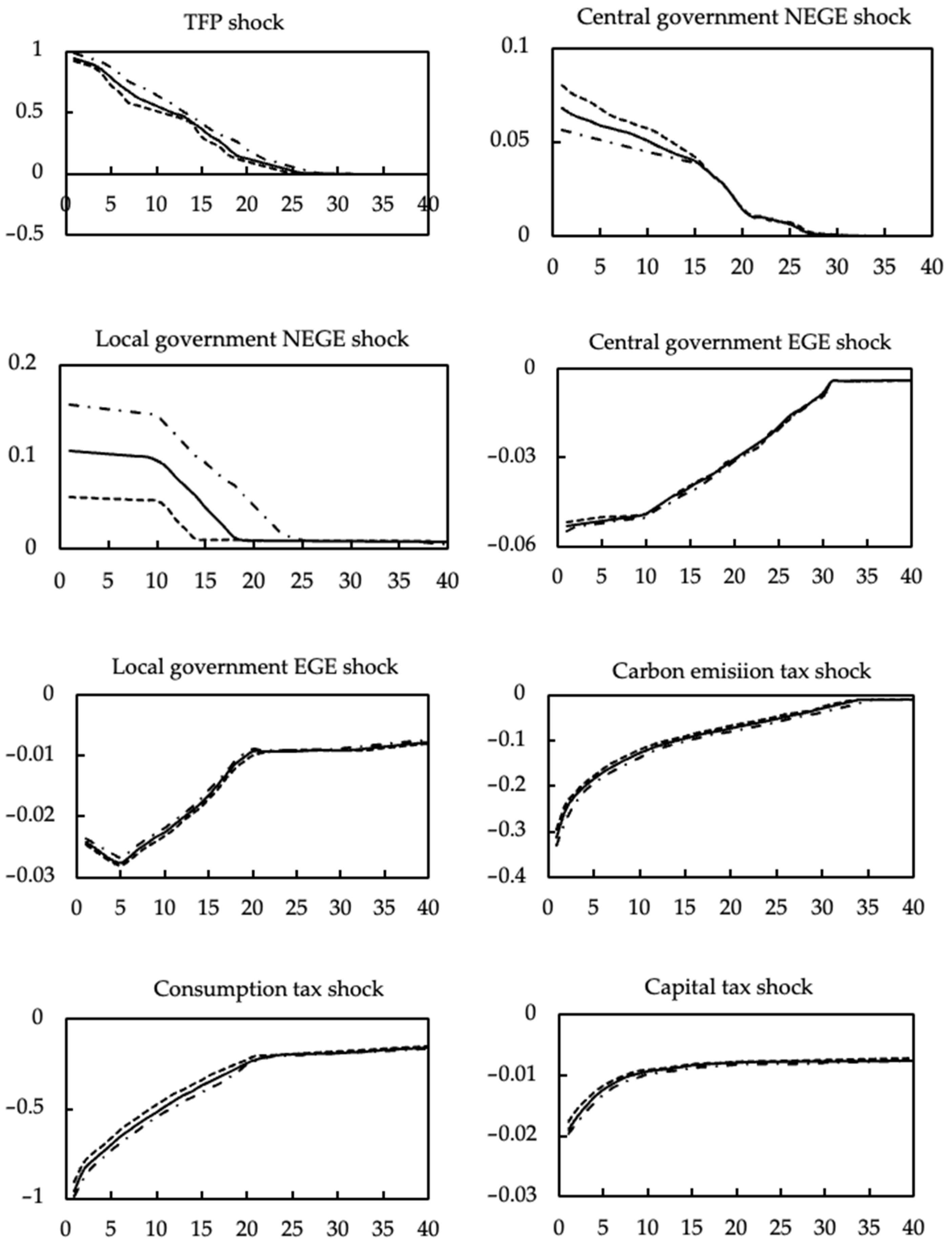
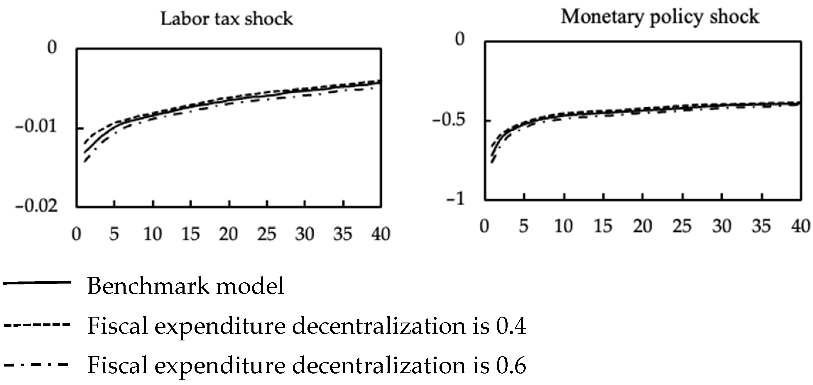
Figure 1 portrays the impulse response of exogenous shocks and fiscal expenditure decentralization on output. It can be found that the positive technology shock reduces marginal cost, and if the firms expand the scale of production, the output will increase immediately. Since the marginal return of capital is positively correlated with NEGE, the increase in NEGE leads to an increase in the households’ investment demand, resulting in an aggregate demand effect, which in turn increases output. It is worth noting that the positive externality of local government NEGE to output is larger than the positive externality of central government NEGE in the short run. The increase in government EGE has improved the production environment and living environment, thus stimulating total output growth in the short run.

Similarly, the positive impact of local government EGE on output is larger than the positive impact of central government EGE in the short run. With a temporary increase in the carbon tax, firms face an increase in marginal costs and a decline in willingness to produce, resulting in a reduction in output. The consumption tax rate increases, the households’ consumption decreases, and the households prefer investment and leisure, causing the output to deviate downward from the steady state. The increase in the capital tax rate will reduce the households’, resulting in a lower return on capital, an increase in marginal cost, and a downward deviation of output from the steady state. An increase in the labor tax rate will reduce the households’ labor supply and cause the output to deviate downward from the steady state. Rising nominal interest rates make bank credit and capital investment less valuable, so total output falls.

For technology shock, local government NEGE shock, and local government EGE shock, the increase in fiscal expenditure decentralization strengthens the positive effect of these three shocks on the output. However, the increase in fiscal expenditure decentralization inhibits the positive effects of central government NEGE and EGE shocks on the output. The negative impact of carbon emission tax shock, consumption tax shock, capital tax shock, labor tax shock, and nominal interest rate shock on the output will further increase with fiscal expenditure decentralization.

5.1.2. The Impact of Fiscal Expenditure Decentralization on Environmental Pollution

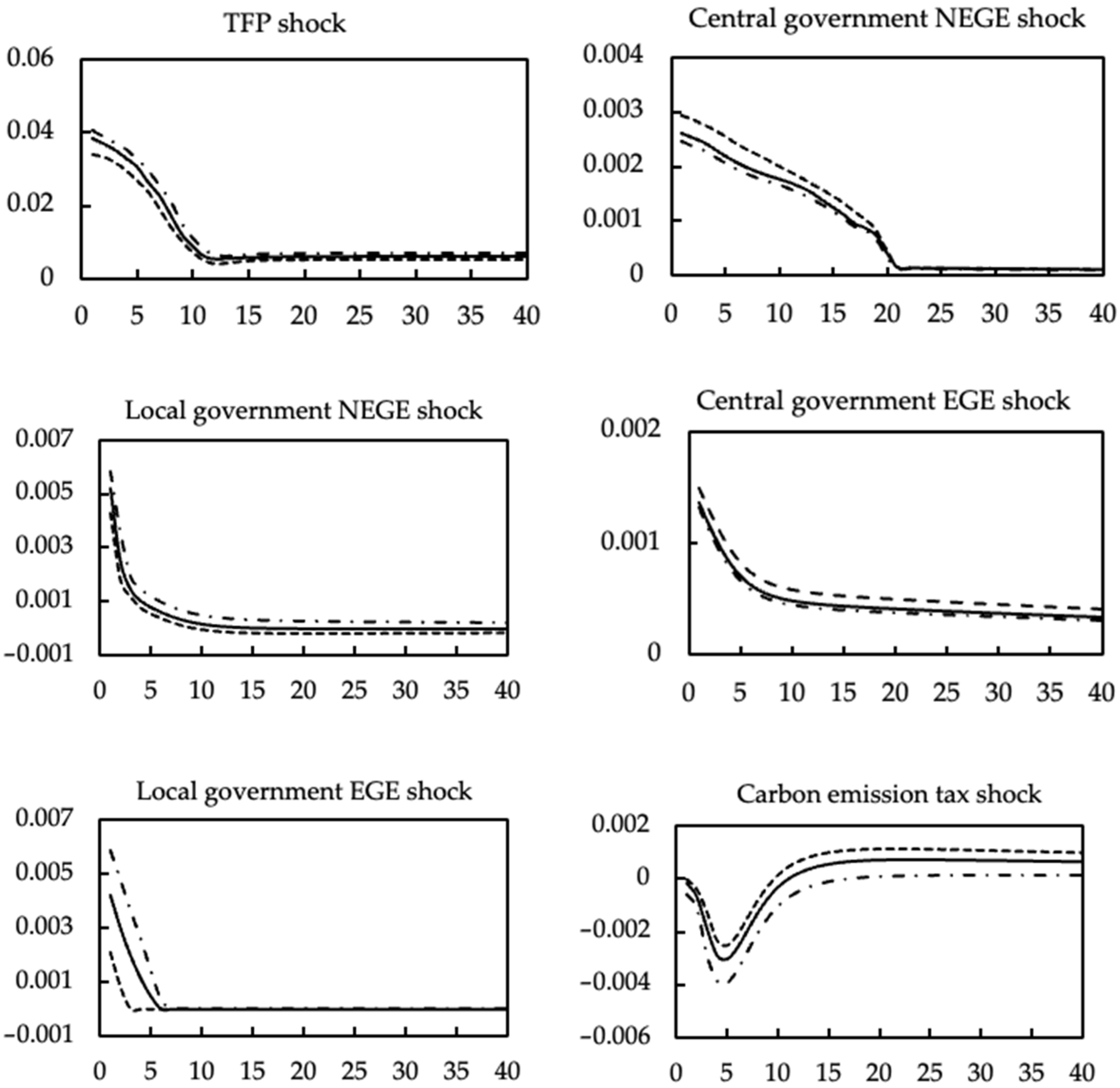
Figure 2 shows the impulse response of exogenous shocks and fiscal expenditure decentralization on environmental pollution. It is evident that technology shocks, government NEGE shocks, and government EGE shocks will cause environmental pollution, mainly due to increased carbon emissions due to the rise in output. The degree of environmental pollution caused by local government NEGE shock is greater than that of the central government NEGE shock. Carbon emission tax shocks, consumption tax shocks, capital tax shocks, labor tax shocks, and nominal interest rate shocks will improve environmental pollution, mainly because these five shocks will lead to a decline in output, and carbon emissions will also decrease with the decline in output.

For technology shock and local government NEGE shock, the increased fiscal expenditure decentralization further aggravates the environmental pollution. The impact of the central government NEGE shock will weaken the environmental pollution with increased fiscal expenditure decentralization. The impact of central government EGE shock, local government EGE shock, carbon emission tax shock, consumption tax shock, capital tax shock, labor tax shock, and nominal interest rate shock on the environmental pollution process will increase with the increase in fiscal expenditure decentralization.

5.2. Impulse Response Analysis of Fiscal Revenue Decentralization

5.2.1. The Impact of Fiscal Revenue Decentralization on Output

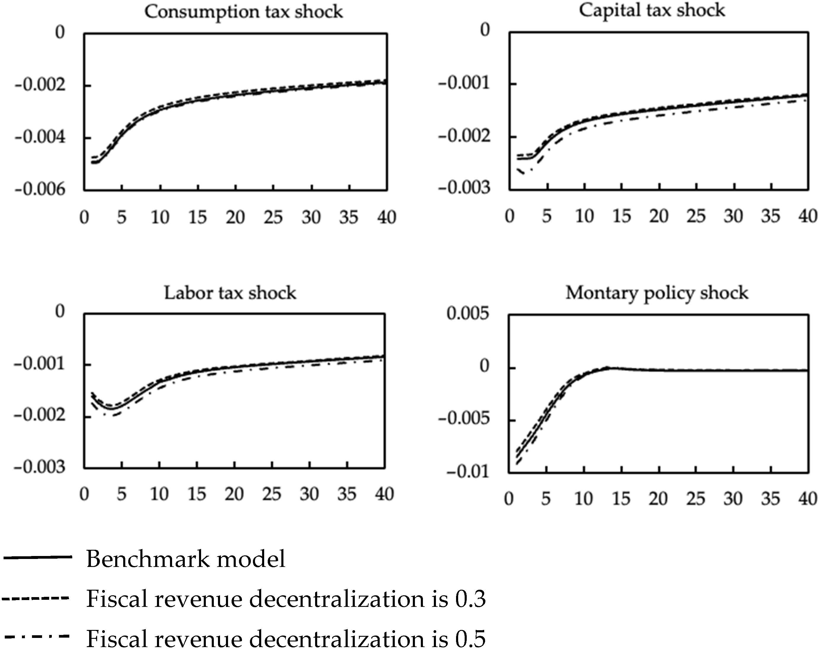
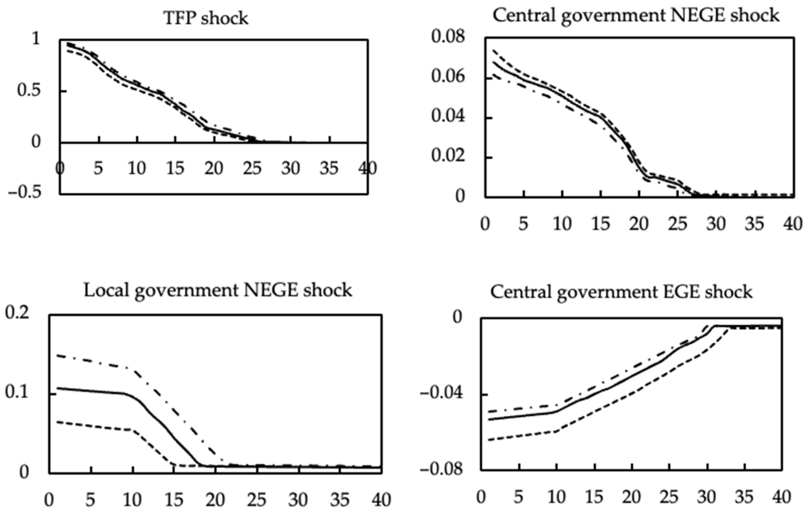
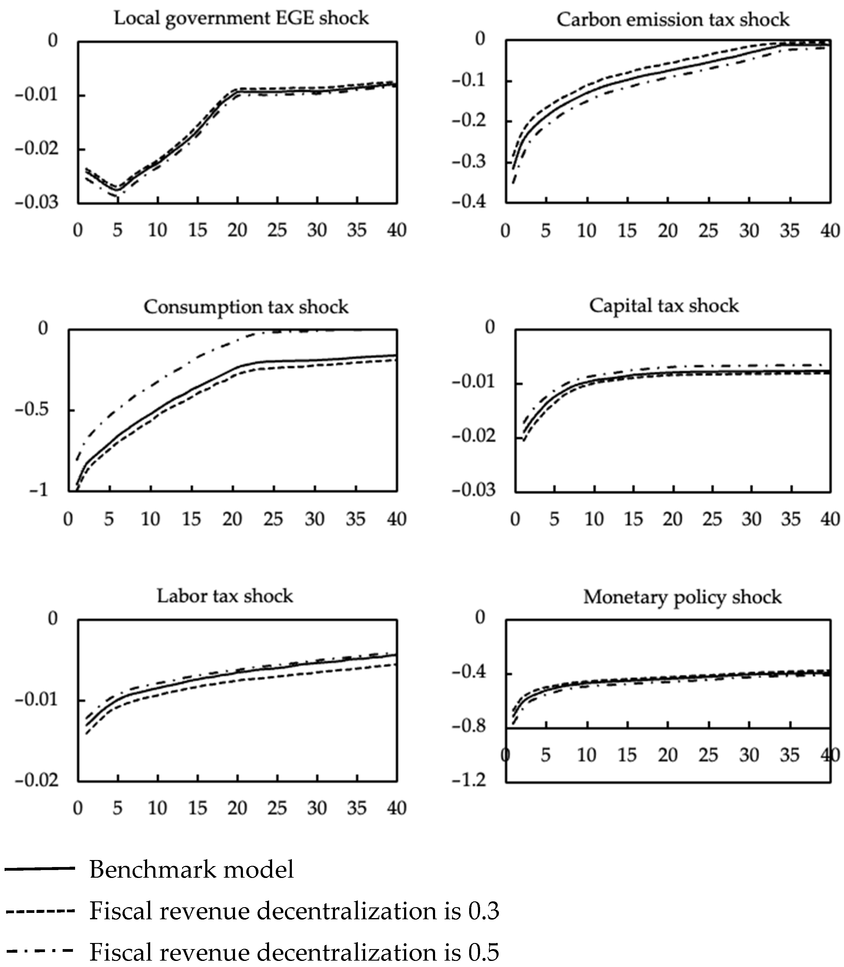
Figure 3 portrays the impulse response of exogenous shocks and fiscal revenue decentralization on output. For technology shock, local government NEGE shock, and local government EGE shock, the increase in decentralization of fiscal revenue strengthens the positive effect of these three shocks on output. However, the rise in the decentralization of fiscal revenue strongly inhibits the positive effect of the central government NEGE and the central government EGE on the output. The negative impact of carbon emission tax shock, consumption tax shock, capital tax shock, labor tax shock, and nominal interest rate shock on output will further increase with the increase in fiscal revenue decentralization.

5.2.2. The Impact of Fiscal Revenue Decentralization on Environmental Pollution

Figure 4 shows the impulse response of exogenous shocks and fiscal revenue decentralization on environmental pollution. It can be found that TFP shock and local government NEGE shock, the increase in fiscal revenue decentralization has further intensified the environmental pollution. With the increased fiscal revenue decentralization, the impact of the increase in central government NEGE on environmental pollution will be weakened. The effect of central government EGE shock, carbon emission tax, consumption tax, capital tax, labor tax, and nominal interest rate shock will further enhance the degree of environmental pollution with the increase in fiscal revenue decentralization.

5.3. Discussion

We measure the relative changes of social welfare on fiscal decentralization and local government behavior. Social welfare $W_t$ defines based on household’s utility function. Consumption compensation $\mathsf{\Phi }$ is the proportion of the consumption that needs to be compensated for the social welfare of changes in fiscal decentralization and local government behavior to be equal to the social welfare of the benchmark model $W_t^{\ast }$. The specific definitions are as follows.

$$W_t^{\ast }=E_t{\displaystyle \sum _{t=0}^{\propto }{\beta }^t}\left(\ln C_t-{\mu }_N\frac{N_t^{1+\eta }}{1+\eta }-\ln M_t\right)$$

(15)

$$W_t^{\ast }=E_t{\displaystyle \sum _{t=0}^{\propto }{\beta }^t}\left[\ln \left(1+\mathsf{\Phi }\right)C_t-{\mu }_N\frac{N_t^{1+\eta }}{1+\eta }-\ln M_t\right]$$

(16)

The results of the welfare analysis are shown in

Table 3. Calculation results of welfare analysis.

Model	Degree of Decentralization	Local Government Behavior	Social Welfare	Environmental Pollution	Consumption Compensation
Benchmark model	${\theta }_1=0.5,{\theta }_2=0.5$	0.01	−3.3920	17.7264	0.0997
		0.03	3.2960	17.7027	0
		0.05	−3.2663	17.6842	−0.0301
Fiscal expenditure decentralization	${\theta }_1=0.4,{\theta }_2=0.4$	0.01	−3.3372	17.7320	0.0411
		0.03	−3.1926	17.7171	−0.0991
		0.05	−3.2770	17.7063	−0.0198
Fiscal expenditure decentralization	${\theta }_1=0.6,{\theta }_2=0.6$	0.01	−4.4685	17.7198	0.1871
		0.03	−3.2190	17.6834	0.0749
		0.05	−3.2762	17.6527	−0.0205

. First, deepening fiscal expenditure decentralization is conducive to improving social welfare and alleviating environmental pollution. Second, the local government fiscal expenditure is biased on EGE, which is conducive to improve social welfare and reduce the environmental pollution.

6. Conclusions

This paper presents a E-DSGE model of multi-level governments and studies the impact of fiscal decentralization on the environmental policy in China. Our main results can be summarized as follows.

First, the imposition of a carbon tax will increase firms’ marginal cost and reduce their willingness to produce, resulting in a decline in output. However, the imposition of a carbon tax is beneficial to improving environmental pollution, mainly because the imposition of a carbon tax will lead to a decrease in output. Thus, the amount of carbon emissions will also decrease with the decline in output.

Second, deepening fiscal decentralization has heterogeneous effects on central and local fiscal expenditures. Deepening fiscal decentralization strengthens the positive externality of local government expenditures to output, but it also leads to further deterioration of environmental pollution. The positive externality of the central government expenditure will weaken with the increase in fiscal decentralization, but it is conducive to improving the quality of the environment.

Third, deepening fiscal decentralization is conducive to improving social welfare and alleviating environmental pollution. If the local government fiscal expenditures are biased on EGE, this is beneficial to improve social welfare and the quality of the environment.

Overall, we think the current fiscal decentralization system and the performance view based on GDP are the primary motivations for local governments to prefer NEGE to pursue regional economic growth. Although the effect of local government fiscal expenditure in stimulating economic growth is better than that of the central government, the environmental problem caused by the large amount of local government NEGE is also worthy of our attention.

We argue that it is necessary to clarify further the scope of financial and administrative powers of the central and local governments. It is crucial to change the GDP-based view of political performance and appropriately increase the proportion of livelihood indicators such as environmental governance and ecological protection in the evaluation system for official promotion.

The main contribution of this paper is that we incorporate the central and local government structure into a standard E-DSGE model, where the local governments implement fiscal policies through the trade-off between pursuing economic growth and environmental governance. However, this paper still has some limitations, which need to be further studied in the future. First, local government behavior is only limited to the bias of fiscal expenditures, but the connotation and extension of government behavior are very broad. Second, the local governments discussed in this paper are assumed to be homogeneous; that is, the local governments are the sum of all local governments in the real economy. However, the financial resources of local governments at all levels in the real economy are quite different, so there is a lack of further heterogeneity analysis. Third, this paper concludes that deepening fiscal decentralization is beneficial to the improvement of environmental quality and social welfare, but the optimal degree of fiscal decentralization has not been deeply discussed.

References

- Liu, J.; Bai, J.; Deng, Y.; Chen, X.; Liu, X. Impact of energy structure on carbon emission and economy of China in the scenario of carbon taxation. Sci. Total Environ. 2020, 762, 143093. [Google Scholar] [CrossRef]
- Zhang, J. Impacts of the emissions policies on tourism: An important but neglected aspect of sustainable tourism. J. Hosp. Tour. Manag. 2021, 47, 453–461. [Google Scholar] [CrossRef]
- Cao, J.; Dai, H.; Li, S.; Guo, C.; Ho, M.; Cai, W.; He, J.; Huang, H.; Li, J.; Liu, Y.; et al. The general equilibrium impacts of carbon tax policy in China: A multi-model comparison. Energy Econ. 2021, 99, 105284. [Google Scholar] [CrossRef]
- Glazer, A. Local regulation may be excessively stringent. Reg. Sci. Urban Econ. 1999, 29, 553–558. [Google Scholar] [CrossRef]
- Levinson, A. Environmental Regulatory Competition: A Status Report and Some New Evidence. Natl. Tax J. 2003, 56, 91–106. [Google Scholar] [CrossRef]
- Tiebou, C.M. A Pure Theory of Local Expenditure. J. Political Econ. 1956, 64, 416–424. [Google Scholar] [CrossRef]
- Stigler, G.J. Perfect Competition, Historically Contemplated. J. Political Econ. 1957, 65, 1–17. [Google Scholar] [CrossRef]
- Hayek, F.A. The Use of Knowledge in Society. Am. Econ. Rev. 1945, 35, 519–530. [Google Scholar] [CrossRef][Green Version]
- Silva, E.C.; Caplan, A.J. Transboundary Pollution Control in Federal Systems. J. Environ. Econ. Manag. 1997, 34, 173–186. [Google Scholar] [CrossRef]
- Khan, Z.; Ali, S.; Dong, K.; Li, R.Y.M. How does fiscal decentralization affect CO2 emissions? The roles of institutions and human capital. Energy Econ. 2020, 94, 105060. [Google Scholar] [CrossRef]
- Chen, G.; Xu, J.; Qi, Y. Environmental (de)centralization and local environmental governance: Evidence from a natural experiment in China. China Econ. Rev. 2022, 72, 101755. [Google Scholar] [CrossRef]
- Lingyan, M.; Zhao, Z.; Malik, H.A.; Razzaq, A.; An, H.; Hassan, M. Asymmetric impact of fiscal decentralization and environmental innovation on carbon emissions: Evidence from highly decentralized countries. Energy Environ. 2021, 33, 752–782. [Google Scholar] [CrossRef]
- Fredriksson, P.G.; List, J.A.; Millimet, D.L. Bureaucratic corruption, environmental policy and inbound US FDI: Theory and evidence. J. Public Econ. 2003, 87, 1407–1430. [Google Scholar] [CrossRef]
- Oates, W.E.; Portney, P.R. The Political Economy of Environmental Policy. Handbook Environ. Econ. 2003, 1, 325–354. [Google Scholar] [CrossRef]
- Kunce, M.; Shogren, J.F. Destructive Interjurisdictional competition: Firm, Capital and Labor Mobility in a Model of Direct Emission Control. Ecol. Econ. 2007, 60, 543–549. [Google Scholar] [CrossRef]
- Konisky, D.M. Regulatory Competition and Environmental Enforcement: Is There a Race to the Bottom? Am. J. Political Sci. 2010, 51, 853–872. [Google Scholar] [CrossRef]
- Sigman, H. Decentralization and Environmental Quality: An International Analysis of Water Pollution Levels and Variation. Land Econ. 2014, 90, 114–130. [Google Scholar] [CrossRef]
- Zeng, S.; Gao, L.; Shen, R.; Ma, Y.; Li, H. Fiscal Decentralization, Pollution and China’s Tourism Revenue. Sustainability 2020, 12, 1925. [Google Scholar] [CrossRef]
- Xia, S.; You, D.; Tang, Z.; Yang, B. Analysis of the Spatial Effect of Fiscal Decentralization and Environmental Decentralization on Carbon Emissions under the Pressure of Officials’ Promotion. Energies 2021, 14, 1878. [Google Scholar] [CrossRef]
- Heutel, G. How should environmental policy respond to business cycles? Optimal policy under persistent productivity shocks. Rev. Econ. Dyn. 2012, 15, 244–264. [Google Scholar] [CrossRef]
- Annicchiarico, B.; Dio, F.D. Environmental policy and macroeconomic dynamics in a new Keynesian model. J. Environ. Econ. Manag. 2015, 69, 1–21. [Google Scholar] [CrossRef]
- Hao, Y.; Chen, Y.; Liao, F.H.; Wei, Y.M. China’s fiscal decentralization and environmental quality: Theory and an empirical study. Environ. Dev. Econ. 2020, 25, 159–181. [Google Scholar] [CrossRef]
- Ying, T.C. Are macroeconomic policies better in curbing air pollution than environmental policies? A DSGE approach with carbon-dependent fiscal and monetary policies. Energy Policy 2020, 141, 111454. [Google Scholar] [CrossRef]
- Christiano, L.; Eichenbaum, M.; Rebelo, S. When is the government spending multiplier large? J. Political Econ. 2011, 119, 78–121. [Google Scholar] [CrossRef]
- Barro, R. Government spending in a simple model of endogenous growth. J. Political Econ. 1990, 98, 103–125. [Google Scholar] [CrossRef]
- Annicchiarico, B.; Dio, F.D. GHG Emissions Control and Monetary Policy. Environ. Res. Econ. 2017, 67, 1–29. [Google Scholar] [CrossRef]
- Rotemberg, J. Sticky Prices in the United States. J. Political Econ. 1982, 90, 1187–1211. [Google Scholar] [CrossRef]
- Galí, J. Monetary Policy, Inflflation, and the Business Cycle: An Introduction to the New Keynesian Framework; Princeton University Press: Princeton, NJ, USA, 2009. [Google Scholar]
- Xiao, B.; Fan, Y.; Guo, X. Dynamic interactive effect and co-design of SO2 emission tax and CO2 emission trading scheme. Energy Policy 2021, 152, 112212. [Google Scholar] [CrossRef]
- Angelopoulos, K.; Economides, G.; Philippopoulos, A. First-and second-best allocations under economic and environmental uncertainty. Int. Tax Public Finan. 2013, 20, 360–380. [Google Scholar] [CrossRef]
- Annicchiarico, B.; Diluiso, F. International transmission of the business cycle and environmental policy. Res. Energy Econ. 2019, 58, 101112. [Google Scholar] [CrossRef]
- Nordhaus, W.D. Projections and uncertainties about climate change in an era of minimal climate policies. Am. Econ. J. Econ. Policy 2017, 10, 333–360. [Google Scholar] [CrossRef]
- Smets, F.; Wouters, R. An Estimated Stochastic Dynamic General Equilibrium Model of the Euro Area. J. Eur. Econ. Assoc. 2003, 1, 1123–1175. [Google Scholar] [CrossRef]