Abstract
High-quality data are always desirable for superior decision-making in smart buildings. However, latency issues, communication failures, meter glitches, etc., create data anomalies. Especially, the redundant/duplicate records captured at the same time instants are critical anomalies. Two such cases are the same timestamps with the same energy consumption reading and the same timestamps with different energy consumption readings. This causes data inconsistency that deludes decision-making and analytics. Thus, such anomalies must be properly identified. So, this paper performs an enumeration of redundant data anomalies in smart building energy consumption readings using an analytical approach with 4-phases (sub-dataset extraction, quantification, visualization, and analysis). This provides the count, distribution, type, and correlation of redundancies. Smart buildings’ energy consumption dataset of Darmstadt city, Germany, was used in this study. From this study, the highest count of redundancies is observed as 5060 on 26 January 2012 with the average count of redundancies at the hour level being 211 and the minute level being 7. Similarly, the lowest count of redundancies is observed as 89 on 24 January 2012. Further, out of these 5060 redundancies, 1453 redundancies are found with the same readings and 3607 redundancies are found with different readings. Additionally, it is identified that there are only 14 min out of 1440 min on 26 January 2012 without having any redundancy. This means that almost 99% of the minutes in the day possess some kind of redundancies, where the energy consumption readings were recorded mostly with two occurrences, moderately with three occurrences, and very few with four and five occurrences. Thus, these findings help in enhancing the quality of data for better analytics.
1. Introduction
Smart grid evolution is ramping up in the present global energy scenario by offering deregulated markets, prosumer enablement, and unmatched comforts to electricity users [1]. Further, the advanced developments in information and communication technologies embedded smartness in the power grids. This smart technology enables people to manage their energy consumption by sending timely notifications. Moreover, it helps the utilities to understand the energy needs and consumption behaviors of the people. In view of all these benefits, in recent years, people are showing greater interest in making their buildings smarter to enhance energy utilization and comforts, thereby; the smart buildings’ culture is growing day by day globally. A smart building network is equipped with several types of sensors, which continuously sense the data from active appliances [2]. In the case of energy metering infrastructure, recording the consumption, transmitting the readings, processing and analysis, and decision-making plays a vital role. Further, from a smart grid perspective, there are many functionalities such as demand response, load management, event/outage management, contingency forecasting, etc., have to be provided. These functionalities help to manage the grid effectively by taking informed decisions timely. However, for all these, the availability of high-quality metered data for smart buildings is always desired to realize superior functionality [3,4,5].
However, the collection of high-quality data is always a challenge, which influences the effectiveness of all the above-mentioned operations. The quality of the data is usually tampered with due to the latency issues and malfunctioning of metering devices, communication and networking devices, processor-control units, energy thefts, cyber-attacks, etc., which creates anomalies in data collection. So, the analysis of such an accumulated database is highly important to better use the data for effective system operations [6]. Additionally, the data collected from multiple sources may have different characteristics in large volumes. Hence, it is very difficult to describe the quality of data even if it is collected in a well-defined manner [7]. Thus, a thorough understanding of such databases requires a systematic analysis of anomalies to deliver quality decisions [8].
The anomaly can be any deviation or abnormality in the usual expectation, such as redundant readings, missing readings, stray readings (outliers), incorrect readings, anonymous readings (garbage values), etc., that is observed in the captured database [9,10]. These anomalies lead to unreliable/inconsistent data collection, which deludes the billing and decision-making (e.g., demand response, customer segmentation, load management, etc.). Among all these data anomalies, redundant data is one of the high-impact issues that are observed in smart meter data. Generally, a record is said to be redundant if the entire data are the same as with the previous record(s). However, here the case is different for the energy consumption readings dataset. A record of the energy consumption dataset consists of timestamp information and its corresponding energy consumption reading. There are two possible issues that usually occur with respect to these records, viz., (i) the existence of redundant (duplicate) timestamps with the same readings, and (ii) the existence of redundant timestamps with different readings. Hence, it is crucial to analyze the redundant anomaly issue for executing accurate analytics to achieve optimal system operation and energy usage, which is the major focus of this paper. In this line, various state-of-the-art literature works representing the significance of data quality issues in the power systems domain are detailed as follows.
The data quality issues that exist in smart grid environments were discussed in terms of noise, incompleteness, and outliers. The methods for finding causes of outliers in the electrical consumption data were discussed in [11]. Similarly, a systematic review of smart meter data analytics was performed with descriptive, predictive, and prescriptive analytics on applications such as abnormality detection, load forecasting, and customer categorization, etc., [12,13]. Further, an analysis was performed for detecting the bad data in the distribution systems [14]. Usually, smart meters or multi-function meters trace the information of electrical voltages. To detect the short-duration abnormalities in these voltages an algorithm was developed in [15]. To detect bad data from the collected phasor measurement units’ data, a data-driven algorithm was proposed based on spectral clustering [16]. Further, to minimize the data losses in smart grids, a technique named “compressive sensing” was presented in [17]. A graph comparison-based approach was proposed in [18] for detecting the anomaly (deviation in the voltage values from the specified or threshold value) in the database of the electrical network.
From the above discussion, even though there were some research works related to smart grid data quality, no research work has focused on redundant data anomalies, to the best of the authors’ knowledge. However, there were some works regarding duplicate data analysis in some other applications as described follows.
Several similarity metrics such as character-based, token-based, phonetic-based, and numeric-based were discussed in [19] for duplicate record identification using various supervised, semi-supervised, and unsupervised learning techniques. However, all these metrics are useful to identify duplicates in textual documents. A new method named ‘XMLDup’ was proposed in [20] to identify duplicates in XML data. This was implemented by a Bayesian network. Usually, the duplicates in large volumes of data identified within a short duration would be useful. So, several progressive methods were proposed to do this task [21]. To process complex queries on the unmerged duplicates in the probabilistic databases, an entity-join operator was proposed in [22]. A system named ‘SiLo’ was proposed for data deduplication. This system was implemented with a similarity and locality-based indexing mechanism [23]. Further, an application named ‘AppDedupe’ was proposed for data deduplication in the cloud environment. This application performs data deduplication by generating application-aware similarity indices [24].
A domain-independent framework named ‘DaPo’ was proposed to detect duplicates in large datasets. This framework was created using Apache Spark [25]. Similarly, three constraint-based techniques were proposed in [26] to reduce the duplication of substructures in graph mining and to further improve the cost of mining. The comprehensive frameworks such as single and multiple strategies were applied to the database for normalizing the duplicate records at various granularities [27]. Further, a three-step approach was proposed to detect duplicate records in incomplete and noisy data. The first step was initially focused on similarity score finding, the second step was representing records uniquely by grouping them, and the final step was the refinement of groups [28]. The concept of preprocessing was discussed in predictive data mining to maintain the reliability of the dataset [29]. The data deduplication technique for removing redundant data was discussed and also compared data deduplication with data compression in [30]. Further, the review of data reduction methods presented in [31] revealed that no method alone would perform the desired data reduction on all 6V’s of big data. It was also provided with the information that the data reduction was importantly based on volume and variety. To do this, various architectures were discussed in [32] for delivering proficient functions related to data management towards the effective processing of big data.
In summary, the abovementioned literature mainly shows works related to duplicate identification in textual information, bad data detection, and deduplication of data when such anomalies exist. However, these approaches are not sufficient for redundant data anomaly analysis with respect to smart building energy datasets due to the presence of two types of redundancy anomaly characteristics as described above. Hence, to address the issue of detecting redundant data anomalies, this paper implements an analytical enumeration for smart buildings’ energy consumption datasets. It involves a 4-phase approach (phase-1: sub-dataset extraction, phase-2: quantification, phase-3: visualization, and phase-4: analysis). Where, phase-1 prepares the original smart buildings’ energy consumption dataset into a required format. It extracts the redundant records with the same timestamps and represents them as a sub-dataset that is used for further analysis in phase-2 to phase-4. Phase-2 quantifies the redundancies at the day/hour/min level and finds minutes with no redundancies. Phase-3 visualizes the hourly distribution of redundancies and min/sec-wise occurrence of readings. Phase-4 analyzes the types of redundancies and their correlation at the hour/min level. As a whole, this enumeration provides count, distribution, type, and correlation of the redundancies. The search process continues till the end of the records and detects all types of redundant data anomalies present in the energy consumption dataset, which is the major contribution of this paper.
The rest of the paper is structured as follows. Section 2 presents the description of the considered real-time case study to implement the proposed analytical enumeration. Section 3 presents the logical flow and detailed implementation of the analytical enumeration. Section 4 presents the comprehensive simulation results and their inferences. Finally, Section 5 concludes the findings of the paper in a consolidated and constructive way with the observations made over various phases.
2. Tracebase Dataset Case Study: From Darmstadt, a Smart City in Germany
The tracebase dataset that is available at [33] is one of the standard and widely used public datasets that consists of energy consumption readings of smart buildings. This dataset was captured during 2011–2013 and thoroughly explored [34,35,36,37]. It consists of energy consumption readings of 43 appliances and 158 devices in the smart buildings of the cities of Darmstadt, Germany, and Sydney, Australia. So, it is a huge and useful dataset when compared with other datasets [36], which may consist of more hidden issues that help the energy consumption-related research studies.
In this view, it is observed that many researchers have considered this dataset for conducting various analyses on energy consumption data such as non-intrusive load monitoring and anomalous behavior [3,4,5,38,39,40,41], energy consumption behavior and forecasting [42,43,44], energy disaggregation and load shedding [45,46,47], appliance identification [48], etc. However, from this literature review, it is observed that no such analysis exists to detect various data quality issues related to redundancy, which is the key point of focus in this paper.
Thus, this paper uses the energy consumption readings dataset collected from Darmstadt city for the analysis, which is a part of the tracebase dataset. This dataset consists of three directories, viz., ‘complete’, ‘incomplete’, and ‘synthetic’. Among these three, the ‘complete’ directory is considered for the execution of the proposed analytical enumeration as it consists of all readings of appliances. This directory includes several subdirectories that represent various appliances used in smart buildings. Each subdirectory comprises a list of “comma-separated values (CSV)” files representing the number of days on which the appliance was connected. These files are named with a combination of the appliance identifier and the date on which it is connected. The records in the CSV files are called traces that represent the timestamps and corresponding energy consumption readings. These traces are collected as one trace for each second. The collection of these traces usually starts at midnight and ends at next-day midnight. The information of traces is stored on a 24-h clock. The format of the trace is “Day/Month/Year Hour:Minute:Second; Reading1; Reading2 (e.g., 26/01/2012 06:32:58;34;62)”. The readings represent active power measurements of appliances connected to the advanced metering infrastructure [49]. As these two readings are of the same nature, only Reading1 is considered in this paper for the enumeration. Throughout this paper, the word “file” indicates the information of a day given in terms of a table and the word “record” indicates a row in the given file.
The redundancy count is observed for all the appliances in January 2012 and is plotted as shown in Figure 1, as it is observed that, January 2012 is having the connectivity of more appliances compared to other months recorded in the dataset.
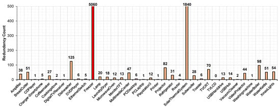
Figure 1.
Redundancy count of different appliances.
From this plot, it is observed that the freezer appliance has the highest redundancy count of 5060 when compared to the other appliances, which is shown with a red colored bar. Hence, this appliance is considered in this paper for the enumeration as it can exhibit more information regarding redundancies because of having more redundancy count. The freezer dataset consists of CSV files corresponding to nine days (16 December 2011, 17 December 2011, and 20 January 2012 to 26 January 2012). All these are considered for enumerating the redundancies in this paper.
3. Description and Implementation of the Proposed Analytical Enumeration
The objective of the proposed study is to enumerate the total number of redundancies and their nature in smart building energy consumption data. The four phases of the proposed analytical enumeration, viz., sub-dataset extraction, quantification, visualization, and analysis are implemented as shown in the logical flow diagram given in Figure 2. This figure also shows various tasks that are assumed for each of these phases. All these tasks are achieved as per the implementation flow given in Figure 3. As described in Section 2, from the entire dataset, the freezer appliance data files are considered a precise case to implement the desired analytical enumeration. The entire study is implemented and simulated through “R programming (developed by Ross Ihaka and Robert Gentleman at the University of Auckland, New Zealand) and RStudio IDE (developed by RStudio, a public-benefit corporation in Massachusetts, United States, founded by J. J. Allaire)”. The following sections describe the detailed procedure of the implementation.
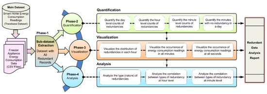
Figure 2.
Logical flow indicating various phases involved in the proposed analytical enumeration.
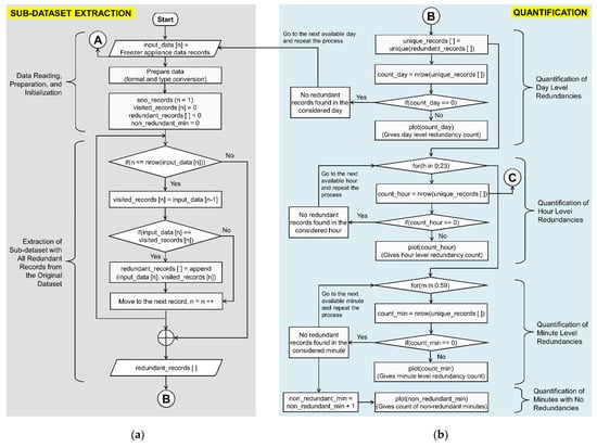
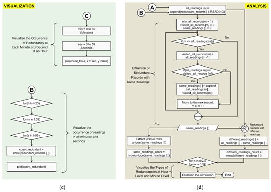
Figure 3.
Implementation of various phases involved in the proposed analytical enumeration. (a) Implementation of phase-1. (b) Implementation of phase-2. (c) Implementation of phase-3. (d) Implementation of phase-4.
3.1. Phase-1: Sub-Dataset Extraction
This phase extracts a properly prepared sub-dataset from the given complete freezer data that is required for the desired enumeration. As stated in Section 2, usually, the datasets that are captured from various smart meters have records in the form of “Day/Month/Year Hour:Minute:Second;Reading”, i.e., a combination of heterogeneous attributes. So, the direct usage of the original dataset makes the analysis complex, thus, it has to be prepared properly for the analysis. Further, to perform the enumeration of redundant data anomalies, the consideration of the entire original dataset for different visualizations and analyses may increase the computational complexity. So, this phase provides the filtered data in the form of a sub-dataset that is prepared as required and consists of the records that have duplicated/redundant timestamps (occurred more than once). The entire process involved in this phase is implemented in two steps as mentioned in Figure 3a which is described as follows. This reduced sub-dataset is directly used to perform the next phases.
3.1.1. Step-1: Data Reading, Preparation, and Initialization
The data of the smart building’s energy consumption are pre-processed in this step. To implement this, the freezer appliance data records are given as input for which the data preparation is done as follows. This appliance consists of CSV files available for nine days. Each CSV file represents a day individually. The freezer appliance data records are stored into “input_data [n]” with respect to the following rearrangement. All these records are originally available in a single column format, which cannot be directly used for the enumeration. Hence, it is required to split the single column into multiple columns by introducing new columns namely REC_DATE, REC_HOUR, REC_MINUTE, REC_SECOND, READING, where REC stands for RECORDED. Further, the data types of all these columns are to be changed as required. Additionally, the required variables for executing the analytical enumeration corresponding to phase-1 shown in Figure 3a are described and initialized as follows.
- “sno_records” represents the serial number of records “n” in the “input_data [n]”, which starts with 1 (i.e., initialized as n = 1).
- “visited_records [n]” represents an array of records that are already visited in “input_data [n]” during the search process. It is initialized to 0. Further, when the search progresses, the records in “visited_records [n]” increase.
- “redundant_records [ ]” represents an array of redundant timestamped records that are found during the search process. It is initialized to 0. It consists of only timestamps, but, no readings are included in this array.
- “non_redundant_min” represents the count of the minutes with no redundancy in “input_data [n]”. It is initialized to 0.
3.1.2. Step-2: Extraction of Sub-Dataset
Extraction of a sub-dataset with all the redundant timestamped records (without the READING column) from the original dataset (input_data [n]) is performed in this step. To implement this, the process starts with the first record, which is assigned to “visited_records [n]”. Now, the serial number of the record in “input_data [n]” is incremented. This current record of “input_data [n]” is compared with the current record of “visited_records [n]. If these two records are matched, they are appended and stored into “redundant_records [ ]”. This indicates the existence of redundant records with the same timestamps. If these records are not matched, then the process moves to the next record of the “input_data [n]” and it is stored in “visited_records [n]”.
This way, the comparison of “visited_records [n]” and “input_data [n]” is continued sequentially by incrementing “n” value (n = n++). This process continues till it reaches the end of the records by checking (n ≤ nrow(input_data [n])) in the dataset. Finally, a sub-dataset, “redundant_records [ ]” is extracted with all redundant records which have duplicated/redundant timestamps (occurred more than once). This sub-dataset is directly used to implement the next two phases, i.e., Quantification and Visualization. So, these two phases are applied to the timestamp information, but, not to the reading information. However, for phase-4, i.e., Analysis, the READING column is added to this sub-dataset. The reason for this consideration is mentioned as follows.
If the search process for redundant records is performed by considering both timestamps and readings, only the records with the same timestamps and the same readings will be fetched, and the records with the same timestamps and different readings will be omitted. However, both these varieties are considered redundant records. That is, the enumeration of redundancies will be incomplete as some of the records are ignored in the search process. To address this issue, the proposed enumeration initially performs enumerating redundancies with respect to timestamps and then redundancies with respect to readings.
3.2. Phase-2: Quantification
This phase provides the count of redundancies at the day level, hour level, and minute level. Further, it computes the total number of minutes with no redundancy that is available in the whole day considered. Initially, the count of redundancies occurring on all nine days is identified. This provides quantification of the day-level redundancies, using which, a day that contains a greater number of redundancies is identified. The day which has the highest count of redundancies is used for the quantification of redundancies at the hour level, using which; an hour that contains a greater number of redundancies is identified. Further, quantification of redundancies at the minute level is performed for that hour which exhibits the highest count of redundancies. Additionally, the overall count of minutes that are not exhibiting any redundancy is also quantified for the same day. The entire process involved in this phase is implemented as mentioned in Figure 3b and is described as follows.
- Quantification of day level redundancies: As mentioned in Section 3.1.1, the “redundant_records [ ]” consists of all the records that are occurring more than once. To quantify the exact count of redundancies in a day, it is required to count only the unique records (i.e., one out of the same records available). So, the process starts with separating the unique records from the “redundant_records [ ]” by using “unique(redundant_records [ ])” and storing them into “unique_records [ ]”. The count of all the records available in “unique_records [ ]” gives the number of redundancies that are available on that particular day. This is calculated using “nrow(unique_records [ ])” and stored into “count_day”. The same process is repeated for all days. İf, for any day, this count is equal to zero (i.e., count_day = = 0) indicating that there are no redundancies found that day, thereby, the process is moved to the next day. Further, the day-level redundancy count is plotted by using “plot(count_day)”.
- Quantification of hour level redundancies: For hour level quantification, the count of all the records available in each hour (for(h in 0:23)) is computed by using “nrow(unique_records [ ])” and stored into “count_hour”. İf, for an hour, this count is equal to zero (i.e., count_hour = = 0) indicating that there are no redundancies found in that hour, thereby, the process moved to the next hour. Further, the hour level redundancy count is plotted by using “plot(count_hour)”.
- Quantification of minute level redundancies: For minute level quantification, the count of all the records available in each minute (for(m in 0:59)) is computed by using “nrow(unique_records [ ])” and stored into “count_min”. If, for any minute, this count is equal to zero (i.e., count_min = = 0) indicates that there are no redundancies found in that minute, thereby, the process moved to the next minute. Further, the minute level redundancy count is plotted by using “plot(count_min)”.
- Quantification of minutes with no redundancies: The data capturing usually starts at midnight and ends the next day at midnight by following the 24-h clock as discussed in Section 2. There are 1440 min in 24-h. All these minutes may not contain redundancy. So, it is necessary to quantify the number of minutes out of total minutes that do not contain redundancy. This quantification provides an understanding of the level of redundancies occurring in a day. In the abovementioned process of minute level redundancies, if any minute is found having no redundancy count that information is counted as “non_redundant_min”. Further, it is sequentially incremented using “non_redundant_min = non_redundant_min + 1” when another minute with no redundancy is found. This process is verified for all the minutes in a day. Finally, the overall count indicated by “non_redundant_min” gives the count of the total number of non-redundant minutes in a day and is plotted by using “plot(non_redundant_min)”.
3.3. Phase-3: Visualization
This phase provides information on how the redundancies are distributed and occurred in each hour by suitable visualizations. This helps to easily understand and represent the level of redundancies that are present in a day/hour/minute. The detailed flow for the proposed visualization is given in Figure 3c and is described as follows.
- The required variables for executing the analytical enumerations that are given in phase-3 are described and initialized as,
- “min” represents the minutes that are to be considered for visualizing the occurrence of redundancy at each minute. It starts from 0 and varies up to 59 in an hour.
- “sec” represents the seconds that are to be considered for visualizing the occurrence of redundancy at each second. It starts from 0 and varies up to 59 in a minute.
- The actual occurrence of redundancies and their count in each hour (i.e., count_hour) are visualized by applying “plot(count_hour, x = sec, y = min)”.
- Further, the visualization is extended to all minutes and all seconds for a better understanding of the occurrence of energy consumption readings. The number of redundant records “nrow(redundant_records [ ])” is calculated by considering the extracted sub-dataset “redundant_records [ ]” and stored into “count_redundant”. This calculation is done at all minutes (for(m in 0:59)) and all seconds (for(s in 0:59)) of each hour (for(h in 0:23)), and are visualized by using “plot(count_redundant)”.
3.4. Phase-4: Analysis
The previous phases give the counts and distribution of redundancies in a day/hour/minute based on the timestamp information. Those phases use the sub-dataset (redundant_records [ ]) which only consists of the timestamps information as mentioned in Section 3.1.2. Along with this information, understanding the redundancy nature with respect to the readings is also important, which is the major focusing point of this phase. Hence, this phase provides information on types of redundancy in readings and their existence at the hour level and minute level. Additionally, it also provides the correlation between these types at the hour level and minute level. To achieve the desired analysis, it is required to have readings also along with their corresponding timestamps. For this purpose, the “redundant_records [ ]” have to be appended with readings (READING as mentioned in Section 3.1.1). Thus, a new object named “all_readings [m]” is prepared using “append(redundant_records [ ], READING)”. So, to carry out this proposed analysis of phase-4, the required variables as shown in Figure 3d are described and initialized as follows.
- “sno_all_records” represents the serial number of records “m” in the “all_readings [m]”, which starts with 1 (i.e., initialized as m = 1).
- “visited_all_records [m]” represents an array of records that are already visited in “all_readings [m]” during the search process. It is initialized to 0.
- “same_readings [ ]” represents an array of redundant records with the same timestamps and same readings. It is initialized to 0.
The entire analysis of this phase is carried out in three steps, namely, (i). Count of redundancy with the same timestamp and same readings (ii). Count of redundancy with the same timestamp and different readings, and (iii). Correlation analysis of (i) and (ii). These steps are explained as follows.
- Count of redundancy with the same timestamp and same readings: Extraction of the redundant records with the same readings from “all_readings [m]” is performed in this step. To implement this, the process starts with the first record, which is assigned to “visited_all_records [m]. Now, the serial number of the record in “all_readings [m]” is incremented. This current record in the “all_readings [m]” is compared with the current record of “visited_all_records [m]. If these two records are matched, they are appended and stored into “same_readings [ ]”. This indicates the existence of redundant records with the same readings. If these records are not matched, then the process moves to the next record of the “all_readings [m]” and is stored in “visited_all_records [m]”. This way, the comparison of “visited_all_records [m]” and “all_readings [m]” is continued sequentially by incrementing “m” value (m = m++). This process continues till it reaches the end of the records by checking (m ≤ nrow(all_readings [m])) in the dataset. Finally, the redundant records with the same readings, “same_readings [ ]” is extracted with all redundant records which have duplicated/redundant timestamps and readings. As these records occur more than once, it is necessary to select the unique records to identify the count of redundant records with the same readings from them by using “unique(same_readings [ ])”. From this, the count of these unique records is calculated by using “nrow(unique(same_readings [ ]))”. The information of this count is stored in “same_readings_count”.
- Count of redundancy with the same timestamp and different readings: Extraction of the redundant records with different readings is achieved by subtracting the “same_readings [ ]” from “all_readings [m]” and stored into “different_readings [ ]”. From this, the count of redundant records with different readings is calculated by using “nrow(different_readings [ ])”. The information of this count is stored in “different_readings_count”.
- Correlation analysis: To understand the parity of types of redundancies, a correlation analysis is performed between the count of redundant records with the same readings and the count of redundant records with different readings. This correlation is established by drawing a plot between “same_readings_count” and “different_readings_count” at each hour (for(h in 0:23)) and each minute (for(m in 0:59)).
4. Simulation Results and Discussion
To support the objective of this paper, the simulation results of the quantification phase are presented in Section 4.1, the visualization phase is presented in Section 4.2, and the analysis phase is presented in Section 4.3. Finally, Section 4.4 gives the validation of the proposed approach by comparing it with the machine learning-based conventional random forest approach. The outcomes of all these phases are explained as follows.
4.1. Results of Quantification Phase
This quantification phase is carried out to discuss four points, viz., quantification of redundancies at the day level (discussed in Section 4.1.1), quantification of redundancies at the hour level (discussed in Section 4.1.2), quantification of redundancies at the minute level (discussed in Section 4.1.3), and quantification of minutes with no redundancy for the day 26 January 2012 (discussed in Section 4.1.4) as explained follows.
4.1.1. Quantification of Redundancies at Day Level
The redundancies identified in the smart building energy consumption data at the day level are plotted as shown in Figure 4. This figure indicates the density of redundancies occurring at different instants in a day in the three-dimensional view (seconds on the x-axis, minutes on the y-axis, and hours on the z-axis). The subplots of Figure 4 represent the redundancy plots for all the days. These plots signify the high-level analysis of redundancies, which becomes a basis for the low-level analysis presented in subsequent sections. From these results, the count of redundancies is identified as follows.
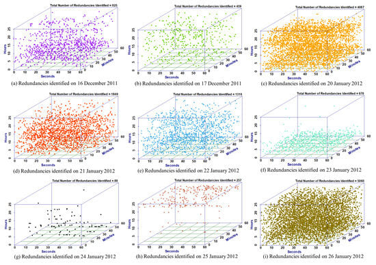
Figure 4.
Quantified redundancies at the day level for different days.
The redundancy count on 16 December 2011 is 925 as shown in Figure 4a, on 17 December 2011 is 459 as shown in Figure 4b, on 20 January 2012 is 4087 as shown in Figure 4c, on 21 January 2012 is 1849 as shown in Figure 4d, on 22 January 2012 is 1316 as shown in Figure 4e, on 23 January 2012 is 678 as shown in Figure 4f, on 24 January 2012 is 89 as shown in Figure 4g, on 25 January 2012 is 257 as shown in Figure 4h, on 26 January 2012 is 5060 as shown in Figure 4i. From these plots, it is observed that the count of redundancies is high (5060) on 26 January 2012, which is considered the worst case and is low (89) on 24 January 2012 which is considered as best case. Hence, the day 26 January 2012 is considered for further analysis which can give a better perspective on redundancies.
4.1.2. Quantification of Redundancies at Hour Level
This section gives the count of redundancies identified at the hour level of a day as shown in Figure 5. For this hour-level analysis, the day (i.e., 26 January 2012) which has the highest redundancy count (5060) as discussed in Section 4.1.1 is considered. So, on this particular day, the redundancy counts for all the hours (24 h are represented from 0 to 23) are quantified. The obtained hour level redundancy counts are arranged in descending order with respect to corresponding hours as shown in Figure 5. From this, the maximum and minimum redundancy counts are observed as, 431 at Hour 3 and 162 at Hours 17 and 23, respectively, with an average redundancy count per hour is 211.
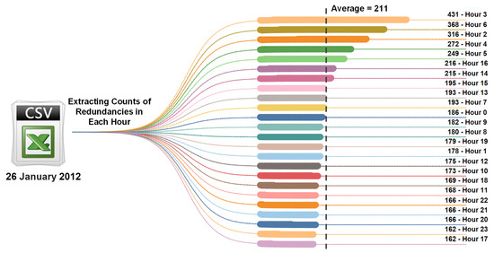
Figure 5.
Quantified redundancies at the hour level in descending order.
4.1.3. Quantification of Redundancies at Minute Level
This section gives the count of redundancies identified at the minute level of an hour as shown in Figure 6. For this minute-level analysis, Hour 3, which has the highest redundancy count (431) as discussed in Section 4.1.2, is considered. So, in this particular hour, the redundancy counts for all the minutes (from 0 to 59) are quantified. From this, the maximum and minimum redundancy counts are observed as, 13 (which is shown with a red colored bar) at minute 16 and 2 at minutes 48 and 54, respectively, with an average redundancy count per minute is 7.
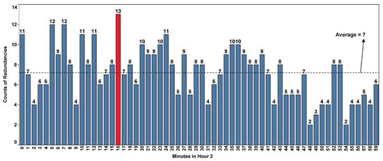
Figure 6.
Quantified redundancies at minute level in hour 3.
4.1.4. Quantification of Minutes with No Redundancy
The redundancy counts of all the 1440 min (whole day) of 26 January 2012 are plotted hour-wise as shown in Figure 7 to find the availability of minutes with no redundancy. For a better view, four hours are considered for each subplot as shown in Figure 7a–f. The bars in these subplots represent the redundancy count in that corresponding minute. So, if no bar is generated at a minute indicates zero redundancies in it. All such minutes are pointed out with a red arrow mark for clear identification. From these plots, it is observed that Minute 32 of Hour 1 (Figure 7a), Minute 50 of Hour 5 and Minute 31 of Hour 7 (Figure 7b), minutes 5 and 17 of Hour 8 (Figure 7c), Minute 7 of Hour 12, Minute 0 of Hour 13, and Minute 23 of Hour 15 (Figure 7d), Minute 20 of Hour 18 and Minute 58 of Hour 19 (Figure 7e), minutes 21, 41, and 52 of Hour 22, and Minute 32 of Hour 23 (Figure 7f) do not contain the redundancy. So, from this quantification, it is found that only14 out of 1440 min do not have redundancies. This adds weight to the importance of redundancy analysis for smart buildings’ energy consumption data which have to be carefully visualized and addressed to better improve analytics. So, further in-depth visualization and analysis are given in the sections below.
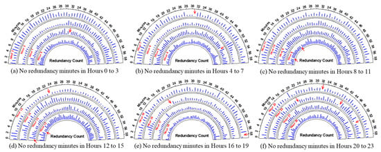
Figure 7.
Depiction of the minutes with no redundancy identified on 26 January 2012.
4.2. Results of Visualization Phase
This visualization is carried out in three steps. The results of redundant data that occurred in each hour are given in Section 4.2.1 and the occurrence of energy consumption readings in minutes/seconds-wise is given in Section 4.2.2 and Section 4.2.3, respectively.
4.2.1. Visualizing the Distribution of Redundancies in Each Hour
The visualization of hour-level redundancy distribution is carried out for all hours of the day 26 January 2012. For this, some of the hours (2, 3, 6, 11, 18, and 23) of the day are considered and plotted as shown in Figure 8. These hours are selected based on their peculiarity in redundancy occurrences when compared to other hours. This visualization gives the mapping of redundancy occurrences with respect to the minutes and seconds of a considered hour, i.e., exact instant information where the redundancy occurs. For this purpose, the seconds’ information is plotted on the x-axis and the minutes’ information is plotted on the y-axis. Along with the distribution of redundancies in an hour, the count of redundancies also can be observed from these plots. The counts identified are 316 in Hour 2 (Figure 8a), 431 in Hour 3 (Figure 8b), 368 in Hour 6 (Figure 8c), 168 in Hour 11 (Figure 8d), 169 in Hour 18 (Figure 8e), 162 in Hour 23 (Figure 8f).
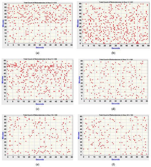
Figure 8.
Illustration of the distribution of redundancies in each hour. (a) Redundancies occurring at Hour 2. (b) Redundancies occurring at Hour 3. (c) Redundancies occurring at Hour 6. (d) Redundancies occurring at Hour 11. (e) Redundancies occurring at Hour 18. (f) Redundancies occurring at Hour 23.
4.2.2. Visualizing the Occurrence of Energy Consumption Reading in All Minutes
To understand the existence of redundancies with respect to all minutes of an hour, the minute-wise occurrence of energy consumption readings in Hour 22 is plotted as shown in Figure 9. This analysis is performed at all hours of the day 26 January 2012.
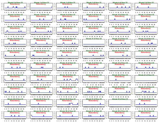
Figure 9.
Depiction of the occurrence of energy consumption readings in all minutes of Hour 22.
However, the case of Hour 22 is shown in this section as this hour has a mix of minutes with no redundancy and redundancies, which gives a better understanding compared to other hours. In Figure 9, the seconds of a minute in the considered hour are taken on the x-axis and the number of occurrences of an energy consumption reading is taken on the y-axis. In this plot, if the occurrence of energy consumption reading is greater than ‘1’, then it indicates a redundant reading at that particular second of the minute. Therefore, from Figure 9, it can be observed that, except for minutes 21, 41, and 52, the plots of all the other minutes possess some fluctuation. Hence, 57 min out of 60 min of Hour 22 are having redundant readings.
4.2.3. Visualizing the Occurrence of Energy Consumption Reading in All Seconds
The occurrence of energy consumption readings at all seconds of some particular minutes is plotted as shown in Figure 10. This visualization is carried out on all minutes of all hours. To show all the possibilities, the plots of Minute 32 of Hour 23, Minute 9 of Hour 2, Minute 36 of Hour 3, Minute 50 of Hour 6, Minute 19 of Hour 11, and Minute 5 of Hour 18 are given. Here in this figure, green colored bar indicates 1 occurrence, orange colored bar indicates 2 occurrences, pink colored bar indicates 3 occurrences, blue colored bar indicates 4 occurrences, and red colored bar indicates 5 occurrences of the energy consumption reading at a particular second. The observations from these plots are analyzed as explained below.
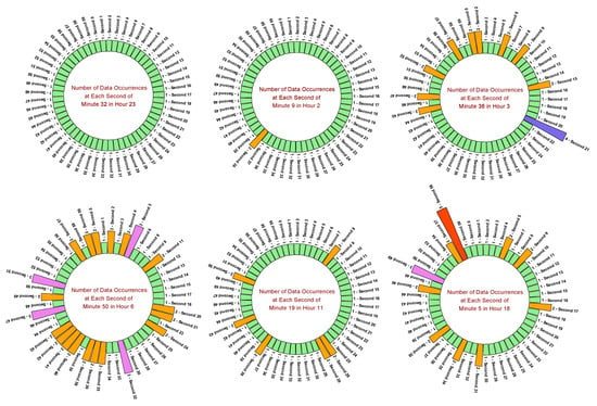
Figure 10.
Occurrence of energy consumption readings at all seconds of various minutes.
From the minute 32 plot, it is observed that there is only 1 occurrence of energy consumption reading at each second, which indicates no redundancy. From the minute 9 plot, it is observed that there is redundancy with 2 occurrences of energy consumption reading at 38th second. From the minute 36 plot, redundancy with 2 occurrences (at seconds 0, 2, 6, 9, 15, 45, 47, 52, 57) and 4 occurrences (at second 21) of energy consumption reading is found. From the minute 50 plot, redundancy with 2 occurrences (at seconds 0, 2, 4, 11, 20, 21, 24, 35, 36, 38, 40, 41, 42, 43, 49, 57, 59) and 3 occurrences (at seconds 5, 32, 47, 51) of energy consumption reading is found.
From the minute 19 plot, it is observed that there is redundancy with 2 occurrences of energy consumption reading at seconds 8, 26, 28, 38, 43, and 50. From the Minute 5 plot, redundancy with 2 occurrences (at seconds 5, 9, 17, 31, 34, 38, 46, 57), 3 occurrences (at second 49), and 5 occurrences (at second 58) of energy consumption reading are found. Hence, from this visualization, it is realized that the redundancy of energy consumption reading at a particular second has been identified mostly with 2 occurrences, moderately with 3 occurrences, and very few with 4 and 5 occurrences.
Additionally, this visualization provides information on missing traces. In line with this, from Figure 10, it is observed that there are no traces of energy consumption reading found at seconds 5, 25, 37 of Minute 32, seconds 28, 43, 49 of Minute 9, seconds 1, 29, 34, 49 of Minute 36, seconds 7, 10, 16, 19, 22, 29, 31, 37, 45 of Minute 50, seconds 18, 27, 52 of Minute 19, seconds 6, 29, 45, 47, 51, 55, 56 of Minute 5. Thus, this analysis unveiled another interesting anomaly of missing traces in smart building energy consumption data.
4.3. Results of Analysis Phase
This visualization is carried out in three steps. The results of the analysis phase produce the result on the types of redundancies (discussed in Section 4.3.1), and the correlation between types of redundancies at the hour level and minute level (discussed in Section 4.3.2).
4.3.1. Analysis of Types of Redundancies
The types of redundancies are expressed as shown in Figure 11, from which, it can be observed that there are two types of redundancies existing in the energy consumption data. The first type of redundancy is “redundancy with same readings”. It can be observed from the upper table of Figure 11, that the READING contains the same readings 164 and 164 at the same timestamp Hour 3 Minute 33 Second 7. The second type of redundancy is “redundancy with different readings”. It can be observed from the lower table of Figure 11, that the READING contains two different readings 171 and 173 at the same timestamp, i.e., Hour 3 Minute 31 Second 24. To further study the number of such types of redundancies that exist in a day, a correlation analysis is executed in Section 4.3.2.

Figure 11.
Types of redundancies identified in the energy consumption data.
4.3.2. Correlation between Types of Redundancies at Hour and Minute Levels
The correlation between the identified two types of redundancies is plotted at the hour level in Figure 12a and at the minute level through Figure 12b–f. For the hour-level analysis, the 24 h (represented as 0 to 23) of a day are taken on the x-axis and the number of redundant traces is taken on the y-axis. Similarly, for minute level analysis, minutes of an hour are taken on the x-axis and the number of redundant traces is taken on the y-axis.
To see the correlation of types of redundancies for the whole day of 26 January 2012, Figure 12a is plotted. From this, it is observed that, out of the total count of redundancies (5060), the count of redundancies with different readings is found to be 3607 and the count of redundancies with the same readings is found to be 1453. Further, it is observed that Hour 3 possesses more redundancies with different readings (247) than the same readings (184) and Hour 6 possesses more redundancies with the same readings (189) than different readings (179). Additionally, this day exhibits an average count of redundancies with different readings as 150 per hour and an average count of redundancies with the same readings as 61 per hour. Similarly, the minute level correlation analysis of types of redundancies is discussed as follows.
- It is evident from Figure 12b that the total count of redundancies observed in Hour 2 is 316, out of which, the count of redundancies with different readings is 198 and the count of same readings is 118. Here, some minutes (1, 6, 8 to 11, 13, 15, 16, 18 to 20, 22 to 24, 27, 29, 30, 42, 58) possess only the redundancies with different readings and all other minutes possess the redundancies of both the types. As a whole in Hour 2, the count of highest redundancies is observed at Minute 57 and the count of lowest redundancies is observed at Minute 9.
- It is evident from Figure 12c that the total count of redundancies observed in Hour 3 is 431, out of which, the count of redundancies with different readings is 247 and those with the same readings is 184. Here, some minutes (44, 48, 49, 55) possess only the redundancies with different readings, some minutes (1, 32) possess only the redundancies with the same readings, and all other minutes possess the redundancies of both types. As a whole in Hour 3, the count of highest redundancies is observed at Minute 16 and the count of lowest redundancies is observed at minutes 48 and 54.
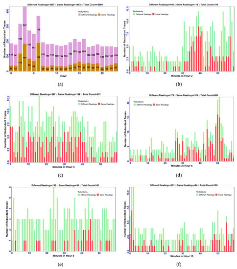 Figure 12. Correlation between the types of redundancies at the hour and minute levels. (a) Correlation between types of redundancies at all Hours. (b) Correlation between types of redundancies at Hour 2. (c) Correlation between types of redundancies at Hour 3. (d) Correlation between types of redundancies at Hour 6. (e) Correlation between types of redundancies at Hour 8. (f) Correlation between types of redundancies at Hour 15.
- It is evident from Figure 12d that the total count of redundancies observed in Hour 6 is 368, out of which, the count of redundancies with different readings is 179 and those with the same readings is 189. Here, some minutes (2 to 5, 7, 8, 10, 14, 15, 19, 23, 35, 41) possess only the redundancies with different readings and all other minutes possess the redundancies of both types. Overall, in Hour 6 the count of highest redundancies is observed at Minute 51 and lowest redundancies is observed at Minute 10.
- It is evident from Figure 12e that the total count of redundancies observed in Hour 8 is 180, out of which, the count of redundancies with different readings is 150 and with the same readings the count is 30. Here, some minutes (0, 1, 3, 4, 6, 9 to13, 18 to 22, 26 to 29, 31, 33 to 35, 37, 39, 47 to 50, 52, 53, 57, 58, 59) possess only the redundancies with different readings and all other minutes possess the redundancies of both the types except minutes 5 and 17. As a whole in Hour 8, the count of highest redundancies is observed at Minute 24 and the count of lowest redundancies (zero) is observed at minutes 5 and 17.
- It is evident from Figure 12f that the total count of redundancies observed in Hour 15 is 195, out of which, the count of redundancies with different readings is 131 and the same readings are 64. Here, some minutes (4, 6, 10, 15 to 17, 20, 21, 24 to 27, 31, 32, 34, 35, 38, 39, 43 to 46, 52, 53) possess only redundancies with different readings, some minutes (11, 54, 58) possess only the redundancies with same readings and all other minutes possess the redundancies of both the types except minute 23. As a whole in Hour 15, the count of highest redundancies is observed at minutes (1, 2) and the count of lowest redundancies (zero) is observed at minute 23.
4.4. Rationale of the Proposed Analytical Enumeration
To validate the usefulness of the proposed analytical enumeration of redundant data anomalies, this section provides a comparison of the proposed approach with a conventional machine learning-based classification approach (named, “random forest”). For this comparison, two test cases are considered, (i) the clean dataset (without redundant energy consumption records) and (ii) the dataset with redundant energy consumption records, as explained in the following subsections.
4.4.1. Test Case-1: Dataset without Redundant Energy Consumption Records
In this case, the conventional and proposed approaches are implemented on a cleaned dataset that is obtained by removing all the identified redundant data records. This clean dataset consists of 78,620 unique records. For the understanding purpose, the confusion matrices are prepared for the results obtained in the case of conventional and proposed approaches as shown in Figure 13. This shows the parity of the existence of redundant and non-redundant records. From these simulations, it is observed that the conventional random forest approach and the proposed analytical enumeration have precisely classified all these 78,620 records as non-redundant. Therefore, from these observations, it is concluded that both conventional and proposed approaches have achieved the same and correct performance when the dataset is clean.

Figure 13.
Comparison of results obtained with conventional and proposed approaches using dataset without redundant energy consumption records.
4.4.2. Test Case-2: Dataset with Redundant Energy Consumption Records
In this case, the conventional and proposed approaches are implemented on the original dataset (i.e., the dataset with the redundant data records). This dataset consists of 87,398 records. The confusion matrices are prepared for the results obtained in the case of conventional and proposed approaches as shown in Figure 14.

Figure 14.
Comparison of results obtained with conventional and proposed approaches using the dataset with redundant energy consumption records.
From these simulations, it is observed that the conventional random forest approach has classified 32,117 records as non-redundant and 5957 records as redundant. However, 49,324 records (4231 + 45,093) do not belong to either redundant or non-redundant, as shown in Figure 14a, which remain ambiguous records. On the other hand, the proposed analytical enumeration has classified 77,210 records as non-redundant and 10,188 records as redundant, where there are no ambiguous records, as shown in Figure 14b. Thus, the conventional approach cannot classify all the records perfectly, whereas, the proposed approach can successfully classify all the records as either redundant or non-redundant records.
Further, the analysis is carried out on the identified redundant records to classify them under the categories “redundant record with the same timestamp and same reading” or “redundant record with the same timestamp and different reading”. In this case, the conventional approach leads to the computation of 1845 ambiguous records along with 4094 redundant records with different readings and 18 redundant records with the same readings as shown in Figure 15. However, in the case of the proposed approach, these are precisely classified as 7252 redundant records with different readings and 2936 redundant records with the same readings without leaving any ambiguous records.

Figure 15.
Summary of quantities computed with conventional and proposed approaches using the dataset with redundant energy consumption records.
Therefore, from these observations, it is evident that the proposed approach has successfully enumerated the number of redundancies and types of redundancies simply and precisely when compared to the conventional approach.
5. Conclusions
Having redundant data anomalies leads to inconsistency in the energy consumption details and also increases the overall size of the database captured, thereby leading to inaccurate analytics. Hence, this paper implements an analytical approach based on enumeration to identify all possible redundant data anomalies in the smart building energy consumption data. The salient observations made from the implementation of the proposed study for enumerating redundancies are consolidated as follows.
Observations from the quantification phase:
- From the day level quantification shown in Figure 4, the highest count of redundancies is observed as ‘5060’ on 26 January 2012, and the lowest count of redundancies is observed as ‘89’ on 24 January 2012, respectively.
- From the hour level quantification shown in Figure 5, the highest count of redundancies is observed as ‘431’ at Hour 3, and the lowest count of redundancies is observed as ’162’ at Hours 17 and 23. Further, the average count of redundancies is computed when the hour level is 211.
- From the minute level quantification shown in Figure 6, the highest count of redundancies is observed as ‘13’ at minute 16 and the lowest count of redundancies is observed as ‘2’ at minutes 48 and 54. Further, the average count of redundancies computed at the minute level is 7.
- From Figure 7, on 26 January 2012, it is understood that there are only 14 min out of 1440 where there are no redundancies found. This means that almost 99% of the minutes in the day possess some kind of redundancy. Thus, this shows the importance of finding all the possible redundant data anomalies, which helps to take necessary measures to enhance the quality of data.
Observations from the visualization phase:
- It is observed that the redundancies in energy consumption readings were recorded mostly with 2 occurrences, moderately with 3 occurrences, and very few with 4 and 5 occurrences.
- Through this visualization, along with the redundant reading anomaly, it is also observed that the energy consumption readings are missed at some seconds as given in Figure 10. This is another type of anomaly detected which may cause inconsistency in the data analysis.
Observations from the analysis phase:
- From Figure 11 and Figure 12, it is understood that there are two types of redundancies existing in the energy consumption data, viz., ‘redundancy with same readings’ and ‘redundancy with different readings. Further, it is identified that the maximum count of redundancies with the same readings is 1453 and the redundancies with different readings are 3607 on the considered day.
Hence, the proposed redundancy anomaly study in this paper successfully enumerated all the possible redundant data anomalies in the considered smart buildings’ energy consumption data. This helps in the process of data cleaning, which is typically required to perform accurate analytics, thus take better decisions for energy management in smart buildings. Additionally, the outcome of this analysis helps as a ready reference to suspect the live data in a smart home/building/grid environment for better data analysis. The method and analysis presented in this paper can be used for any similar application. This supports one of the key objectives of “United Nations Sustainable Development Goals (UN SDGs)—SDG 7: Energy” in producing a quality database for various customer services and energy sustainability.
5.1. Implications of the Findings
As discussed, the major findings of this paper are an enumeration of two types of redundancies, namely “redundant energy consumption records with the same timestamp and same reading” and “redundant energy consumption records with the same timestamp and different readings”. The possible theoretical causes and implications of these findings in real-time are given as follows.
- The implication of finding redundant energy consumption records with the same timestamp and same reading:
In energy metering infrastructure, it is desired to have robust and timely communication between smart meters (transmitters) and the data aggregator (receiver). Usually, whenever a packet is sent from the transmitter, the aggregator receives it at the same timestamp and acknowledges this back to the transmitter. However, any congestion in the network due to latencies or communication network failures creates communication interruptions between the transmitter and the receiver, where the receiver is looking for the packet, but the transmitter is unable to send the packet. In such cases, the receiver may reconsider the previously published data for the current timestamp, which leads to the said redundancy.
- The implication of finding redundant energy consumption records with the same timestamp and different readings:
Usually, the smart meters are desired to capture and send the data at specific intervals of time. However, the issues such as meter malfunctioning or glitches, energy thefts, cyber-attacks, etc., lead to inappropriate or multiple data capturing at the same time intervals. This leads to the redundant readings at the same time instants, thus creating the said redundancy.
5.2. Limitation
This research work is designed in view of the smart building/home/grid data as the targeted application. So, the proposed analytical approach can be exclusively applied to numerical data.
5.3. Future Scope
- Statistical analysis can be done using the two databases, one including the redundancies and the second one with cleaned redundancies, to understand the real impact on the analytics due to these redundancies.
- Before applying this proposed approach, it is better to handle all the missing data for better redundancy analysis. So, the addition of missing data imputation as a pre-step to redundancy analysis can be considered one potential future work.
- Machine learning (ML) techniques are already proven effective and widely used in various applications [50,51] which can yield precise results and analysis by using fast and efficient data-driven models/algorithms. However, the complexity of the ML logics became a key constraint in their implementation. Thus, the application of ML techniques with simplified logics for the analysis of energy consumption data can be considered a subject of potential future work. Here, ML techniques can be used for the investigation of a large dataset automatically and address data quality issues. Further, ML can be used for real-time data prediction without any human effort.
- Application of multi-layer feature selection processes [52] can be considered as potential future research on energy consumption datasets for extracting key features to do the user-defined analysis.
Author Contributions
Conceptualization, G.L.K.M.; Data curation, V.P.K.Y.; Formal analysis, V.P.K.Y.; Funding acquisition, G.L.K.M.; Investigation, P.P.K.; Methodology, P.P.K.; Project administration, A.F.; Resources, A.F.; Software, G.L.K.M.; Supervision, G.L.K.M.; Validation, V.P.K.Y.; Visualization, A.F.; Writing—original draft, P.P.K.; Writing—review and editing, V.P.K.Y. All authors have read and agreed to the published version of the manuscript.
Funding
This research was funded by VIT-AP University, Amaravati, Andhra Pradesh, India.
Institutional Review Board Statement
Not applicable.
Informed Consent Statement
Not applicable.
Data Availability Statement
Not applicable.
Acknowledgments
The authors would like to thank VIT-AP University, Amaravati, Andhra Pradesh, India for funding the open access publication fee for this research work.
Conflicts of Interest
The authors declare no conflict of interest.
References
- Kumar, Y.V.P.; Rao, S.N.V.B.; Padma, K.; Reddy, C.P.; Pradeep, D.J.; Flah, A.; Kraiem, H.; Jasiński, M.; Nikolovski, S. Fuzzy Hysteresis Current Controller for Power Quality Enhancement in Renewable Energy Integrated Clusters. Sustainability 2022, 14, 4851. [Google Scholar] [CrossRef]
- Zielonka, A.; Wozniak, M.; Garg, S.; Kaddoum, G.; Piran, J.; Muhammad, G. Smart Homes: How Much Will They Support Us? A Research on Recent Trends and Advances. IEEE Access 2021, 9, 26388–26419. [Google Scholar] [CrossRef]
- Kasaraneni, P.P.; Yellapragada Venkata, P.K. Simple and Effective Descriptive Analysis of Missing Data Anomalies in Smart Home Energy Consumption Readings. J. Energy Syst. 2021, 5, 199–200. [Google Scholar] [CrossRef]
- Kasaraneni, P.P.; Yellapragada Venkata, P.K. Analytical Approach to Exploring the Missing Data Behavior in Smart Home Energy Consumption Dataset. JREE 2022, 9, 37–48. [Google Scholar] [CrossRef]
- Prakash, K.P.; Kumar, Y.P. A Systematic Approach for Exploration, Behavior Analysis, and Visualization of Redundant Data Anomalies in Smart Home Energy Consumption Dataset. IJRER 2022, 12, 109–123. [Google Scholar] [CrossRef]
- Schuelke-Leech, B.-A.; Barry, B.; Muratori, M.; Yurkovich, B.J. Big Data Issues and Opportunities for Electric Utilities. Renew. Sustain. Energy Rev. 2015, 52, 937–947. [Google Scholar] [CrossRef]
- Firmani, D.; Mecella, M.; Scannapieco, M.; Batini, C. On the Meaningfulness of “Big Data Quality” (Invited Paper). Data Sci. Eng. 2016, 1, 6–20. [Google Scholar] [CrossRef]
- Janssen, M.; van der Voort, H.; Wahyudi, A. Factors Influencing Big Data Decision-Making Quality. J. Bus. Res. 2017, 70, 338–345. [Google Scholar] [CrossRef]
- Peker, N.; Kubat, C. A Hybrid Modified Deep Learning Data Imputation Method for Numeric Datasets. IJISAE 2021, 9, 6–11. [Google Scholar] [CrossRef]
- Sun, L.; Zhou, K.; Zhang, X.; Yang, S. Outlier Data Treatment Methods toward Smart Grid Applications. IEEE Access 2018, 6, 39849–39859. [Google Scholar] [CrossRef]
- Chen, W.; Zhou, K.; Yang, S.; Wu, C. Data Quality of Electricity Consumption Data in a Smart Grid Environment. Renew. Sustain. Energy Rev. 2017, 75, 98–105. [Google Scholar] [CrossRef]
- Hong, T. Big Data Analytics: Making the Smart Grid Smarter [Guest Editorial]. IEEE Power Energy Mag. 2018, 16, 12–16. [Google Scholar] [CrossRef]
- Wang, Y.; Chen, Q.; Hong, T.; Kang, C. Review of Smart Meter Data Analytics: Applications, Methodologies, and Challenges. IEEE Trans. Smart Grid 2019, 10, 3125–3148. [Google Scholar] [CrossRef]
- Pau, M.; Ponci, F.; Monti, A. Analysis of bad data detection capabilities through smart meter based state estimation. In Proceedings of the 2018 IEEE International Conference on Environment and Electrical Engineering and 2018 IEEE Industrial and Commercial Power Systems Europe (EEEIC/I&CPS Europe), Palermo, Italy, 12–15 June 2018; pp. 1–6. [Google Scholar] [CrossRef]
- Yen, S.W.; Morris, S.; Ezra, M.A.G.; Jun Huat, T. Effect of Smart Meter Data Collection Frequency in an Early Detection of Shorter-Duration Voltage Anomalies in Smart Grids. Int. J. Electr. Power Energy Syst. 2019, 109, 1–8. [Google Scholar] [CrossRef]
- Yang, Z.; Liu, H.; Bi, T.; Yang, Q. Bad Data Detection Algorithm for PMU Based on Spectral Clustering. J. Mod. Power Syst. Clean Energy 2020, 8, 473–483. [Google Scholar] [CrossRef]
- Thadikemalla, V.S.G.; Srivastava, I.; Bhat, S.S.; Gandhi, A.S. Data loss mitigation mechanism using compressive sensing for smart grids. In Proceedings of the 2020 IEEE International Conference on Power Electronics, Smart Grid and Renewable Energy (PESGRE2020), Cochin, India, 2–4 January 2020; IEEE: Cochin, India, 2020; pp. 1–6. [Google Scholar] [CrossRef]
- Anwar, A.; Mahmood, A.N. Anomaly Detection in Electric Network Database of Smart Grid: Graph Matching Approach. Electr. Power Syst. Res. 2016, 133, 51–62. [Google Scholar] [CrossRef]
- Elmagarmid, A.K.; Ipeirotis, P.G.; Verykios, V.S. Duplicate Record Detection: A Survey. IEEE Trans. Knowl. Data Eng. 2007, 19, 1–16. [Google Scholar] [CrossRef]
- Leitão, L.; Calado, P.; Herschel, M. Efficient and Effective Duplicate Detection in Hierarchical Data. IEEE Trans. Knowl. Data Eng. 2013, 25, 1028–1041. [Google Scholar] [CrossRef] [Green Version]
- Papenbrock, T.; Heise, A.; Naumann, F. Progressive Duplicate Detection. IEEE Trans. Knowl. Data Eng. 2015, 27, 1316–1329. [Google Scholar] [CrossRef]
- Ioannou, E.; Garofalakis, M. Query Analytics over Probabilistic Databases with Unmerged Duplicates. IEEE Trans. Knowl. Data Eng. 2015, 27, 2245–2260. [Google Scholar] [CrossRef]
- Xia, W.; Jiang, H.; Feng, D.; Hua, Y. Similarity and Locality Based Indexing for High Performance Data Deduplication. IEEE Trans. Comput. 2015, 64, 1162–1176. [Google Scholar] [CrossRef]
- Fu, Y.; Xiao, N.; Jiang, H.; Hu, G.; Chen, W. Application-Aware Big Data Deduplication in Cloud Environment. IEEE Trans. Cloud Comput. 2019, 7, 921–934. [Google Scholar] [CrossRef]
- Hildebrandt, K.; Panse, F.; Wilcke, N.; Ritter, N. Large-Scale Data Pollution with Apache Spark. IEEE Trans. Big Data 2020, 6, 396–411. [Google Scholar] [CrossRef]
- Das, S.; Chakravarthy, S. Duplicate Reduction in Graph Mining: Approaches, Analysis, and Evaluation. IEEE Trans. Knowl. Data Eng. 2018, 30, 1454–1466. [Google Scholar] [CrossRef]
- Dong, Y.; Dragut, E.C.; Meng, W. Normalization of Duplicate Records from Multiple Sources. IEEE Trans. Knowl. Data Eng. 2019, 31, 769–782. [Google Scholar] [CrossRef]
- van Gennip, Y.; Hunter, B.; Ma, A.; Moyer, D.; de Vera, R.; Bertozzi, A.L. Unsupervised Record Matching with Noisy and Incomplete Data. Int. J. Data Sci. Anal. 2018, 6, 109–129. [Google Scholar] [CrossRef]
- Alexandropoulos, S.-A.N.; Kotsiantis, S.B.; Vrahatis, M.N. Data Preprocessing in Predictive Data Mining. Knowl. Eng. Rev. 2019, 34, e1. [Google Scholar] [CrossRef]
- Xia, W.; Jiang, H.; Feng, D.; Douglis, F.; Shilane, P.; Hua, Y.; Fu, M.; Zhang, Y.; Zhou, Y. A Comprehensive Study of the Past, Present, and Future of Data Deduplication. Proc. IEEE 2016, 104, 1681–1710. [Google Scholar] [CrossRef]
- ur Rehman, M.H.; Liew, C.S.; Abbas, A.; Jayaraman, P.P.; Wah, T.Y.; Khan, S.U. Big Data Reduction Methods: A Survey. Data Sci. Eng. 2016, 1, 265–284. [Google Scholar] [CrossRef]
- Vargas-Solar, G.; Zechinelli-Martini, J.L.; Espinosa-Oviedo, J.A. Big Data Management: What to Keep from the Past to Face Future Challenges? Data Sci. Eng. 2017, 2, 328–345. [Google Scholar] [CrossRef]
- The Tracebase Data Set. Available online: http://www.tracebase.org (accessed on 8 July 2022).
- Purna Prakash, K.; Pavan Kumar, Y.V.; Reddy, C.P.; Pradeep, D.J.; Flah, A.; Alzaed, A.N.; Al Ahamdi, A.A.; Ghoneim, S.S.M. A Comprehensive Analytical Exploration and Customer Behaviour Analysis of Smart Home Energy Consumption Data with a Practical Case Study. Energy Rep. 2022, 8, 9081–9093. [Google Scholar] [CrossRef]
- Purna Prakash, K.; Pavan Kumar, Y.V. Exploration of Anomalous Tracing of Records in Smart Home Energy Consumption Dataset. ECS Trans. 2022, 107, 18271–18280. [Google Scholar] [CrossRef]
- Himeur, Y.; Alsalemi, A.; Bensaali, F.; Amira, A. Building Power Consumption Datasets: Survey, Taxonomy and Future Directions. Energy Build. 2020, 227, 110404. [Google Scholar] [CrossRef]
- Klemenjak, C.; Reinhardt, A.; Pereira, L.; Makonin, S.; Bergés, M.; Elmenreich, W. Electricity consumption data sets: Pitfalls and opportunities. In Proceedings of the 6th ACM International Conference on Systems for Energy-Efficient Buildings, Cities, and Transportation, New York, NY, USA, 13–14 November 2019; ACM: New York, NY, USA, 2019; pp. 159–162. [Google Scholar] [CrossRef]
- Moreno Jaramillo, A.F.; Laverty, D.M.; Morrow, D.J.; Martinez del Rincon, J.; Foley, A.M. Load Modelling and Non-Intrusive Load Monitoring to Integrate Distributed Energy Resources in Low and Medium Voltage Networks. Renew. Energy 2021, 179, 445–466. [Google Scholar] [CrossRef]
- Iqbal, H.K.; Malik, F.H.; Muhammad, A.; Qureshi, M.A.; Abbasi, M.N.; Chishti, A.R. A Critical Review of State-of-the-Art Non-Intrusive Load Monitoring Datasets. Electr. Power Syst. Res. 2021, 192, 106921. [Google Scholar] [CrossRef]
- Morais, L.R.; Castro, A.R.G. Competitive Autoassociative Neural Networks for Electrical Appliance Identification for Non-Intrusive Load Monitoring. IEEE Access 2019, 7, 111746–111755. [Google Scholar] [CrossRef]
- Rashid, H.; Singh, P.; Stankovic, V.; Stankovic, L. Can Non-Intrusive Load Monitoring Be Used for Identifying an Appliance’s Anomalous Behaviour? Appl. Energy 2019, 238, 796–805. [Google Scholar] [CrossRef] [Green Version]
- Pipattanasomporn, M.; Chitalia, G.; Songsiri, J.; Aswakul, C.; Pora, W.; Suwankawin, S.; Audomvongseree, K.; Hoonchareon, N. CU-BEMS, Smart Building Electricity Consumption and Indoor Environmental Sensor Datasets. Sci. Data 2020, 7, 241. [Google Scholar] [CrossRef]
- Streltsov, A.; Malof, J.M.; Huang, B.; Bradbury, K. Estimating Residential Building Energy Consumption Using Overhead Imagery. Appl. Energy 2020, 280, 116018. [Google Scholar] [CrossRef]
- Dinesh, C.; Makonin, S.; Bajic, I.V. Residential Power Forecasting Using Load Identification and Graph Spectral Clustering. IEEE Trans. Circuits Syst. II 2019, 66, 1900–1904. [Google Scholar] [CrossRef]
- Chen, H.; Wang, Y.-H.; Fan, C.-H. A Convolutional Autoencoder-Based Approach with Batch Normalization for Energy Disaggregation. J. Supercomput. 2021, 77, 2961–2978. [Google Scholar] [CrossRef]
- Gabaldón, A.; Molina, R.; Marín-Parra, A.; Valero-Verdú, S.; Álvarez, C. Residential End-Uses Disaggregation and Demand Response Evaluation Using Integral Transforms. J. Mod. Power Syst. Clean Energy 2017, 5, 91–104. [Google Scholar] [CrossRef]
- Oluwasuji, O.I.; Malik, O.; Zhang, J.; Ramchurn, S.D. Solving the Fair Electric Load Shedding Problem in Developing Countries. Auton. Agent Multi-Agent Syst. 2020, 34, 12. [Google Scholar] [CrossRef]
- Andreas, R.; Paul, B.; Daniel, B.; Matthias, H.; Hristo, C.; Marc, W.; Ralf, S. On the accuracy of appliance identification based on distributed load metering data. In Proceedings of the 2012 Sustainable Internet and ICT for Sustainability (SustainIT), Pisa, Italy, 4–5 October 2012; pp. 1–9. [Google Scholar]
- Paradiso, F.; Paganelli, F.; Giuli, D.; Capobianco, S. Context-Based Energy Disaggregation in Smart Homes. Future Internet 2016, 8, 4. [Google Scholar] [CrossRef]
- Liu, Y.; Guo, B.; Zou, X.; Li, Y.; Shi, S. Machine Learning Assisted Materials Design and Discovery for Rechargeable Batteries. Energy Storage Mater. 2020, 31, 434–450. [Google Scholar] [CrossRef]
- Liu, Y.; Zhao, T.; Ju, W.; Shi, S. Materials Discovery and Design Using Machine Learning. J. Mater. 2017, 3, 159–177. [Google Scholar] [CrossRef]
- Liu, Y.; Wu, J.; Avdeev, M.; Shi, S. Multi-Layer Feature Selection Incorporating Weighted Score-Based Expert Knowledge toward Modeling Materials with Targeted Properties. Adv. Theory Simul. 2020, 3, 1900215. [Google Scholar] [CrossRef] [Green Version]
Publisher’s Note: MDPI stays neutral with regard to jurisdictional claims in published maps and institutional affiliations. |
© 2022 by the authors. Licensee MDPI, Basel, Switzerland. This article is an open access article distributed under the terms and conditions of the Creative Commons Attribution (CC BY) license (https://creativecommons.org/licenses/by/4.0/).