
Personalized Route Recommendation Using F-AHP-Express


Abstract
:1. Introduction
2. Literature Review
2.1. Road Network
Road Capacity Value (RCV)
2.2. Multicriteria Decision Making
2.2.1. Weight Calculation
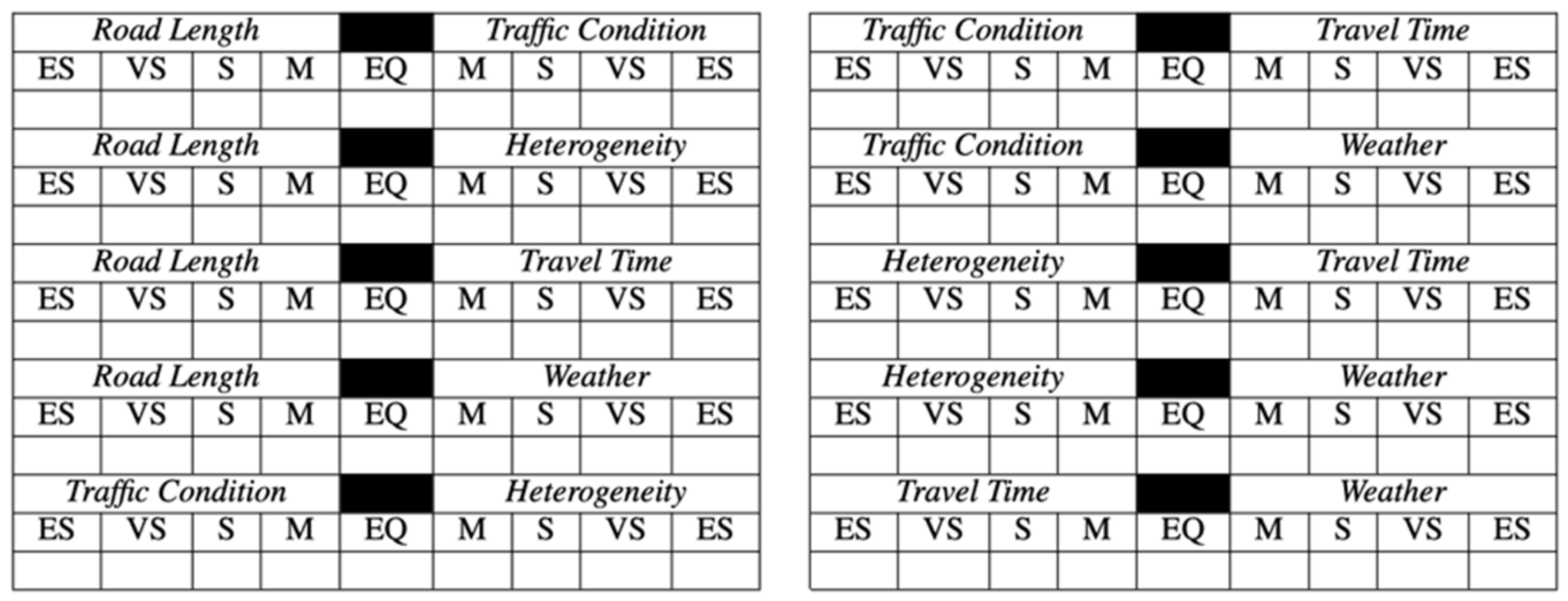
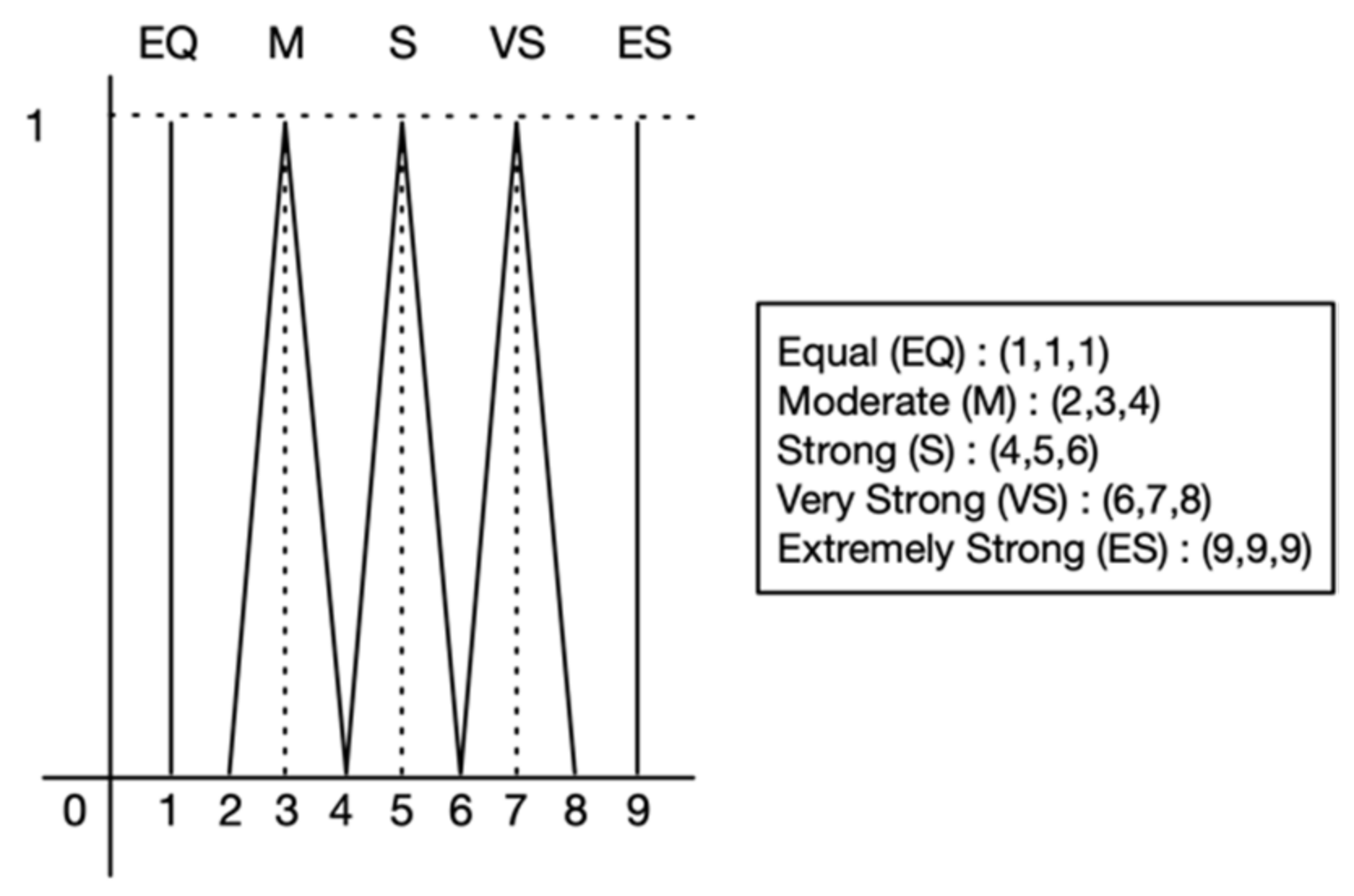
Fuzzy Analytic Hierarchy Process (F-AHP)
2.2.2. Decision Making
Analytics Hierarchy Process
Analytics Hierarchy Process Express
Technique for Others Preference by Similarity to Ideal Solution (TOPSIS)
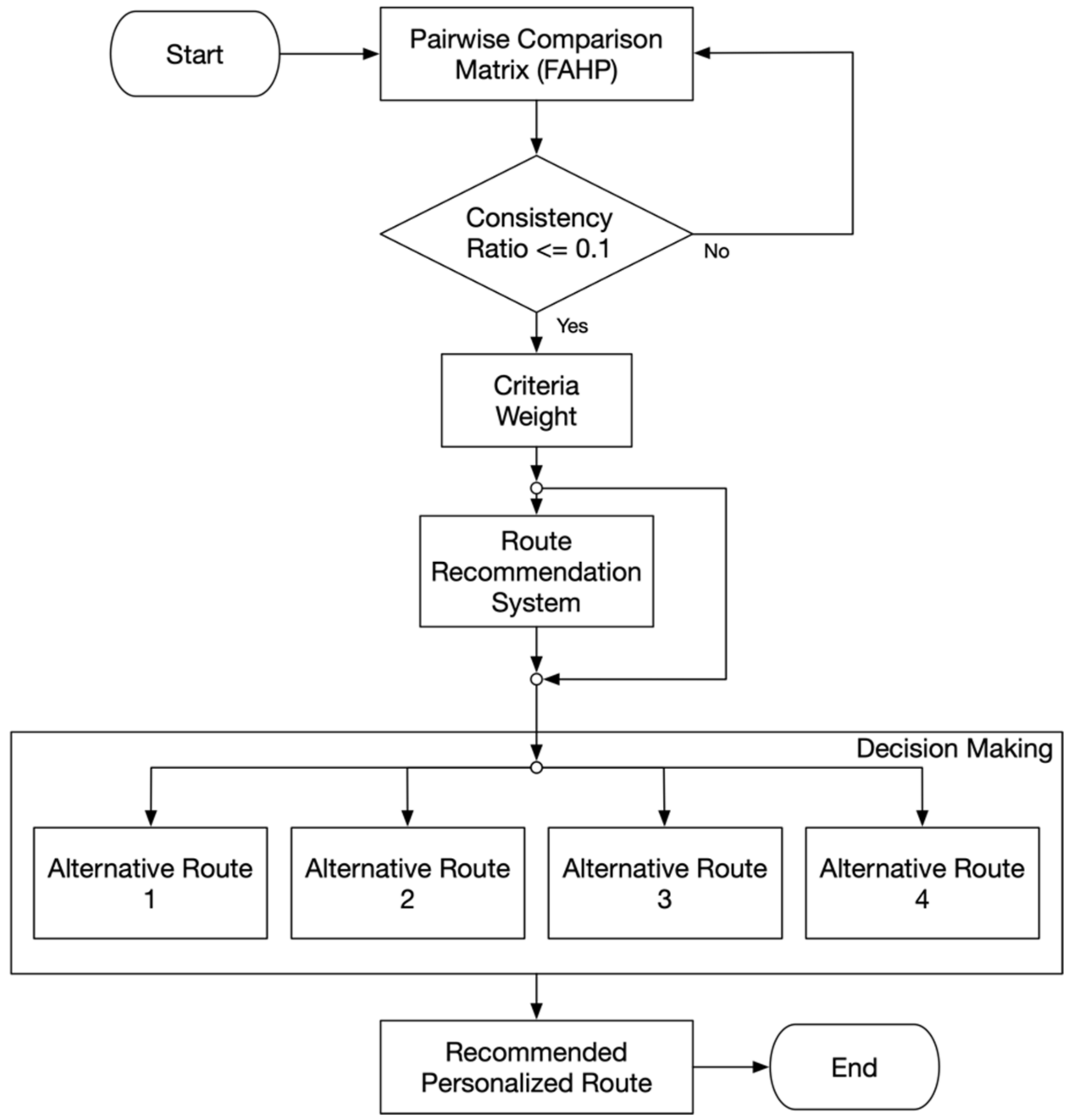
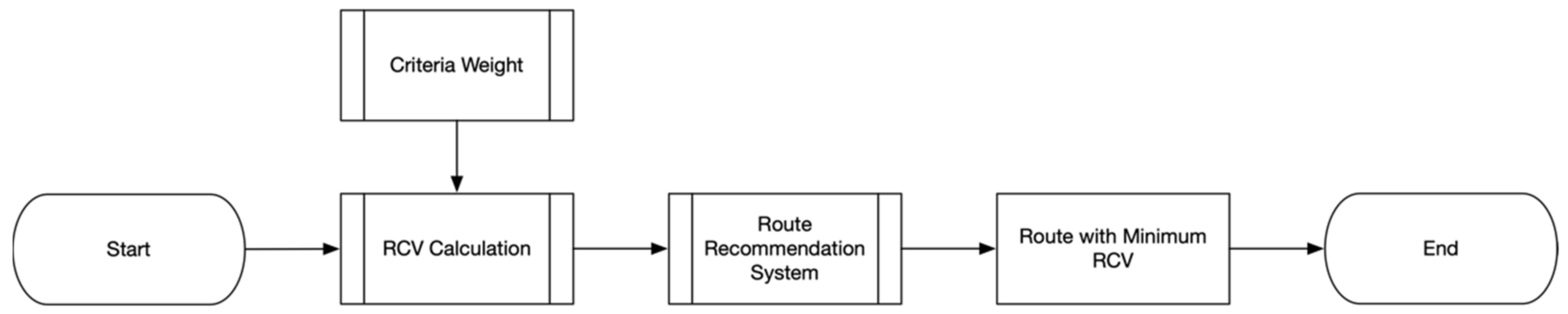
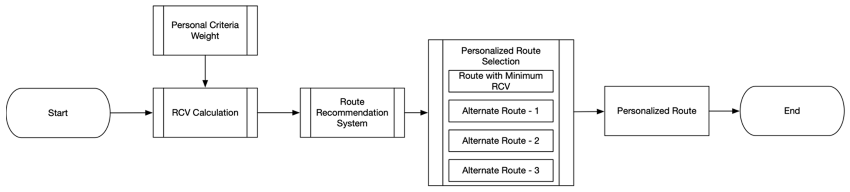
3. Proposed System
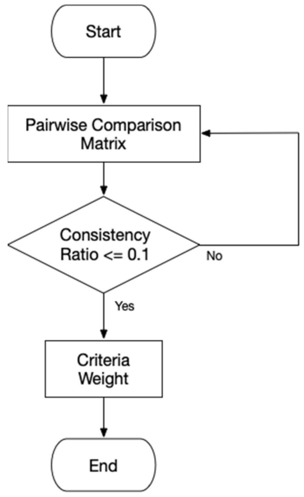
3.1. Calculation of Criteria Weight
3.2. Route Recommendation System
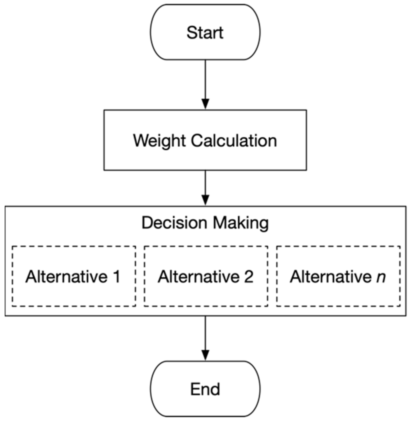
3.3. Decision-Making
4. Results and Discussion
4.1. Weight Calculation
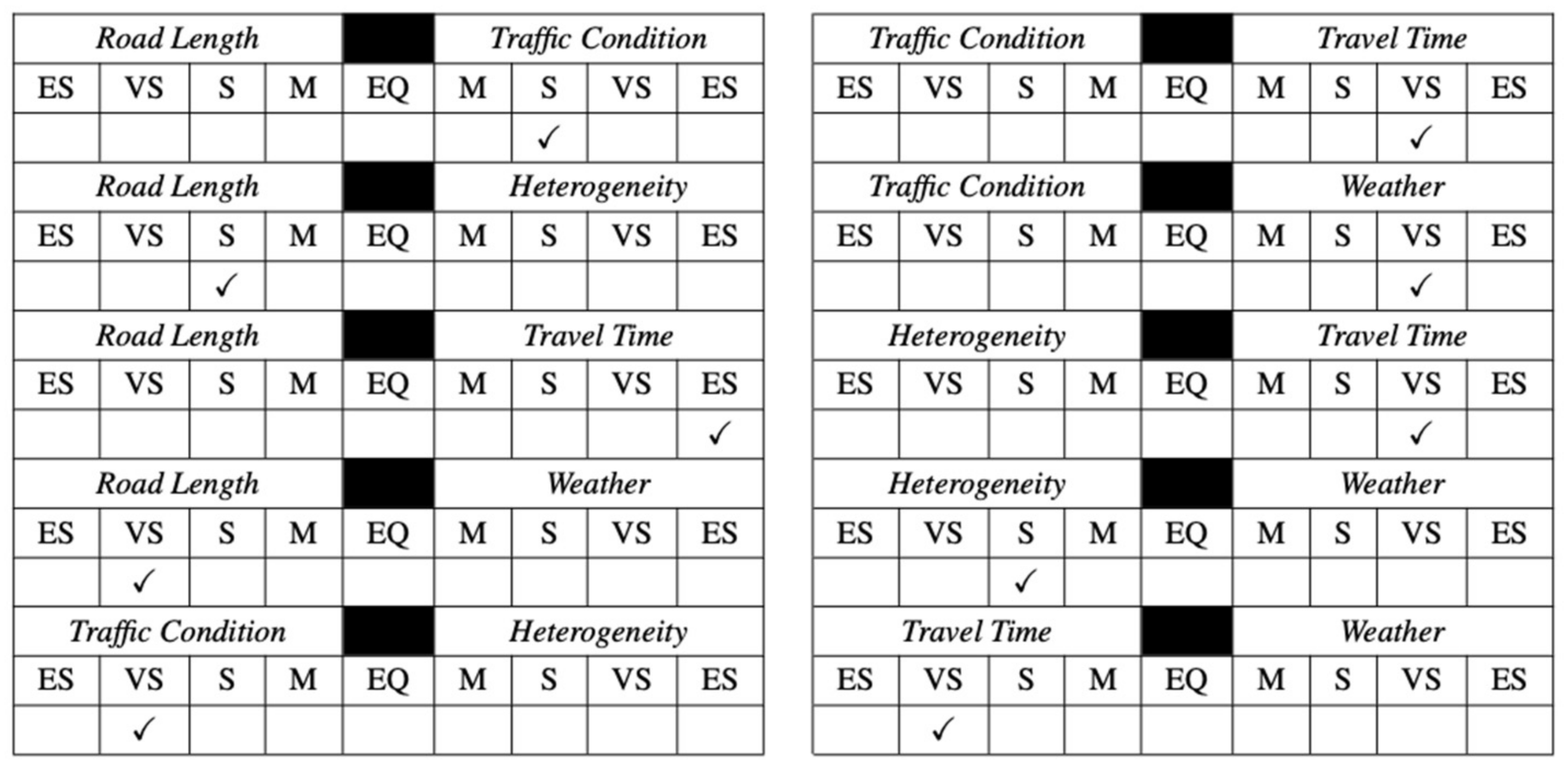
| RL | TC | H | TT | W | RL | TC | H | TT | W | |||
| RL | EQ | S | VS | RL | (1, 1, 1) | (4, 5, 6) | (6, 7, 8) | |||||
| TC | S | EQ | VS | TC | (4, 5, 6) | (1, 1, 1) | (6, 7, 8) | |||||
| H | EQ | S | => | H | (1, 1, 1) | (4, 5, 6) | ||||||
| TT | ES | VS | VS | EQ | VS | TT | (9, 9, 9) | (6, 7, 8) | (6, 7, 8) | (1, 1, 1) | (6, 7, 8) | |
| W | VS | EQ | W | (6, 7, 8) | (1, 1, 1) |
Consistency Ratio Validation for Driver’s Preferences
| RL | TC | H | TT | W | RL | TC | H | TT | W | Average | |||
| RL | 1 | 0.2 | 5 | 0.11 | 7 | RL | 0.07 | 0.01 | 0.25 | 0.07 | 0.35 | 0.15 | |
| TC | 5 | 1 | 7 | 0.14 | 0.14 | TC | 0.33 | 0.07 | 0.35 | 0.09 | 0.01 | 0.17 | |
| H | 0.2 | 0.14 | 1 | 0.14 | 5 | => | H | 0.01 | 0.01 | 0.05 | 0.09 | 0.25 | 0.08 |
| TT | 9 | 7 | 7 | 1 | 7 | TT | 0.59 | 0.46 | 0.35 | 0.65 | 0.35 | 0.48 | |
| W | 0.14 | 7 | 0.2 | 0.14 | 1 | W | 0.01 | 0.46 | 0.01 | 0.09 | 0.05 | 0.12 | |
| Sum | 15.34 | 15.34 | 20.20 | 1.54 | 20.14 |
| RL | TC | H | TT | W | Sum (x’) | |
| RL | 0.15 | 0.03 | 0.41 | 0.05 | 0.87 | 1.51 |
| TC | 0.75 | 0.17 | 0.58 | 0.07 | 0.02 | 1.58 |
| H | 0.03 | 0.02 | 0.08 | 0.07 | 0.62 | 0.82 |
| TT | 1.34 | 1.17 | 0.58 | 0.48 | 0.87 | 4.43 |
| W | 0.02 | 1.17 | 0.02 | 0.07 | 0.12 | 1.40 |
| RL | TC | H | TT | W | RL | TC | H | TT | W | |||
| RL | 1 | 0.2 | 5 | 0.11 | 7 | RL | 1 | 0.33 | 0.33 | 0.14 | 0.33 | |
| TC | 5 | 1 | 7 | 0.14 | 0.14 | TC | 3 | 1 | 0.33 | 0.14 | 0.33 | |
| H | 0.2 | 0.14 | 1 | 0.14 | 5 | => | H | 3 | 3 | 1 | 0.20 | 3 |
| TT | 9 | 7 | 7 | 1 | 7 | TT | 7 | 7 | 5 | 1 | 7 | |
| W | 0.14 | 7 | 0.2 | 0.14 | 1 | W | 3 | 3 | 0.33 | 0.14 | 1 |
| RL | TC | H | TT | W | |
| RL | (1, 1, 1) | (4, 5, 6) | (6, 7, 8) | ||
| TC | (4, 5, 6) | (1, 1, 1) | (6, 7, 8) | ||
| H | (1, 1, 1) | (4, 5, 6) | |||
| TT | (9, 9, 9) | (6, 7, 8) | (6, 7, 8) | (1,1,1) | (6, 7, 8) |
| W | (6, 7, 8) | (1, 1, 1) |
4.2. Decision Making
4.2.1. Analytic Hierarchy Process (AHP)
| RL | TC | H | TT | W | Criteria Weight | Alternative Priority | |||||
| Route-1 | 0.318 | 0.32 | 0.060 | 0.328 | 0.25 | . | RL | 0.049 | Route-1 | 0.269 | |
| Route-2 | 0.534 | 0.04 | 0.151 | 0.540 | 0.25 | TC | 0.082 | Route-2 | 0.393 | ||
| Route-3 | 0.093 | 0.32 | 0.638 | 0.069 | 0.25 | H | 0.182 | = | Route-3 | 0.216 | |
| Route-4 | 0.055 | 0.32 | 0.151 | 0.064 | 0.25 | TT | 0.566 | Route-4 | 0.123 | ||
| W | 0.121 |
4.2.2. Analytic Hierarchy Process—Express (AHP-Express)
| RL | TC | H | TT | W | Criteria Weight | Alternative Priority | |||||
| Route-1 | 0.353 | 0.32 | 0.045 | 0.375 | 0.25 | . | RL | 0.049 | Route-1 | 0.294 | |
| Route-2 | 0.471 | 0.04 | 0.136 | 0.5 | 0.25 | TC | 0.082 | Route-2 | 0.364 | ||
| Route-3 | 0.118 | 0.32 | 0.682 | 0.062 | 0.25 | H | 0.182 | = | Route-3 | 0.221 | |
| Route-4 | 0.059 | 0.32 | 0.136 | 0.062 | 0.25 | TT | 0.566 | Route-4 | 0.119 | ||
| W | 0.121 |
4.2.3. Technique for Others Preference by Similarity to Ideal Solution (TOPSIS)
| Alternatives | RL | TC | H | TT | W | Alternatives | RL | TC | H | TT | W | |
| 1 | 8,225,424 | 3.61 | 9 | 140,379.108 | 0.25 | 1 | 0.483 | 0.455 | 0.525 | 0.477 | 0.5 | |
| 2 | 7,177,041 | 6.25 | 8.41 | 110,598.814 | 0.25 | 2 | 0.451 | 0.598 | 0.508 | 0.423 | 0.5 | |
| 3 | 9,603,801 | 3.61 | 6.76 | 181,038.336 | 0.25 | => | 3 | 0.522 | 0.455 | 0.455 | 0.541 | 0.5 |
| 4 | 10,240,000 | 4 | 8.463 | 185,813.586 | 0.25 | 4 | 0.539 | 0.479 | 0.509 | 0.548 | 0.5 | |
| Sum | 35,246,266 | 17.47 | 32.633 | 617,829.844 | 1 |
| Alternatives | RL | TC | H | TT | W |
| 1 | 0.024 | 0.037 | 0.096 | 0.270 | 0.61 |
| 2 | 0.022 | 0.059 | 0.092 | 0.239 | 0.61 |
| 3 | 0.026 | 0.037 | 0.083 | 0.306 | 0.61 |
| 4 | 0.026 | 0.039 | 0.093 | 0.310 | 0.61 |
4.3. Personal Route Recommendation Analysis
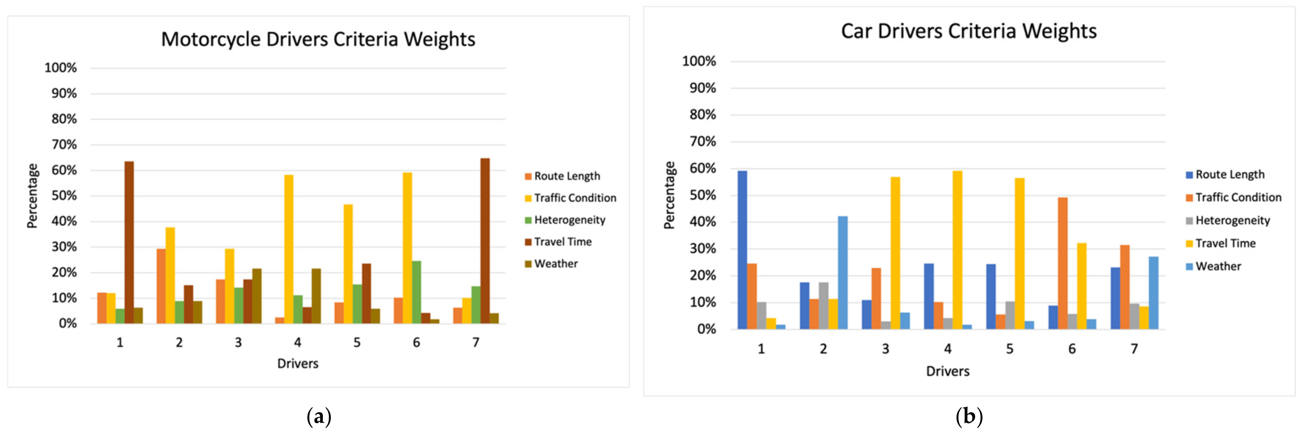
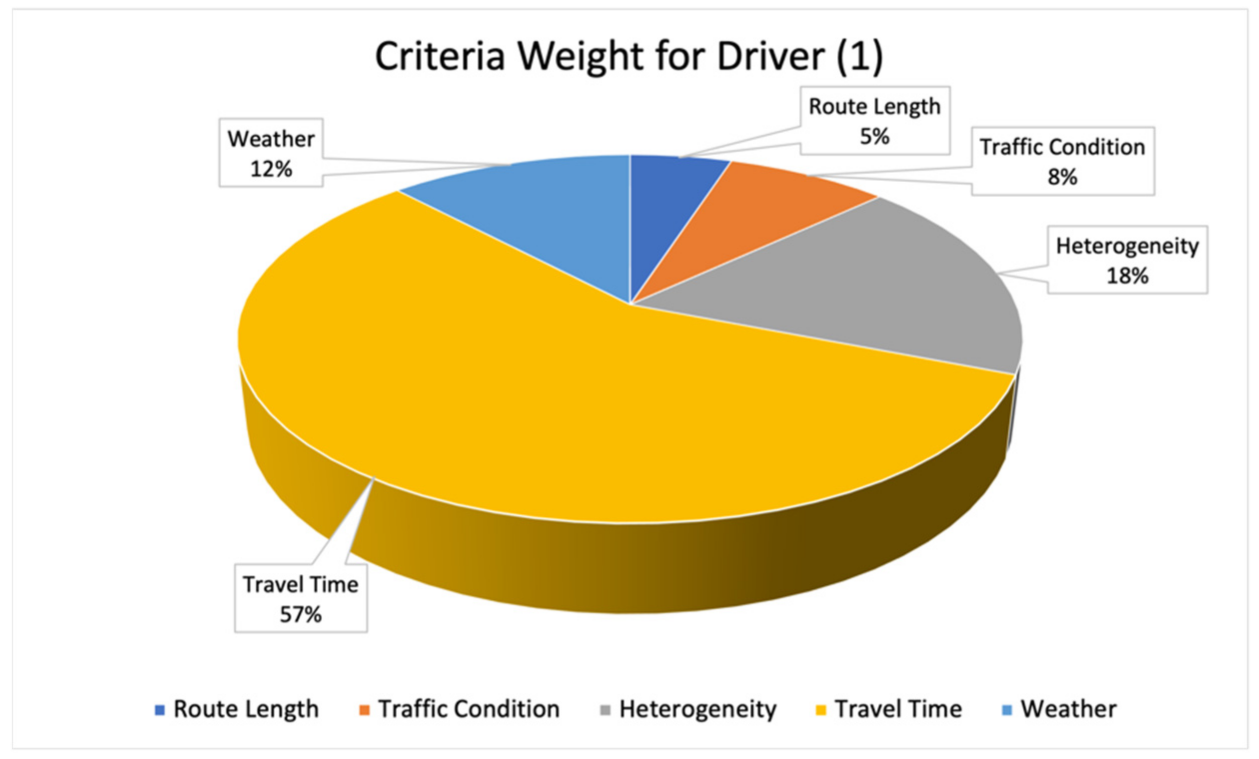
4.3.1. Driver’s Criteria Weight
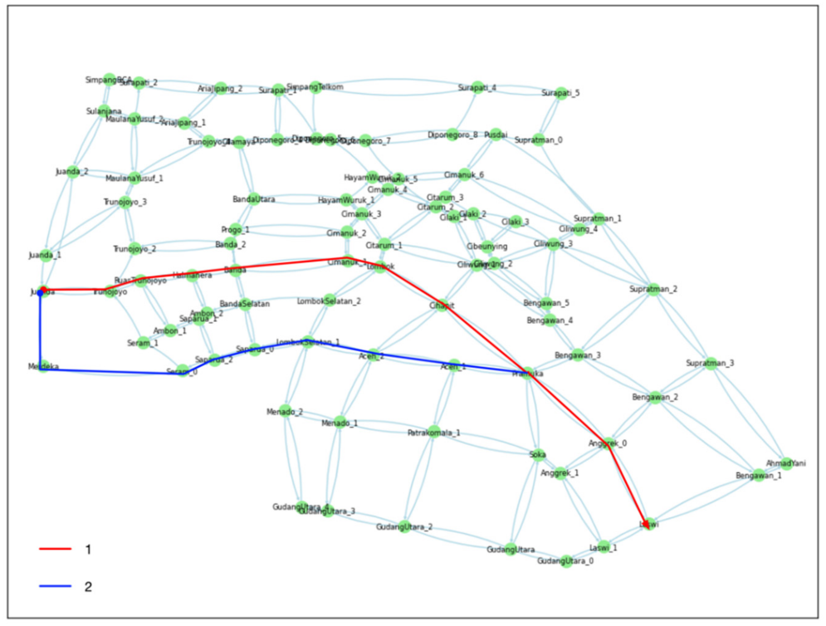
4.3.2. Personal Route Recommendation
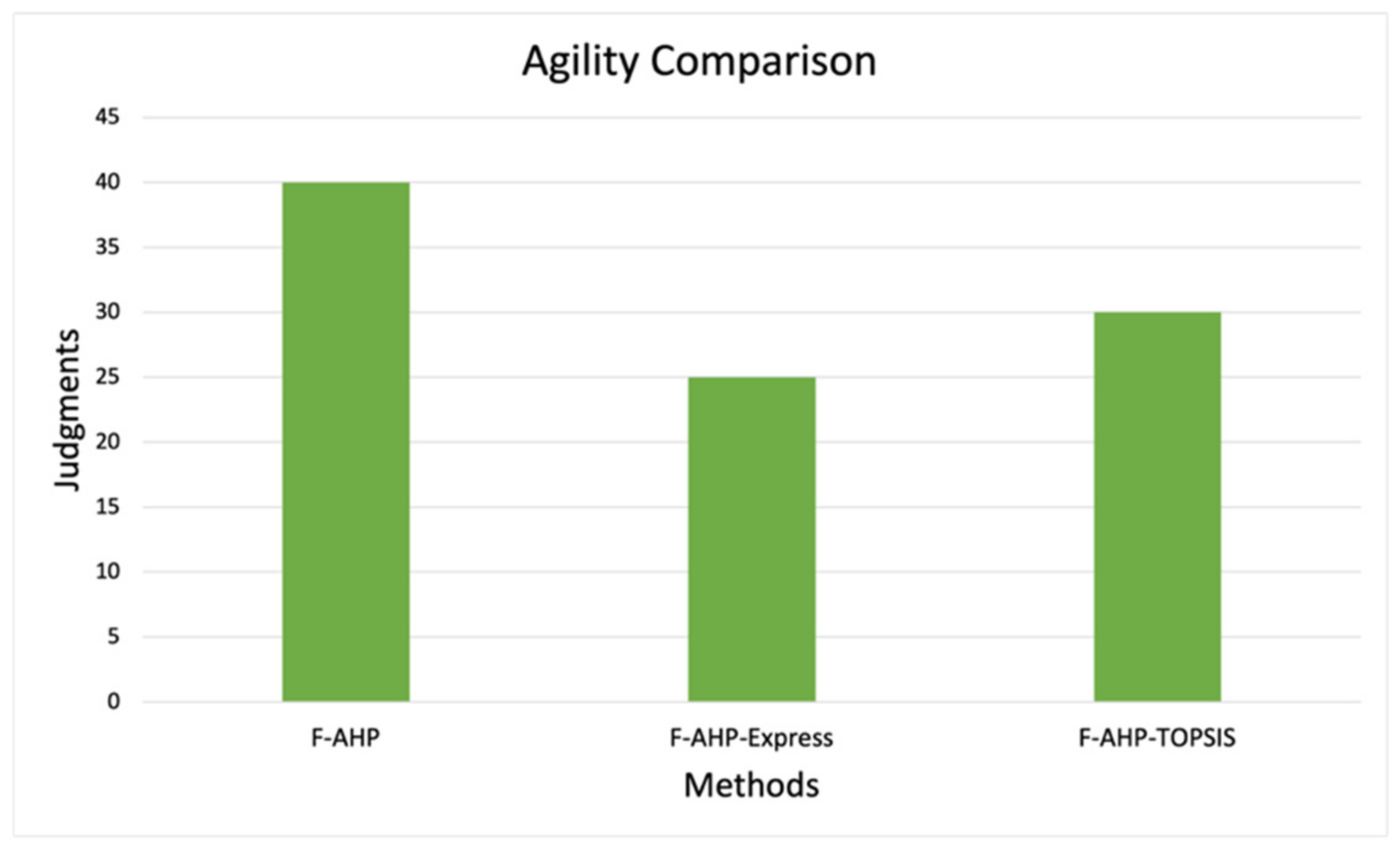
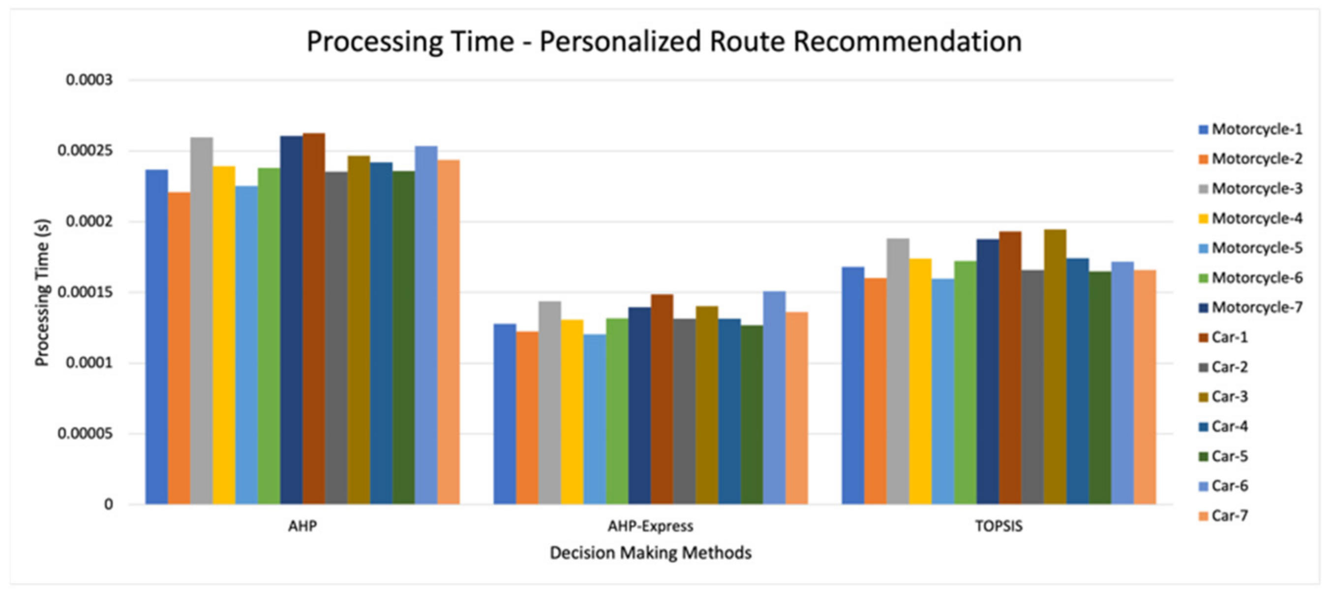
4.3.3. Agility Comparison
4.3.4. Decision-Making Complexity
5. Conclusions
Author Contributions
Funding
Institutional Review Board Statement
Informed Consent Statement
Data Availability Statement
Conflicts of Interest
References
- Balioti, V.; Tzimopoulos, C.; Evangelides, C. Multi Criteria Decision Making Using TOPSIS Method Under Fuzzy Environment. Application in Spillway Selection. Proceedings 2018, 2, 637. [Google Scholar]
- Xiang, Q.J.; Ma, Y.F.; Lu, J. Optimal Route Selection in Highway Network Based on Travel Decision Making. In Proceedings of the 2007 IEEE Intelligent Vehicles Symposium, Istanbul, Turkey, 13–15 June 2007; pp. 1266–1270. [Google Scholar] [CrossRef]
- da Silva, R.F.; Bellinello, M.M.; de Souza, G.F.M.; Antomarioni, S.; Bevilacqua, M.; Ciarapica, F.E. Deciding a Multicriteria Decision-Making (MCDM) Method to Prioritize Maintenance Work Orders of Hydroelectric Power Plants. Energies 2021, 14, 8281. [Google Scholar] [CrossRef]
- Mardani, A.; Jusoh, A.; Nor, K.M.D.; Khalifah, Z.; Zakwan, N.; Valipour, A. Multiple Criteria Decision-Making Techniques and Their Applications—A Review of The Literature from 2000 to 2014. Econ. Res. 2015, 28, 516–571. [Google Scholar] [CrossRef]
- Eltarabishi, F.; Omar, O.H.; Alsyouf, I.; Bettayeb, M. Multi-Criteria Decision Making Methods and Their Applications—A Literature Review. In Proceedings of the International Conference on Industrial Engineering and Operations Management, Detroit, MI, USA, 10–12 March 2020. [Google Scholar]
- Saaty, T.L. Fundamentals of the Analytic Hierarchy Process. In The Analytic Hierarchy Process in Natural Resource and Environmental Decision Making; Springer: Dordrecht, The Netherlands, 2001; pp. 15–35. [Google Scholar] [CrossRef]
- Saaty, T.L. Decision Making with The Analytic Hierarchy Process. Int. J. Serv. Sci. 2008, 1, 83–98. [Google Scholar] [CrossRef]
- Helmy, S.E.; Eladl, G.H.; Eisa, M. Fuzzy Analytical Hierarchy Process (FAHP) Using Geometric Mean Method to Select Best Processing Framework Adequate to Big Data. J. Theor. Appl. Inf. Technol. 2021, 99, 20. [Google Scholar]
- Aliyev, R.; Temizkan, H.; Aliyev, R. Fuzzy Analytic Hierarchy Process-Based Multi-Criteria Decision Making for Universities Ranking. Symmetry 2020, 12, 1351. [Google Scholar] [CrossRef]
- Leal, J.E. AHP-Express: A Simplified Version of The Analytical Hierarchy Process Method. MethodX 2020, 7, 100748. [Google Scholar] [CrossRef]
- Kaya, T.; Kahraman, C. Multicriteria Decision Making in Energy Planning Using a Modified Fuzzy TOPSIS Methodology. Expert Syst. Appl. 2011, 38, 6577–6585. [Google Scholar] [CrossRef]
- Vinodh, S.; Mulanjur, G.; Thiagarajan, A. Sustainable Concept Selection Using Modified Fuzzy TOPSIS: A Case Study. Int. J. Sustain. Eng. 2013, 6, 109–116. [Google Scholar] [CrossRef]
- Chakraborty, S. TOPSIS and Modified TOPSIS: A Comparative Analysis. Decis. Anal. J. 2022, 2, 100021. [Google Scholar] [CrossRef]
- Alhabo, M.; Zhang, L. Multi-Criteria Handover Using Modified Weighted TOPSIS Methods for Heterogeneous Networks. IEEE Access 2018, 6, 40547–40558. [Google Scholar] [CrossRef]
- Kuo, T. A Modified TOPSIS with a Different Ranking Index. Eur. J. Oper. Res. 2017, 260, 152–160. [Google Scholar] [CrossRef]
- García-Cascales, M.S.; Lamata, M.T. On Rank Reversal and TOPSIS Method. Math. Comput. Model. 2012, 56, 123–132. [Google Scholar] [CrossRef]
- Hendawi, A.M.; Rustum, A.; Ahmadain, A.A.; Hazel, D.; Teredesai, A.; Oliver, D.; Ali, M.; Stankovic, J.A. Smart Personalized Routing for Smart Cities. In Proceedings of the 2017 IEEE 33rd International Conference on Data Engineering (ICDE), San Diego, CA, USA, 19–22 April 2017; pp. 1295–1306. [Google Scholar] [CrossRef]
- Chang, G.; Wang, S.; Xiao, X. Review of Spatio-Temporal Models for Short-Term Traffic Forecasting. In Proceedings of the 2016 IEEE International Conference on Intelligent Transportation Engineering (ICITE 2016), Singapore, 20–22 August 2016; pp. 8–12. [Google Scholar] [CrossRef]
- Dauwels, J.; Aslam, A.; Asif, M.T.; Zhao, X.; Mitrovic, N.; Cichocki, A.; Jaillet, P. Predicting Traffic Speed in Urban Transportation Subnetworks for Multiple Horizons. In Proceedings of the 2014 13th International Conference on Control Automation Robotics & Vision (ICARCV), Singapore, 10–12 December 2014. [Google Scholar]
- Nasution, S.M.; Husni, E. Kuspriyanto the Effect of Heterogeneous Traffic Flow on the Transportation System. In Proceedings of the 2018 International Conference on Electrical Engineering, Computing Science, Mexico City, Mexico, 12–14 November 2008; Volume 1. [Google Scholar]
- Kponyo, J.; Kung, Y.; Zhang, E. Dynamic Travel Path Optimization System Using Ant Colony Optimization. In Proceedings of the 2014 UKSim—AMSS 16th International Conference on Computer Modelling and Simulation, Cambridge, UK, 26–28 March 2014; pp. 142–147. [Google Scholar] [CrossRef]
- George, B.; Kim, S. Spatio-Temporal Networks Modeling and Algorithms; Briefs in Computer Science; Springer: New York, NY, USA, 2013. [Google Scholar]
- Ge, Y.; Li, H.; Tuzhilin, A. Route Recommendations for Intelligent Transportation Services. IEEE Trans. Knowl. Data Eng. 2021, 33, 1169–1182. [Google Scholar] [CrossRef]
- Ferreira, H.; Rodrigues, C.M.; Pinho, C. Impact of Road Geometry on Vehicle Energy Consumption and CO2 Emissions: An Energy-Efficiency Rating Methodology. Energies 2019, 13, 119. [Google Scholar] [CrossRef]
- Namoun, A.; Tufail, A.; Mehandjiev, N.; Alrehaili, A.; Akhlaghinia, J.; Peytchev, E. An Eco-Friendly Multimodal Route Guidance System for Urban Areas Using Multi-Agent Technology. Appl. Sci. 2021, 11, 2057. [Google Scholar] [CrossRef]
- Paiva, S.; Pañeda, X.G.; Corcoba, V.; García, R.; Morán, P.; Pozueco, L.; Valdés, M.; Del Camino, C. User Preferences in the Design of Advanced Driver Assistance Systems. Sustainability 2021, 13, 3932. [Google Scholar] [CrossRef]
- Litzinger, P.; Navratil, G.; Sivertun, Å.; Knorr, D. Using Weather Information to Improve Route Planning. In Bridging the Geographic Information Sciences. Lecture Notes in Geoinformation and Cartography; Gensel, J., Josselin, D., Vandenbroucke, D., Eds.; Springer: Berlin/Heidelberg, Germany, 2012; pp. 199–214. [Google Scholar] [CrossRef]
- Bin, C.; Gu, T.; Sun, Y.; Chang, L.; Sun, L. A Travel Route Recommendation System Based on Smart Phones and IoT Environment. Wirel. Commun. Mob. Comput. 2019, 2019, 7038259. [Google Scholar] [CrossRef]
- Das, P.; Ribas-Xirgo, L. Parameter Estimation for Optimal Path Planning in Internal Transportation. arXiv 2018, arXiv:1808.00522. [Google Scholar]
- Kazhaev, A.; Almetova, Z.; Shepelev, V.; Shubenkova, K. Modelling Urban Route Transport Network Parameters with Traffic, Demand and Infrastructural Limitations Being Considered. In IOP Conference Series: Earth and Environmental Science; IOP Publishing: Bristol, UK, 2018; Volume 177. [Google Scholar] [CrossRef]
- Sayarshad, H.R.; Mahmoodian, V.; Bojović, N. Dynamic Inventory Routing and Pricing Problem with a Mixed Fleet of Electric and Conventional Urban Freight Vehicles. Sustainability 2021, 13, 6703. [Google Scholar] [CrossRef]
- Nasution, S.M.; Husni, E.; Kuspriyanto, K.; Yusuf, R.; Yahya, B.N. Contextual Route Recommendation System in Heterogeneous Traffic Flow. Sustainability 2021, 13, 13191. [Google Scholar] [CrossRef]
- Jung, J.; Park, S.; Kim, Y.; Park, S. Route Recommendation with Dynamic User Preference on Road Networks. In Proceedings of the 2019 IEEE International Conference on Big Data and Smart Computing (BigComp), Kyoto, Japan, 27 February 2019–2 March 2019; pp. 1–7. [Google Scholar]
- Shenpei, Z.; Xinping, Y. Driver’s Route Choice Model Based on Traffic Signal Control. In Proceedings of the 2008 3rd IEEE Conference on Industrial Electronics and Applications, Singapore, 3–5 June 2008; pp. 2331–2334. [Google Scholar] [CrossRef]
- He, Z.; Chen, K.; Chen, X. A Collaborative Method for Route Discovery Using Taxi Drivers’ Experience and Preferences. IEEE Trans. Intell. Transp. Syst. 2018, 19, 2505–2514. [Google Scholar] [CrossRef]
- Rouyendegh, B.D.; Erkan, T.E. Selection of Academic Staff Using The Fuzzy Analytic Hierarchy Process (FAHP): A Pilot Study. Teh. Vjesn. 2012, 19, 923–929. [Google Scholar]
- Odu, G. Weighting Methods for Multi Criteria Decision Making Technique. J. Appl. Sci. Environ. Manag. 2019, 23, 1449. [Google Scholar] [CrossRef]
- Keshavarz-Ghorabaee, M.; Amiri, M.; Zavadskas, E.K.; Turskis, Z.; Antucheviciene, J. Determination of Objective Weights Using a New Method Based on the Removal Effects of Criteria (MEREC). Symmetry 2021, 13, 525. [Google Scholar] [CrossRef]
- Ozcan, E.C.; Unlusoy, S.; Eren, T. A Combined Goal Programming—AHP Approach Supported with TOPSIS for Maintenance Strategy Selection in Hydroelectric Power Plants. Renew. Sustain. Energy Rev. 2017, 78, 1410–1423. [Google Scholar] [CrossRef]
- He, C.; Zhang, Q.; Ren, J.; Li, Z. Combined Cooling Heating and Power Systems: Sustainability Assessment Under Uncertainties. Energy 2017, 139, 755–766. [Google Scholar] [CrossRef]
- Rajak, M.; Shaw, K. Evaluation and Selection of Mobile Health (MHealth) Applications Using AHP and Fuzzy TOPSIS. Technol. Soc. 2019, 59, 923–929. [Google Scholar] [CrossRef]
- Abdel-Malak, F.F.; H. Issa, U.; H.Miky, Y.; Osman, E.A. Applying Decision-Making Techniques to Civil Engineering Projects. Beni-Suef Univ. J. Basic Appl. Sci. 2017, 6, 326–331. [Google Scholar]
- Parezanovic, T.; Tarle, S.P.; Petrovic, N. A Multi-Criteria Decision Making Approach for Evaluating Sustainable City Logistics Measures. In Proceedings of the 5th International Conference Transport and Logistics, Hammamet, Tunisia, 1–3 May 2014. [Google Scholar]
- Kumar, R.R.; Mishra, S.; Kumar, C. Prioritizing The Solution of Cloud Service Selection Using Integrated MCDM Methods Under Fuzzy Environment. J. Supercomput. 2017, 73, 4652–4682. [Google Scholar] [CrossRef]
- Kou, G.; Lin, C. A Cosine Maximization Method for the Priority Vector Derivation in AHP. Eur. J. Oper. Res. 2014, 235, 225–232. [Google Scholar] [CrossRef]
- Nguyen, H.D.; Lo, W.T.; Sheu, R.K. An AHP-Based Recommendation System for Exclusive or Specialty Stores. In Proceedings of the 2011 International Conference on Cyber-Enabled Distributed Computing and Knowledge Discovery, Beijing, China, 10–12 October 2011; pp. 16–23. [Google Scholar] [CrossRef]
- Chou, C.-C.; Yu, K.-W. Application of a New Hybrid Fuzzy AHP Model to the Location Choice. Math. Probl. Eng. 2013, 2013, 12. [Google Scholar] [CrossRef]
- Putra, M.S.D.; Andryana, S.; Fauziah; Gunaryati, A. Fuzzy Analytical Hierarchy Process Method to Determine the Quality of Gemstones. Adv. Fuzzy Syst. 2018, 2018, 6. [Google Scholar]
- Kwong, C.K.; Bai, H. A Fuzzy AHP Approach to The Determination of Importance Weights of Customer Requirements in Quality Function Deployment. J. Intell. Manuf. 2002, 13, 367–377. [Google Scholar] [CrossRef]
- Aggarwal, A.G. Aakash An Innovative B2C E-Commerce Websites Selection Using the ME-OWA and Fuzzy AHP. In Proceedings of the First International Conference on Information Technology and Knowledge Management, Turin, Italy, 22–26 October 2018; Volume 14, pp. 13–19. [Google Scholar]
- Khorramrouz, F.; Kajabadi, N.P.; Galankashi, M.R.; Rafiei, F.M. Application of Fuzzy Analytic Hierarchy Process (FAHP) in Failure Investigation of KnowledgeBased Business Plans. Appl. Sci. 2019, 1, 1386. [Google Scholar]
- Chandak, M.M.A.; Borkar, P. Review on Optimal Route Guidance Using Analytical Hierarchy Process. In Proceedings of the 2015 IEEE 9th International Conference on Intelligent Systems and Control (ISCO), Coimbatore, Indiam, 9–10 January 2015; Volume 9. [Google Scholar]
- Buckley, J.J. Fuzzy Hierarchical Analysis. Fuzzy Sets Syst. 1985, 17, 233–247. [Google Scholar] [CrossRef]
- Zlaugotne, B.; Zihare, L.; Balode, L.; Kalnbalkite, A.; Khabdullin, A.; Blumberga, D. Multi Criteria Decision Analysis Methods Comparison. Environ. Clim. Technol. 2020, 24, 454–471. [Google Scholar] [CrossRef]
- Ghaleb, A.M.; Kaid, H.; Alsamhan, A.; Mian, S.H.; Hidri, L. Assessment and Comparison of Various MCDM Approaches in the Selection of Manufacturing Process. Adv. Mater. Sci. Eng. 2020, 2020, 4039253. [Google Scholar] [CrossRef]
- Nadaban, S.; Dzitac, S.; Dzitac, I. Fuzzy TOPSIS: A General View. Procedia Comput. Sci. 2016, 91, 823–831. [Google Scholar] [CrossRef]
- Hwang, C.-L.; Yoon, K. Multiple Attribute Decision Making Methods and Applications A State-of-the-Art Survey. In Lecture Notes in Economics and Mathematical Systems; Springer: New York, NY, USA, 1981. [Google Scholar]
- Ball, S.; Korukoglu, S. Operating System Selection Using Fuzzy AHP and TOPSIS Methods. Math. Comput. Appl. 2009, 14, 119–130. [Google Scholar] [CrossRef]
- Shafiq, M. Dynamic Route Optimization for Heterogeneous Agent Envisaging Topographic of Maps. EPiC Ser. Eng. 2018, 2, 206–217. [Google Scholar]
- Delling, D.; Sanders, P.; Schultes, D.; Wagner, D. Engineering and Augmenting Route Planning Algorithms. Algorithm. Large Complex Netw. 2009, 5515, 117–139. [Google Scholar]
- Elmahmoudi, F.; El Kheir Abra, O.; Raihani, A.; Serrar, O.; Bahatti, L. GIS Based Fuzzy Analytic Hierarchy Process for Wind Energy Sites Selection in Tarfaya Morocco. In Proceedings of the 2020 IEEE International conference of Moroccan Geomatics (Morgeo), Casablanca, Morocco, 11–13 May 2020. [Google Scholar]
- Meng, W.; Kai, L.; Songhui, Z. Evaluation of Electric Vehicle Charging Station Sitting Based on Fuzzy Analytic Hierarchy Process. In Proceedings of the 2013 Fourth International Conference on Digital Manufacturing & Automation, Shinan, China, 29–30 June 2013. [Google Scholar]
- Jupri, M.; Sarno, R. Data Mining, Fuzzy AHP and TOPSIS for Optimizing Taxpayer Supervision. Indones. J. Electr. Eng. Comput. Sci. 2020, 18, 75–87. [Google Scholar] [CrossRef]


| Method Ranks | [3] | [4] | [5] |
|---|---|---|---|
| 1 | AHP | AHP | Hybrid MCDM |
| 2 | TOPSIS | Hybrid MCDM | AHP |
| 3 | ANP | Aggregate Methods | Aggregate Methods |
| 4 | VIKOR | TOPSIS | TOPSIS |
| 5 | PROMETHEE | ELECTRE | ELECTRE |
| Importance Level | Definition |
|---|---|
| 1 | Equal Importance |
| 3 | Moderate Importance |
| 5 | Strong Importance |
| 7 | Very Strong Importance |
| 9 | Extremely Strong Importance |
| 2, 4, 6, 8 | Intermediate Value between Previous Levels |
| Criteria | Ratio Index | Criteria | Ratio Index |
|---|---|---|---|
| 1 | 0 | 7 | 1.32 |
| 2 | 0 | 8 | 1.41 |
| 3 | 0.58 | 9 | 1.45 |
| 4 | 0.9 | 10 | 1.49 |
| 5 | 1.12 | 11 | 1.51 |
| 6 | 1.24 | 12 | 1.56 |
| RL | 1.51 | 0.15 | 10.15 |
| TC | 1.58 | 0.17 | 9.41 |
| H | 0.82 | 0.08 | 9.96 |
| TT | 4.43 | 0.48 | 9.29 |
| W | 1.40 | 0.12 | 11.35 |
| 10.03 | |||
| 1.26 | |||
| 1.12 | |||
| Alternatives | Travel Routes |
|---|---|
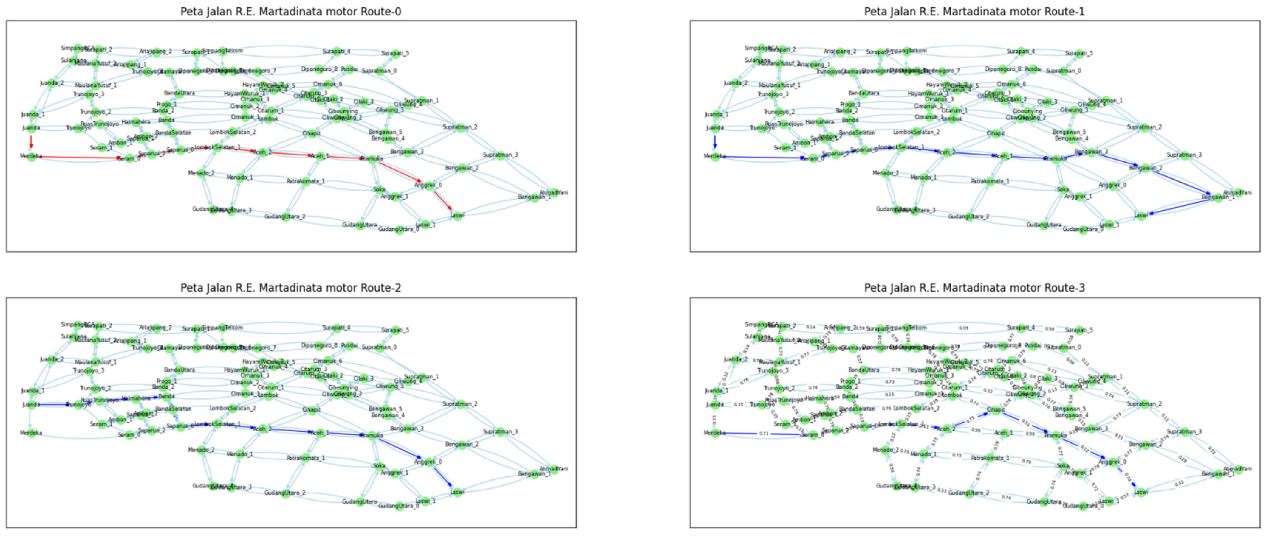
| Route-1 | Juanda-Merdeka-Seram 0-Saparua 2-Saparua 0-LombokSelatan 1-Aceh 2-Aceh 1-Pramuka-Anggrek 0-Laswi |
| Route-2 | Juanda-Trunojoyo-RuasTrunojoyo-Halmahera-Banda-Cimanuk 1-Lombok-Cihapit-Pramuka-Anggrek 0-Laswi |
| Route-3 | Juanda-Merdeka-Seram 0-Saparua 2-Saparua 0-LombokSelatan 1-Aceh 2-Cihapit-Pramuka-Anggrek 0-Laswi |
| Route-4 | Juanda-Merdeka-Seram 0-Saparua 2-Saparua 0-LombokSelatan 1-LombokSelatan 2-Lombok-Cihapit-Pramuka-Anggrek 0-Laswi |
| Alternatives | RL | TC | H | TT | W |
|---|---|---|---|---|---|
| Route-1 | 2868 | 1.9 | 3 | 374.672 | 0.5 |
| Route-2 | 2679 | 2.5 | 2.9 | 332.564 | 0.5 |
| Route-3 | 3099 | 1.9 | 2.6 | 425.486 | 0.5 |
| Route-4 | 3200 | 2.0 | 2.91 | 431.061 | 0.5 |
| RL | Route 1 | Route 2 | Route 3 | Route 4 |
|---|---|---|---|---|
| Route 1 | 1 | 0.5 | 4 | 6 |
| Route 2 | 2 | 1 | 6 | 8 |
| Route 3 | 0.25 | 0.167 | 1 | 2 |
| Route 4 | 0.167 | 0.125 | 0.5 | 1 |
| TC | Route 1 | Route 2 | Route 3 | Route 4 |
| Route 1 | 1 | 8 | 1 | 1 |
| Route 2 | 0.125 | 1 | 0.125 | 0.125 |
| Route 3 | 1 | 8 | 1 | 1 |
| Route 4 | 1 | 8 | 1 | 1 |
| H | Route 1 | Route 2 | Route 3 | Route 4 |
| Route 1 | 1 | 0.33 | 0.125 | 0.33 |
| Route 2 | 3 | 1 | 0.2 | 1 |
| Route 3 | 8 | 5 | 1 | 5 |
| Route 4 | 3 | 1 | 0.2 | 1 |
| TT | Route 1 | Route 2 | Route 3 | Route 4 |
| Route 1 | 1 | 0.5 | 5 | 6 |
| Route 2 | 2 | 1 | 7 | 8 |
| Route 3 | 0.2 | 0.143 | 1 | 1 |
| Route 4 | 0.167 | 0.125 | 1 | 1 |
| W | Route 1 | Route 2 | Route 3 | Route 4 |
| Route 1 | 1 | 1 | 1 | 1 |
| Route 2 | 1 | 1 | 1 | 1 |
| Route 3 | 1 | 1 | 1 | 1 |
| Route 4 | 1 | 1 | 1 | 1 |
| RL | Route 1 | Route 2 | Route 3 | Route 4 | Sum |
|---|---|---|---|---|---|
| Route 4 | 0.167 | 0.125 | 0.5 | 1 | |
| Reciprocal Value | 6 | 8 | 2 | 1 | 17 |
| Normalization | 0.353 | 0.471 | 0.118 | 0.059 | 1 |
| TC | Route 1 | Route 2 | Route 3 | Route 4 | Sum |
| Route 2 | 0.125 | 1 | 0.125 | 0.125 | |
| Reciprocal Value | 8 | 1 | 8 | 8 | 25 |
| Normalization | 0.32 | 0.04 | 0.32 | 0.32 | 1 |
| H | Route 1 | Route 2 | Route 3 | Route 4 | Sum |
| Route 1 | 1 | 0.33 | 0.125 | 0.33 | |
| Reciprocal Value | 1 | 3 | 8 | 3 | 15 |
| Normalization | 0.067 | 0.2 | 0.533 | 0.2 | 1 |
| TT | Route 1 | Route 2 | Route 3 | Route 4 | Sum |
| Route 4 | 0.167 | 0.125 | 1 | 1 | |
| Reciprocal Value | 6 | 8 | 1 | 1 | 16 |
| Normalization | 0.375 | 0.5 | 0.062 | 0.062 | 1 |
| W | Route 1 | Route 2 | Route 3 | Route 4 | Sum |
| Route 3 | 1 | 1 | 1 | 1 | |
| Reciprocal Value | 1 | 1 | 1 | 1 | 4 |
| Normalization | 0.25 | 0.25 | 0.25 | 0.25 | 1 |
| Ideal Value | RL | TC | H | TT | W |
|---|---|---|---|---|---|
| Positive Ideal Value | 0.022 | 0.037 | 0.083 | 0.239 | 0.061 |
| Negative Ideal Value | 0.026 | 0.059 | 0.096 | 0.310 | 0.061 |
| Alternatives | RL | TC | H | TT | W | Positive Ideal Distance (Si+) |
|---|---|---|---|---|---|---|
| 1 | 4 × 10⁻⁶ | 0 | 0.000169 | 0.000961 | 0 | 0.033 |
| 2 | 0 | 0.000484 | 8.1 × 10⁻⁵ | 0 | 0 | 0.015 |
| 3 | 0.000016 | 0 | 0 | 0.004489 | 0 | 0.067 |
| 4 | 0.000016 | 4 × 10⁻⁶ | 1 × 10⁻⁴ | 0.005041 | 0 | 0.072 |
| Alternatives | RL | TC | H | TT | W | Negative Ideal Distance (Si−) |
|---|---|---|---|---|---|---|
| 1 | 4 × 10⁻⁶ | 0.000484 | 0 | 0.0016 | 0 | 0.042 |
| 2 | 0.000016 | 0 | 0.000016 | 0.005041 | 0 | 0.071 |
| 3 | 0 | 0.000484 | 0.000169 | 0.000016 | 0 | 0.018 |
| 4 | 0 | 0.0004 | 9 × 10⁻⁶ | 0 | 0 | 0.010 |
| Alternatives | Positive Ideal Distance (Si+) | Negative Ideal Distance (Si−) | Performance Index (Pi) |
|---|---|---|---|
| 1 | 0.033 | 0.042 | 0.563 |
| 2 | 0.015 | 0.071 | 0.824 |
| 3 | 0.067 | 0.018 | 0.210 |
| 4 | 0.072 | 0.010 | 0.125 |
| Drivers | Vehicle Type | RL | TC | H | TT | W |
|---|---|---|---|---|---|---|
| 1 | Motorcycle | 0.1218 | 0.1201 | 0.0593 | 0.6353 | 0.0634 |
| 2 | Motorcycle | 0.2936 | 0.3774 | 0.0892 | 0.1506 | 0.0892 |
| 3 | Motorcycle | 0.1743 | 0.2937 | 0.1416 | 0.1743 | 0.2161 |
| 4 | Motorcycle | 0.025 | 0.5827 | 0.1114 | 0.0651 | 0.2159 |
| 5 | Motorcycle | 0.0837 | 0.4675 | 0.1543 | 0.2356 | 0.0589 |
| 6 | Motorcycle | 0.1021 | 0.5921 | 0.2459 | 0.0424 | 0.0176 |
| 7 | Motorcycle | 0.0629 | 0.1017 | 0.1467 | 0.6476 | 0.0412 |
| 8 | Car | 0.5921 | 0.2459 | 0.1021 | 0.0424 | 0.0176 |
| 9 | Car | 0.1755 | 0.1131 | 0.1755 | 0.1131 | 0.4227 |
| 10 | Car | 0.1094 | 0.2294 | 0.0295 | 0.5693 | 0.0625 |
| 11 | Car | 0.2459 | 0.1021 | 0.0424 | 0.5921 | 0.0176 |
| 12 | Car | 0.2434 | 0.0554 | 0.1048 | 0.565 | 0.0314 |
| 13 | Car | 0.0884 | 0.493 | 0.0579 | 0.3228 | 0.0379 |
| 14 | Car | 0.2313 | 0.3148 | 0.0965 | 0.0859 | 0.2715 |
| Alternatives | Routes | RL | TC | H | TT | W |
|---|---|---|---|---|---|---|
| 1 | Juanda-Merdeka-Seram0-Saparua2-Saparua0-LombokSelatan1-Aceh2-Aceh1-Pramuka-Anggrek0-Laswi | 2868 | 1.9 | 3 | 374.672 | 0.5 |
| 2 | Juanda-Trunojoyo-RuasTrunojoyo-Halmahera-Banda-Cimanuk1-Lombok-Cihapit-Pramuka-Anggrek0-Laswi | 2679 | 2.5 | 2.9 | 332.564 | 0.5 |
| 3 | Juanda-Merdeka-Seram0-Saparua2-Saparua0-LombokSelatan1-Aceh2-Cihapit-Pramuka-Anggrek0-Laswi | 3099 | 1.9 | 2.6 | 425.486 | 0.5 |
| 4 | Juanda-Merdeka-Seram0-Saparua2-Saparua0-LombokSelatan1-LombokSelatan2-Lombok-Cihapit-Pramuka-Anggrek0-Laswi | 3200 | 2.0 | 2.91 | 431.061 | 0.5 |
| Drivers | AHP | AHP-Express | TOPSIS |
|---|---|---|---|
| Motorcycle-1 | Route-1 | Route-1 | Route-1 |
| Motorcycle-2 | Route-3 | Route-3 | Route-3 |
| Motorcycle-3 | Route-3 | Route-3 | Route-3 |
| Motorcycle-4 | Route-2 | Route-2 | Route-2 |
| Motorcycle-5 | Route-3 | Route-3 | Route-3 |
| Motorcycle-6 | Route-2 | Route-2 | Route-2 |
| Motorcycle-7 | Route-1 | Route-1 | Route-1 |
| Car-1 | Route-1 | Route-1 | Route-1 |
| Car-2 | Route-2 | Route-2 | Route-2 |
| Car-3 | Route-1 | Route-1 | Route-1 |
| Car-4 | Route-1 | Route-1 | Route-1 |
| Car-5 | Route-1 | Route-1 | Route-1 |
| Car-6 | Route-2 | Route-2 | Route-2 |
| Car-7 | Route-2 | Route-2 | Route-2 |
| Drivers | Recommendation | Routes | Group |
|---|---|---|---|
| Motorcycle-1 | Route-1 | Juanda-Trunojoyo-RuasTrunojoyo-Halmahera-Banda-Cimanuk 1-Lombok-Cihapit-Pramuka-Anggrek 0-Laswi | 1 |
| Motorcycle-2 | Route -3 | Juanda-Merdeka-Seram 0-Saparua 2-Saparua 0-LombokSelatan 1-Aceh 2-Aceh 1-Pramuka-Anggrek 0-Laswi | 2 |
| Motorcycle-3 | Route -3 | Juanda-Merdeka-Seram 0-Saparua 2-Saparua 0-LombokSelatan 1-Aceh 2-Aceh 1-Pramuka-Anggrek 0-Laswi | 2 |
| Motorcycle-4 | Route -2 | Juanda-Merdeka-Seram 0-Saparua 2-Saparua 0-LombokSelatan 1-Aceh 2-Aceh 1-Pramuka-Anggrek 0-Laswi | 2 |
| Motorcycle-5 | Route -3 | Juanda-Merdeka-Seram 0-Saparua 2-Saparua 0-LombokSelatan 1-Aceh 2-Aceh 1-Pramuka-Anggrek 0-Laswi | 2 |
| Motorcycle-6 | Route -2 | Juanda-Merdeka-Seram 0-Saparua 2-Saparua 0-LombokSelatan 1-Aceh 2-Aceh 1-Pramuka-Anggrek 0-Laswi | 2 |
| Motorcycle-7 | Route -1 | Juanda-Trunojoyo-RuasTrunojoyo-Halmahera-Banda-Cimanuk 1-Lombok-Cihapit-Pramuka-Anggrek 0-Laswi | 1 |
| Car-1 | Route -1 | Juanda-Merdeka-Seram 0-Saparua 2-Saparua 0-LombokSelatan 1-Aceh 2-Aceh 1-Pramuka-Anggrek 0-Laswi | 2 |
| Car-2 | Route -2 | Juanda-Merdeka-Seram 0-Saparua 2-Saparua 0-LombokSelatan 1-Aceh 2-Aceh 1-Pramuka-Anggrek 0-Laswi | 2 |
| Car-3 | Route -1 | Juanda-Trunojoyo-RuasTrunojoyo-Halmahera-Banda-Cimanuk 1-Lombok-Cihapit-Pramuka-Anggrek 0-Laswi | 1 |
| Car-4 | Route -1 | Juanda-Trunojoyo-RuasTrunojoyo-Halmahera-Banda-Cimanuk 1-Lombok-Cihapit-Pramuka-Anggrek 0-Laswi | 1 |
| Car-5 | Route -1 | Juanda-Trunojoyo-RuasTrunojoyo-Halmahera-Banda-Cimanuk 1-Lombok-Cihapit-Pramuka-Anggrek 0-Laswi | 1 |
| Car-6 | Route -2 | Juanda-Merdeka-Seram 0-Saparua 2-Saparua 0-LombokSelatan 1-Aceh 2-Aceh 1-Pramuka-Anggrek 0-Laswi | 2 |
| Car-7 | Route -2 | Juanda-Merdeka-Seram 0-Saparua 2-Saparua 0-LombokSelatan 1-Aceh 2-Aceh 1-Pramuka-Anggrek 0-Laswi | 2 |
| Multicriteria Decision-Making Methods | |
|---|---|
| F-AHP | |
| F-AHP-Express | |
| F-AHP-TOPSIS |
| Decision Making Methods | Steps | Complexity |
|---|---|---|
| AHP | (1) Alternatives Comparison Based on Criteria (2) Row Summation (3) Normalization (4) Averaging Normalization (5) Decision Making | O(n2) O(n2) O(n2) O(n2) O(n) |
| AHP-Express | (1) Alternative Comparison (One Alternative for each Criteria) (2) Reciprocal Value and Summation (3) Normalization (4) Decision Making | O(n) O(n) O(n) O(n) |
| TOPSIS | (1) Row Summation (2) Normalization (3) Weighted Normalization (4) Positive and Negative Ideal Solution (5) Positive and Negative Ideal Solution Distance (6) Decision Making | O(n2) O(n2) O(n2) O(n2) O(n2) O(n2) |
| Experiments | AHP | AHP-Express | TOPSIS |
|---|---|---|---|
| Processing Time (Decision Making) | 0.000225133 s | 0.000124533 s | 0.000156033 s |
| Agility (Weight Calculation and Decision Making) | 40 judgments | 25 judgments | 30 judgments |
| Complexity (Decision Making) |
Publisher’s Note: MDPI stays neutral with regard to jurisdictional claims in published maps and institutional affiliations. |
© 2022 by the authors. Licensee MDPI, Basel, Switzerland. This article is an open access article distributed under the terms and conditions of the Creative Commons Attribution (CC BY) license (https://creativecommons.org/licenses/by/4.0/).
Share and Cite
Nasution, S.M.; Husni, E.; Kuspriyanto, K.; Yusuf, R. Personalized Route Recommendation Using F-AHP-Express. Sustainability 2022, 14, 10831. https://doi.org/10.3390/su141710831
Nasution SM, Husni E, Kuspriyanto K, Yusuf R. Personalized Route Recommendation Using F-AHP-Express. Sustainability. 2022; 14(17):10831. https://doi.org/10.3390/su141710831
Chicago/Turabian StyleNasution, Surya Michrandi, Emir Husni, Kuspriyanto Kuspriyanto, and Rahadian Yusuf. 2022. "Personalized Route Recommendation Using F-AHP-Express" Sustainability 14, no. 17: 10831. https://doi.org/10.3390/su141710831
APA StyleNasution, S. M., Husni, E., Kuspriyanto, K., & Yusuf, R. (2022). Personalized Route Recommendation Using F-AHP-Express. Sustainability, 14(17), 10831. https://doi.org/10.3390/su141710831