Article

Agricultural Price Prediction Based on Combined Forecasting Model under Spatial-Temporal Influencing Factors

1
College of Information Engineering, Sichuan Agricultural University, Ya’an 625000, China
2
Key Laboratory of Agricultural Information Engineering of Sichuan Province, Sichuan Agricultural University, Ya’an 625000, China
*
Author to whom correspondence should be addressed.
These authors contributed equally to this work.
Sustainability 2022, 14(17), 10483; https://doi.org/10.3390/su141710483
Submission received: 31 July 2022 / Revised: 12 August 2022 / Accepted: 18 August 2022 / Published: 23 August 2022

Abstract

:
Grain product price fluctuations affect the input of production factors and impact national food security. Under the influence of complex factors, such as spatial-temporal influencing factors, price correlation, and market diversity, it is increasingly important to improve the accuracy of grain product price prediction for agricultural sustainable development. Therefore, successful prediction of the agricultural product plays a vital role in the government’s market regulation and the stability of national food security. In this paper, the price of corn in Sichuan Province is taken as an example. Firstly, the apriori algorithm was used to search for the spatial-temporal influencing factors of price changes. Secondly, the Attention Mechanism Algorithm, Long Short-term Memory (LSTM), Autoregressive Integrated Moving Average (ARIMA), and Back Propagation (BP) Neural Network models were combined into the AttLSTM-ARIMA-BP model to predict the accurate price. Compared with the other seven models, the AttLSTM-ARIMA-BP model achieves the best prediction effect and possesses the strongest robustness, which improves the accuracy of price forecasting in complex environments and makes the application to other fields possible.

1. Introduction

As the second largest corn producer in the world, the fluctuation of corn prices in China has attracted much attention. Price stability plays an important role in promoting social sustainable development. If the price fluctuates too sharply, it will not only affect the cost expenditure of producers and consumers, but also affect the government’s policy regulation [1], and even national food security. Corn prices have a high degree of complexity and nonlinear relationship, which are vulnerable to economic globalization, climate change, epidemics, and many other factors [2]. According to the data obtained from China’s agricultural big data website, in the past two decades, large fluctuations in corn prices have occurred frequently. From 2003 to 2020, the price of corn in Sichuan Province rose from USD 167.16 per metric ton to USD 320.9 per metric ton. At the beginning of 2021, the price of corn in Sichuan Province rose from USD 426.87 per metric ton to USD 09 per metric ton in a week, an increase of 12.94%. This short-term sharp price fluctuation makes it more and more challenging to predict the price of corn accurately [3], and has a negative impact on sustainable agricultural development.
The change process of agricultural product prices is complex, including jump change and steady change [4]. The practice has proved that the combination model has become one of the most effective prediction methods because of its better robustness and accuracy. For example, in 2017, Zheng et al. [5] used empirical mode decomposition and Long Short-term Memory (EMD-LSTM) neural network for short-term load forecasting of a power system. In 2018, Niu et al. [6] established a variational mode decomposition and autoregressive integrated moving average (VMD-ARIMA) hybrid model to predict container throughput. Although the accuracy of prediction has been improved, they do not consider the time factors and short-term jump volatility in the data that affect the current price. Because of the inconsistent weight of the influencing factors in the prediction model, this paper proposes an AttLSTM-BP-ARIMA method based on the data mining. After using the apriori algorithm to get the space-time factors that affect the current price [7], though the BP model training the predicted value obtained by the ARIMA model, the residual value obtained by the LSTM model training and the most influential factors in different space and time with the highest weight obtained by the attention mechanism, the price of corn in Sichuan Province is predicted. Compared with other models, the accuracy and stability of the prediction results have been effectively improved in the case of severe price fluctuations, which has contributed to the research on this topic. The experimental framework of this paper is shown in Figure 1.
The rest of this paper is arranged as follows: Section 2 introduces the development of the relevant models; Section 3 sets forth the data source, data collation, model method, and the specific parameters in each model; Section 4 elaborates and discusses the experimental results of each model; finally, Section 5 presents the conclusions and prospects for the future.

2. Literature Review

This section introduces the development and application of LSTM, BP, ARIMA models, and the association rule mining algorithm, respectively.

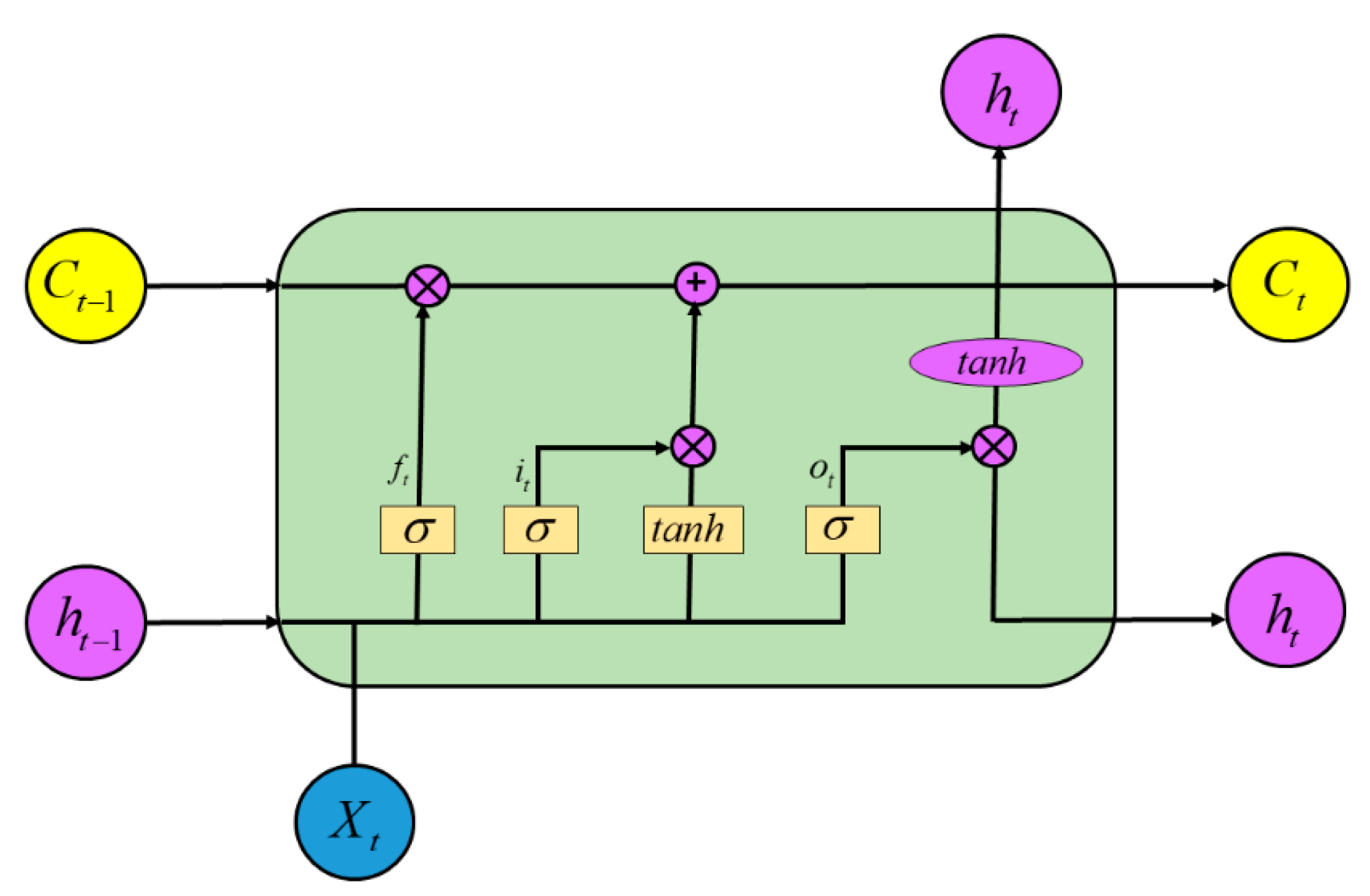
2.1. Long Short-Term Memory

Since 2006, deep learning [8] was proposed by Geoffrey Hinton, due to its lower cost, better robustness, and other advantages, which has been used in a wide range of research, including but not limited to image recognition [9], traffic flow prediction [10], stock market prediction [11], machine translation [12]. By adding the input gate, the forgetting gate and the output gate, LSTM can keep a long-term memory in time series [13]. In 2015, Chen et al. [14] used the LSTM model to predict the return rate of Chinese stocks. In 2021, Yan et al. [15] found that the multi-hour prediction based on the LSTM model was the optimal prediction model in the research on the prediction of a multi-station air quality index in Beijing. However, the LSTM model does not distinguish the importance of each time node information, and the introduction of an attention mechanism can better solve this problem [16]. In 2019, Chen et al. [17] used the LSTM model based on the attention mechanism to predict and discuss the trend of the Hong Kong stock market. The results show that after adding the attention mechanism, the positive and negative motion accuracy are improved by 3.06% and 0.26%, respectively, which proves that the LSTM model based on the attention mechanism has better performance than the original model. In 2021, Zheng et al. [18] added the attention mechanism to calculate different weights in the short-term traffic flow prediction to distinguish the importance of different time flow sequences. Hence, the prediction performance has been improved effectively.

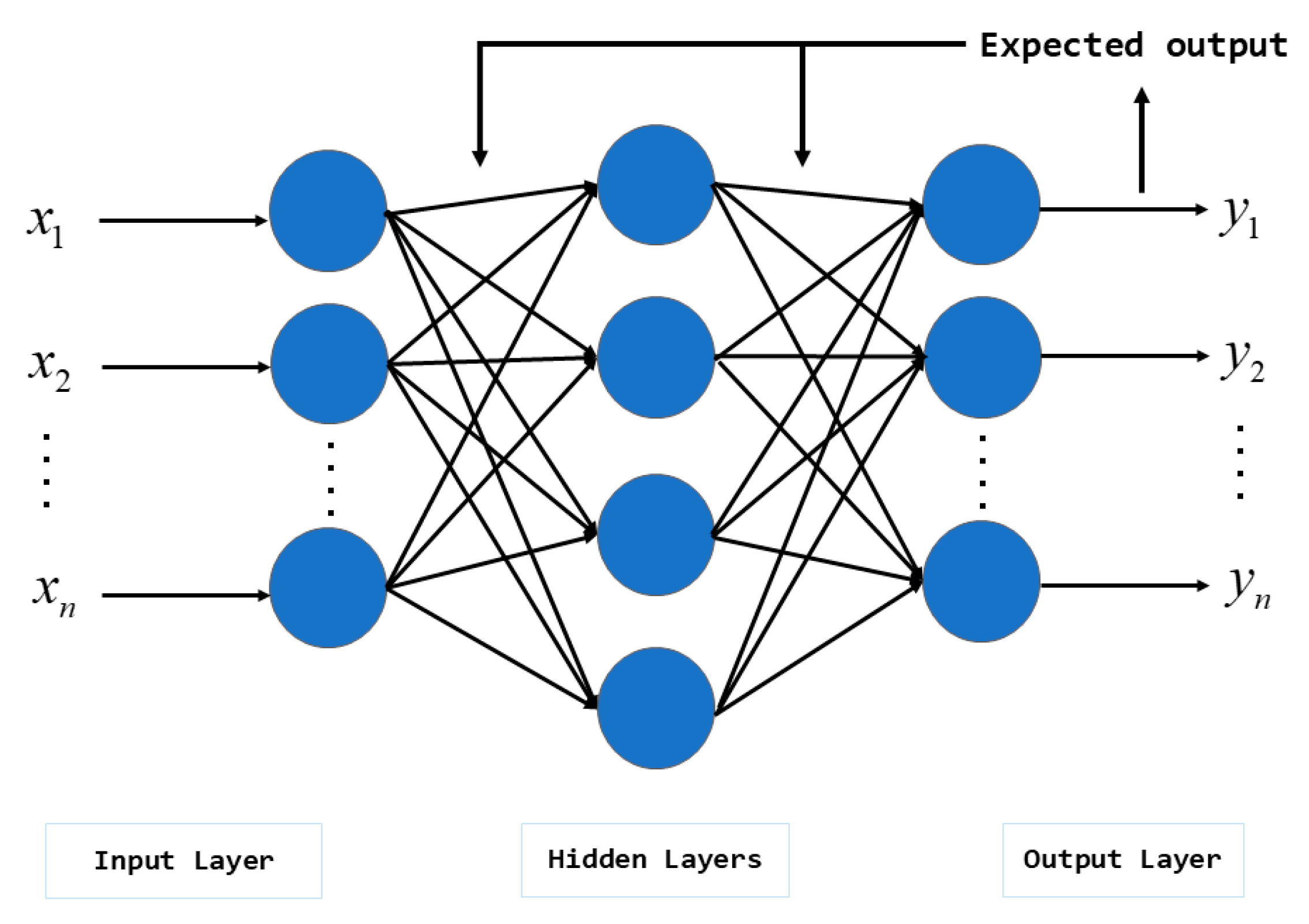
2.2. Back Propagation Neural Network

BP is a nonlinear multilayer feedforward neural network [19]. Because of its simple structure, outstanding performance of nonlinear mapping ability, and low computational complexity, this model is widely used in image processing, system simulation, optimal prediction, and other fields [20]. The theory and application to BP are relatively mature nowadays. In 2018, Li et al. [21] proposed an air pollution prediction model based on BPNN. In 2019, Hua et al. [22] proposed a short-term power prediction method for photovoltaic power plants based on the LSTM-BP model, and the experimental results show that the improved method has less prediction error. In 2022, Liu et al. [23] greatly improved the timeliness of prediction results through BPNN analyzing internet financial risks.

2.3. Autoregressive Integrated Moving Average

ARIMA, a famous and mature linear statistical model proposed by Box and Jenkins in the 1970s, can predict the future value by analyzing the relationship between the past time series [24]. This model, which is developed from the initial autoregressive (AR) model and the moving average (MA) model, has been successfully applied in many fields, such as oil production prediction, energy consumption prediction, and precipitation prediction [25]. In 2016, Sen et al. [26] revealed that ARIMA is the best prediction model in the experiment of predicting greenhouse gas emissions. In 2018, Oliveira et al. [27] used bootstrap aggregation and the ARIMA model to predict mid- and long-term power consumption. In 2019, Aasim et al. [28] proposed Repeated Wavelet Transform based on the ARIMA model for short-term wind speed prediction. In 2020, Lai et al. [29] used the statistical prediction model based on ARIMA to obtain the prediction results of local recent regional temperature and precipitation. In 2021, Fan et al. [30] used the ARIMA model and the LSTM model to predict oil well production. These studies show that ARIMA stands out with its relative stability in prediction.

2.4. The Association Rule Mining Algorithm

The association rule mining algorithm was first proposed by Agrawal et al. [31] in 1993. The downward closure feature is at the core of the apriori algorithm [32]. In order to solve the problem of the apriori algorithm generating a large number of candidate sets, Han et al. [33] introduced Frequent Pattern Tree Growth (FP-Tree Growth algorithm) in 2000. In 2001, H-mine proposed by Pei et al. [34] explored the super structure mining of frequent patterns to build alternative trees. In order to solve the problem of generating unnecessary candidate spanning trees during dynamic association rule mining, Xu et al. [35] proposed the IFP-Growth algorithm in 2002. In 2003, Liu et al. [36] proposed the condensed frequent pattern tree to elaborate on the principle of top-down and bottom-up traversal modes. Given that the importance varies across different transactions in actual data, in 2020, Shao et al. [37] proposed a mining algorithm prediction model based on correlation weighting. Wu et al. [38] proposed a frequent fuzzy item set mining method, which significantly increased the efficiency of the traditional apriori algorithm.

3. Data

3.1. Data Sources

Including futures prices in the prediction model is conducive to improving the accuracy of cash price prediction [39], and the current prices are vulnerable to different temporal and spatial factors. Therefore, in the study of corn price in Sichuan Province, we consider using futures prices and spot prices in the model. The experimental data are collected from China’s agricultural big data website, Dalian Commodity Exchange, and Zhengzhou Commodity Exchange. Various factors heavily struck the economy [40] and caused a rocketing price of agricultural products. In order to make an in-depth study of the situation when prices fluctuate violently, all the daily average price data were selected from March 2011 to April 2021. From China’s agricultural big data website, we collected the corn price data of some provinces in China, and the national average price data of corn, early rice, and middle-late rice. The soybean futures price data are collected from Dalian Commodity Exchange. Moreover, the futures price data of common wheat and high-quality strong gluten wheat are collected from Zhengzhou Commodity Exchange.

3.2. Data Cleaning

Due to the influence of holidays, some daily price data were missing. Moreover, some daily price data remained unchanged for several consecutive days, which hurt the experiment. To solve these two problems mentioned above, we converted the daily average price data into the weekly average price data. The data were numbered and sorted in time order, and finally 511 observations were obtained. Through the half violin plot, the data of agricultural products and future prices are displayed in Figure 2. Among them, China is the corn price in China; GD is the corn price in Guangdong; JL is the corn price in Jilin; LN is the corn price in Liaoning; JS is the corn price in Jiangsu; SD is the corn price in Shandong; ER is the early rice price; MLR is the middle-late rice price; WH is the high-quality strong gluten wheat futures price; PM is the common wheat futures price; Soybean is the soybeans futures price; and SC is the corn price in Sichuan.

3.3. Data Processing

Before the experiment, the values of the sample data need to be normalized. The normalization formula is as follows:
x * = x m i n m a x m i n
where m a x is the maximum value of data and m i n is the minimum value of data.
To understand whether the past price impacts the current price, we need to expand all price data forward by 12 horizons, that is three months, and make records in turn. Different agricultural products have different degrees of price change, so we must set different coefficients to judge the price change. By calculating the difference between the price of the previous 1 week, the previous 2 weeks to the previous 12 weeks, and the current week, comparing the difference with the set coefficient, the changes in the relationship between whether the price data are rising, falling, or remaining unchanged will be achieved (specific parameters are shown in Table 1). Then, according to the changing relationship in the price, by using the apriori algorithm, 12 spatial-temporal factors affecting the change of corn price in Sichuan Province are found, and there are 499 observations in each spatial-temporal factor.
In the apriori algorithm, the degree of support is generally expressed as P ( A B ) , which represents the probability of simultaneous occurrence of item sets A and B in transaction T , the specific formula is:
s u p p o r t ( A B ) = P ( A B ) = c o u n t ( A B ) c o u n t ( T )
The confidence is generally expressed as P ( B | A ) , which represents the percentage of dataset B contained in dataset A , that is the conditional probability of occurrence of B under the condition that A occurs. The specific formula is:
c o n f i d e n c e ( A B ) = P ( B | A ) = c o u n t ( A B ) c o u n t ( A )
By utilizing the method of training test segmentation, the data obtained by the apriori algorithm is divided into training sets and test sets in the radio of eight to two. The prediction results are obtained by putting the data into the forecast model for training.

3.4. Performance Index

In the study of corn prices in Sichuan Province, we use root mean square error (RMSE), mean absolute percentage error (MAPE), and mean absolute error (MAE) to calculate the prediction errors of each model. The fitting degree between the predicted value and the actual value is judged by calculating the value of the determined coefficient R 2 . The calculation formulas of RMSE, MAPE, MAE, and determination coefficient R 2 are as follows:
RMSE = 1 N t = 1 N ( y t y ^ t )
MAPE = 1 N t = 1 N | y t y ^ t | y t
MAE = 1 N t = 1 N | y t y ^ t |
R 2 = ( y ^ t y ¯ t ) 2 ( y t y ¯ t ) 2
where y t represents the real value; y ^ t represents the predicted value; y ¯ t represents the average value of the real value; and N represents the total number of data.

4. Materials and Methods

4.1. Linear Regression Model

The linear regression (LR) model is one of the most widely used models in the field of prediction. It is necessary to observe the dependent variable Y and p predictors, and the independent variable X 1 , X 2 , , X p , respectively, to construct the linear relationship between the two variables. The specific formula is [41]:
Y = β 0 + β 1 X 1 + + β p X p + ε .
where β 0 , β 1 , , β p represent the regression coefficient of each influencing independent variable, and ε represents the random disturbance or error, which is assumed to follow the normal distribution with a mean of zero and a constant variance.

4.2. Random Forest Model

Random Forest (RF) model is the representative of the Bagging algorithm in ensemble learning [42]. In RF, the correlation between trees is reduced by randomization in both directions [43]. The random forest will first select N samples randomly from all the sample sets, and then select K features randomly from the feature values. In the selected samples, an optimal partition feature is selected to establish a decision tree. The above two steps are repeated M times, that is, M decision trees are generated to form a random forest. Therefore, the Random Forest model is a prediction model composed of multiple decision trees, which can integrate some weak learners into strong learners.

4.3. Extreme Gradient Boosting Model

The XGBoost model is a supervised machine learning algorithm based on Pre-Ordering. The concept of it is to sequence all the feature data according to their numerical value, search for the best segmentation point, achieve the effect of reducing forecast error, and finally improve its accuracy after splitting the data into left and right nodes [44]. Therefore, the XGBoost model is a representative of the Boosting algorithm in ensemble learning [45], which can accurately capture the nonlinear characteristics between various predictive variables.

4.4. Light Gradient Boosting Machine Model

The LightGBM model is a relatively novel and efficient gradient lifting decision tree algorithm, which can solve the problems of excessive space consumption in the XGBoost model [46]. By using the Gradient-based One-Side Sampling (GOSS) technology to reduce the data with small gradient, the LightGBM model can save space-time expenses. Moreover, by utilizing the Exclusive Feature Bundling (EFB) technology to bind mutually exclusive features into one, this model can reduce dimensions. [47]. Therefore, compared with the traditional Gradient Boosting Decision Tree (GBDT) model, the LightGBM model has the characteristics of faster training speed and rapid processing of massive data [48].

4.5. LSTM Model

LSTM is a neural network model that processes time series. It can predict not only univariate time series, but also multivariate time series data [49]. The model structure is shown in Figure 3.
Among them, “gate” is the key technology of the LSTM model. By controlling the input, storage, and output of the data, LSTM can deal with the problems such as long-term dependence and gradient explosion [50]. The detailed formula is given by the following equation:
f t = σ ( W f [ h t 1 , x t ] + b f )
i t = σ ( W i [ h t 1 , x t ] + b i )
o t = σ ( W o [ h t 1 , x t ] + b o )
C t = f t C t 1 + i t ( W c [ h t 1 , x t ] + b g )
h t = o t tanh ( C t )
where W f , W i , W o , W c are weight matrix; b f , b i , b o , b g are offset vectors; σ is the sigmoid activation function; f t is the forgetting gate; i t is the input gate; o t is the output gate; C t is the cell state and h t is the unit output.

4.6. AttLSTM Model

The AttLSTM model combines the LSTM model and attention mechanism [51], and the model structure is shown in Figure 4. From Figure 4, we can see that the AttLSTM model has four parts, namely the input layer, the LSTM layer, the attention layer, and the output layer. In decoding, the attention mechanism uses the scoring function to calculate the weights of different inputs, which changes the traditional encode-decode structure [52]. The input vectors of the layer enter the LSTM units in the LSTM layer, and become the h 1 , h 2 , , h t vectors. After nonlinear transformation, the u 1 , u 2 , , u t vectors are generated. The specific formula is as follows:
u t = tanh ( W t h t + b t )
where W t is the weight coefficient and b t is the offset vector. After the vectors enter the attention layer from the LSTM layer, after normalization and the weighted-sum approach, the feature representation V is generated. The specific formula is as follows:
α t = exp ( u t T u s ) t = 1 t exp ( u t T u s )
V = t = 1 t α t h t
where u s represents the initialized random attention matrix. Finally, the data vectors are transferred to the output layer for training, and the results are obtained.

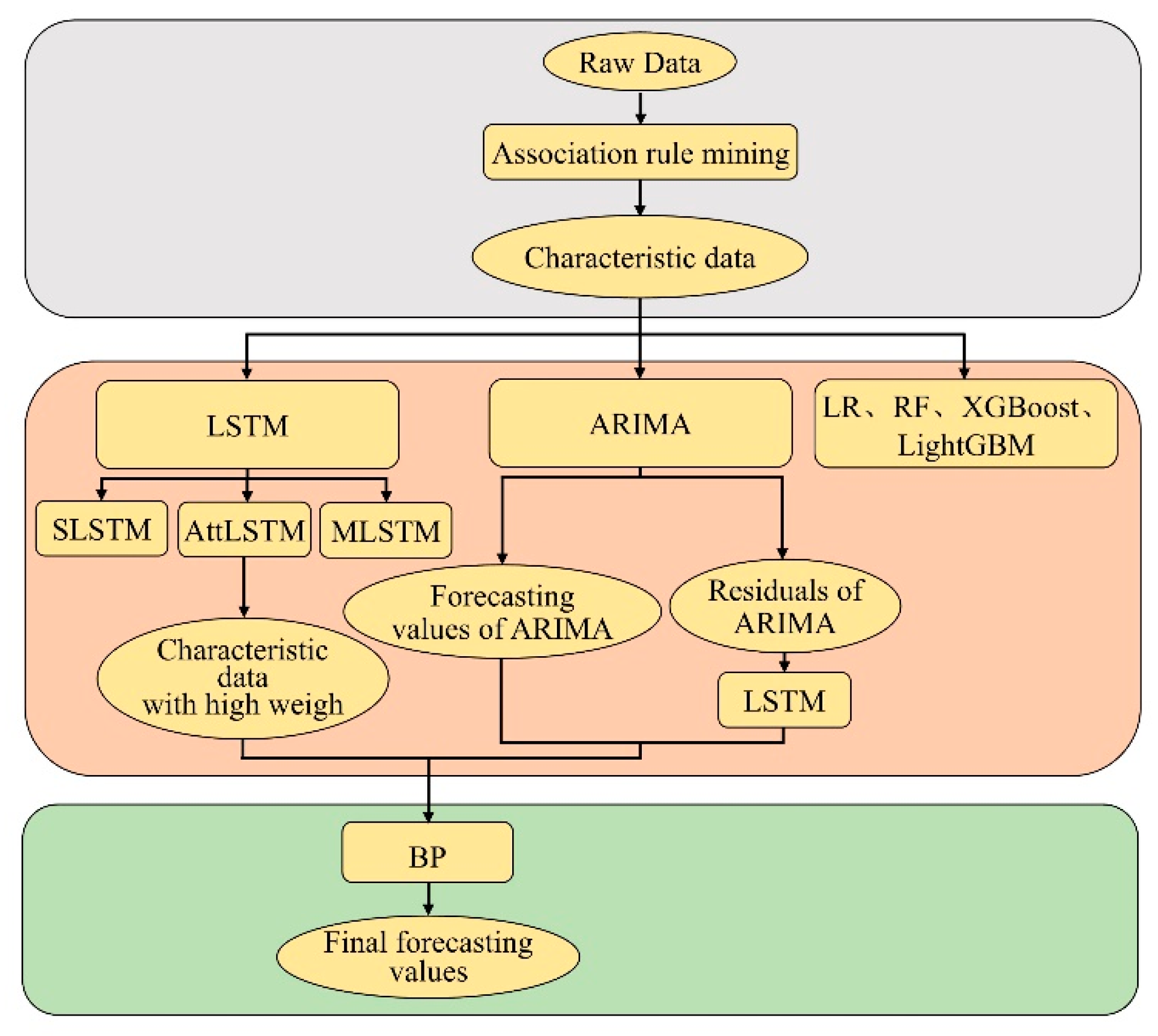
4.7. AttLSTM-ARIMA-BP Combination Model

In this paper, we propose a combined model of AttLSTM-ARIMA-BP to study the corn price data in Sichuan Province.
ARIMA is a simple prediction model, without the help of other variables, which can predict a single column of data by using the correlation between time series [53]. The specific formula is as follows:
( 1 i = 1 p ϕ i L i ) ( 1 L ) d X t = ( 1 + i = 1 q ϕ i L i ) ε t
where L is the lag operator; p is the autoregressive order; d is the number of differences; q is the moving average order; and ε t is the white noise.
However, ARIMA can only predict the linear relationship between the corn price data. The farther the target is from the historical data, the worse the prediction is [54]. Therefore, we consider using a combination model to solve this problem.
In the combination algorithm of the traditional ARIMA model, the residual data obtained from ARIMA is trained by LSTM, the trained result is regarded as linear. The linear addition method is used to add the results trained by LSTM, and the prediction results obtained by ARIMA, to predict the final results [55]. The specific formula is as follows:
y t = m t + n t
r t = y t m t ^
y t ^ = m t ^ + r t ^
where y t is the raw data; m t is the linear part of the raw data; n t is the nonlinear part of the raw data; r t is the residual data obtained by ARIMA; m t ^ is the predicted data obtained by ARIMA training m t ; r t ^ is the training results obtained by LSTM training r t ; and y t ^ is the final prediction result.
Sometimes, mere linear addition cannot improve the accuracy of the final prediction, because the relationship between the prediction results of LSTM and ARIMA may be nonlinear [56]. Therefore, we consider using the BP model to train the prediction results of LSTM and ARIMA. The specific formula is as follows:
y t ^ = f ( m t ^ , r t ^ )
The core of the BP neural network model is an error analysis according to training results and expected effect, and the expected results are finally obtained by modifying weights and thresholds [57]. The specific formula is as follows:
y i = f ( i = 1 m w i x i )
where w i is the prominence weight; x i is the Input signa; f is the Activate function; and y i is the output result. The model structure is shown in Figure 5.
Since the final prediction effect of the model will be affected by other factors, we select several groups of data with the highest weight as the input of the model through the attention mechanism. Through the BP model training the predicted value m t ^ obtained by ARIMA, the residual value r t ^ obtained by LSTM, and several groups of data with the highest weight a t selected by the attention mechanism, the predicted results are finally obtained. The specific formula is as follows:
y t ^ = f ( m t ^ , r t ^ , a t )
The specific implementation process of the model is as follows:
Step 1.
Input the raw data of corn price in the ARIMA model to obtain the predicted value m t ^ and the residual value r t .
Step 2.
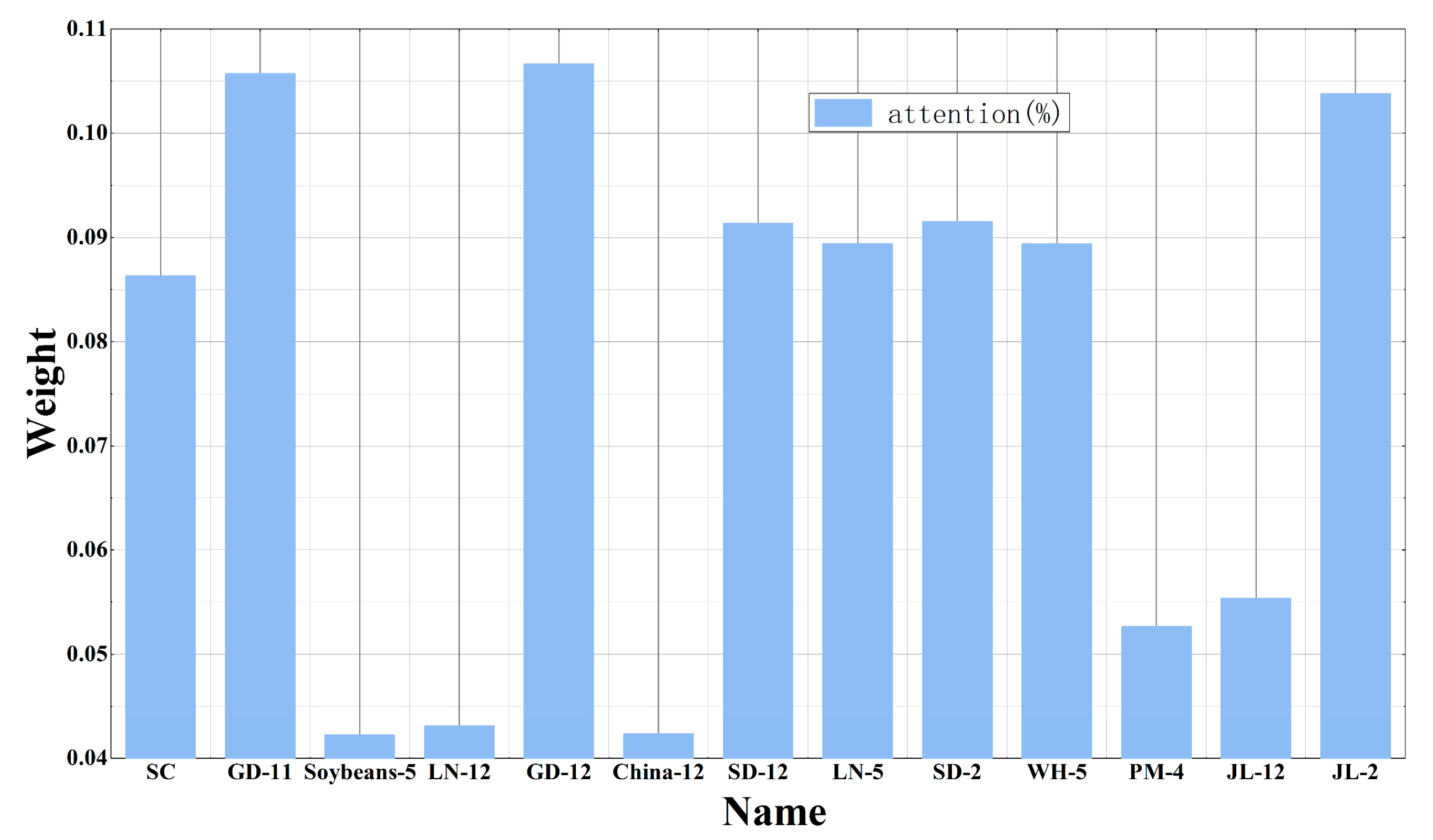
Use the attention mechanism to calculate the weight of corn price data in Sichuan Province, and select the data with the top three weight influencing factors a t as the input of the subsequent model.
Step 3.
Train the residual data r t by LSTM and obtain the training value r t ^ .
Step 4.
Obtain the final predicted value by inputting the m t ^ , r t ^ , and a t to the BP.

4.8. Experimental Design

In the research of corn price forecast in Sichuan Province, we used the LR model and the ARIMA model in statistics; RF, XGBoost, LightGBM, LSTM, AttLSTM, and BP models in machine learning. Among them, the ARIMA model was completed by Eviews, LR, RF, XGBoost, and LightGBM models were implemented by the Scikit-learn package. We used Keras in Python to run LSTM and AttLSTM models. In addition, under this environment, we combined AttLSTM, ARIMA, and BP models into the AttLSTM-BP-ARIMA model to study the corn price in Sichuan Province. The parameter settings of each model are shown in Table 2.

5. Results and Discussion

5.1. The Results of the Predictive Regression Models

In the predictive regression model, we respectively use LR, RF, XGBoost, and LightGBM models to study corn prices in Sichuan Province, where RF, XGBoost, and LightGBM models are predictive regression models in ensemble learning [58]. The experimental results are shown in Figure 6a, where the red, blue, green, and purple dots represent the predicted values of the LR, RF, LightGBM, and XGBoost models, respectively.
Firstly, we can observe from Figure 6a that the predicted values of the first 88 ensemble learning models are consistent with the changing trend and fluctuation of the real values, but from the 88th data, the real values and predicted values vary greatly. In LR, the experimental results of the latter part are better than the ensemble learning model mentioned above. However, there is still a defect that the prediction effect of some intervals is not ideal, such as the 55th to 72th, and the last four intervals.
Secondly, divide the prediction results of the predictive regression model into five parts, each of which has 20 groups of data. Calculate the MAE value of each par, respectively, and sort the error value into Table 3. We can observe from Table 3 that in ensemble learning, the last part of the data has the largest error value. In LR, although the predictive error value of the last part of the data is relatively small, the number itself is still large, and the largest error value is the second and the third part of the data. To sum up, in the case of bouncing fluctuations in corn prices in Sichuan Province, the prediction accuracy of the predictive regression model is not ideal.

5.2. The Results of LSTM Models

Regarding the problem of the predictive regression model having an unsatisfying result when the price of corn fluctuates by leaps and bounds, we adopted LSTM to study the price data further.
Through the single LSTM model, we conclude that the prediction accuracy will reach its peak when predicting next week’s price based on the corn price data of Sichuan Province over the past four weeks. To compare the prediction accuracy of each LSTM model more conveniently, we set the time window of all LSTM models to 4, so a total of 99 price data are predicted. It can be seen from the orange line in Figure 6b that although the single LSTM model can well predict the changing trend and fluctuation of the price, the prediction result still has the hysteresis quality. Hence, the single LSTM model is not desirable.
To solve the problem of hysteresis quality, we adopted a multivariate LSTM model to predict the price of corn in Sichuan Province. It can be seen from the blue line in Figure 6b that although the multivariate LSTM model solves the problem of hysteresis quality, its image looks like a “smooth” curve, and hence we cannot predict the fluctuation of price changes. So, the multivariate LSTM model is also not desirable.
The attention mechanism performs well when capturing price fluctuations [59], so we continue to research corn prices in Sichuan Province by integrating the attention mechanism into LSTM. The weight of each column’s value in agricultural and futures prices are shown in Figure 7. As observed from the pink line in Figure 6b, in terms of price change trends and price fluctuations, AttLSTM can do a good job of predicting the price of corn in Sichuan Province. To illustrate the prediction accuracy of AttLSTM more rationally, we collated the resultant errors of each LSTM model into Table 4. Compared with the predictive regression model, only the AttLSTM model, especially the first four data sets, has shown a significant improvement in the accuracy of prediction. For the last data set, the AttLSTM model still failed to achieve the desired prediction.

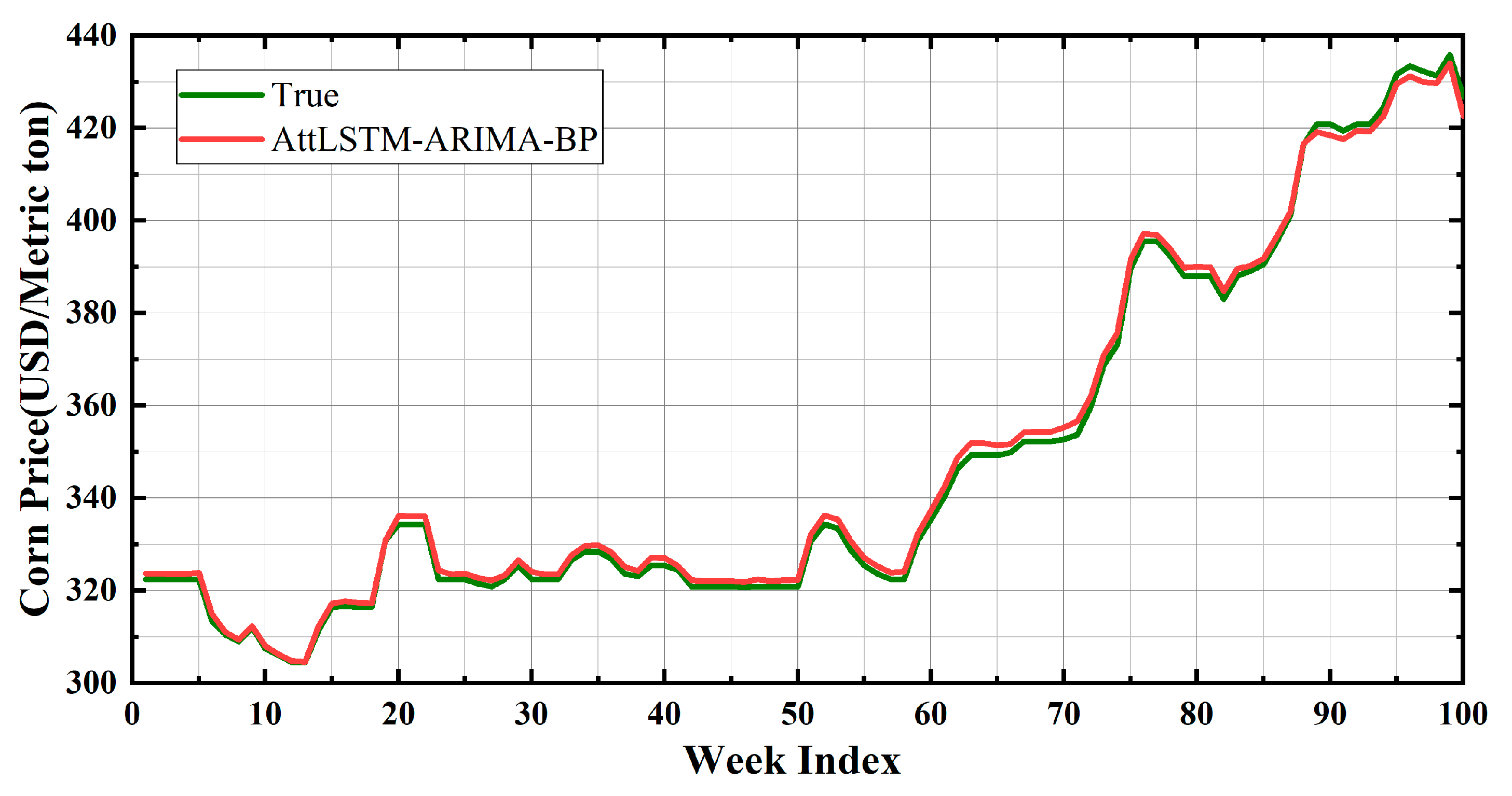
5.3. The Prediction Result of the AttLSTM-ARIMA-BP Model

Given that the ARIMA model can only predict linear relationships in prices, and the further the target is from the historical data, the worse the prediction is. To completely solve the problem of hysteresis quality, we input the predicted values obtained from the ARIMA model and the residuals obtained from the LSTM model in the BP model. Since the past price always affects the current price, we also select the three columns with the maximum weights in Figure 7 to research the corn price in Sichuan Province, namely the price of corn in Guangdong Province 12 weeks ago, the price of corn in Guangdong Province 11 weeks ago, and the price of corn in Jilin Province 2 weeks ago. Through the BP model training the predicted value obtained by ARIMA, the residual value obtained by LSTM training, and the three sets of data with the highest weight obtained by the attention mechanism, the price of corn in Sichuan Province is predicted. We divide the prediction results of the model into five parts, each of which has 20 groups of data. Then, we calculate the MAE value of each par, respectively, and sort the error value into Table 4. By judging the fitting degree in Figure 8 and analyzing the MAE score in Table 4, we conclude that the AttLSTM-ARIMA-BP model can accurately predict the corn price in Sichuan Province, whether the price changes steadily or the price fluctuates by leaps and bounds.

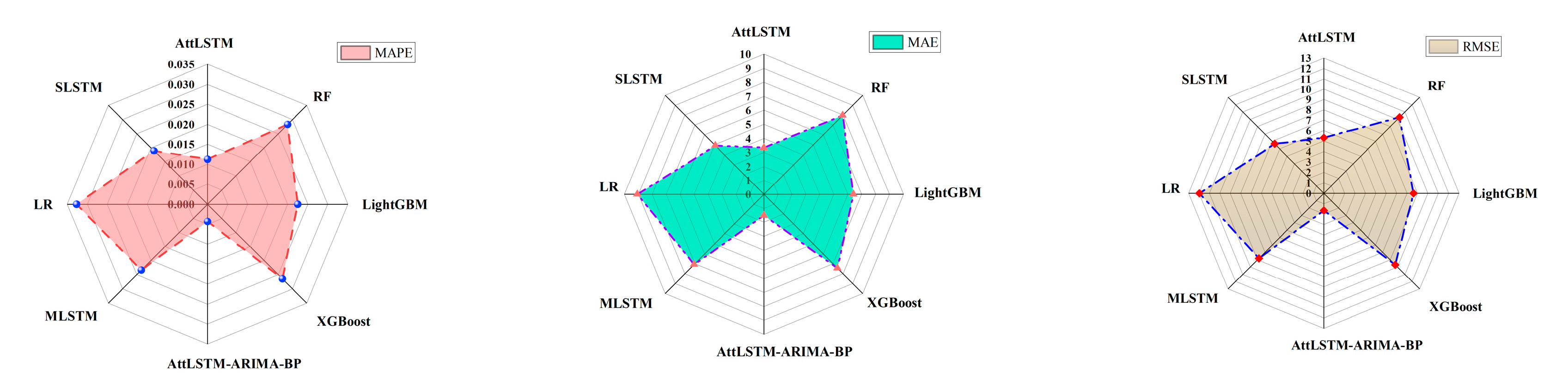
5.4. Experimental Comparison

In this part, by comparing the MAPE, RMSE, MAE, and R 2 of each model, the prediction effect of each model is analyzed.
As can be seen in Figure 9, no matter which error calculation method that we adopted, the AttLSTM-ARIMA-BP model recorded the smallest error value, where the MAPE was 0.0043, the MAE was 1.51, and the RMSE was 1.642, whereas the ensemble learning recorded the largest error value. In Figure 10, we set the horizontal coordinates to the true value of corn prices in Sichuan Province and the vertical coordinates to the predicted value, fitted the curve from the scatter plot, and calculated the value of the coefficient of determination R 2 . By comparison, the AttLSTM-ARIMA-BP model has the highest R 2 , which is 0.9992.

5.5. Experimental Discussion

Because of some uncontrollable factors, agricultural prices fluctuate dramatically, and traditional forecasting models can achieve good forecasts when prices change smoothly. When prices fluctuate dramatically, the models fail to achieve the ideal forecasting results.
Among the predictive regression models, RF, LightGBM, and XGBoost models can only show high accuracy when prices are changing mildly, whereas the LR model can give precise predictions when prices are just started to bounce. In the single LSTM model, the problem of hysteresis quality will appear in the prediction results. AttLSTM can improve the accuracy of the prediction results, but the prediction result is still not perfect when the price bounces. Because of the smallest error values and the largest R 2 , the AttLSTM-ARIMA-BP model can accurately predict the price of corn in Sichuan Province whether the price is a steady change or a dramatic fluctuation. Moreover, this model will have a broader application and development prospect in the research of time series data.

6. Conclusions

The price of agricultural products is the key element in agricultural sustainable development, which has a strong interaction with the economy. In recent years, the large-scale fluctuations in national food prices have been frequent, which have had a significant impact on society. This paper applies the apriori algorithm to study agricultural product prices in different regions and futures prices. The conclusion that prices in different times and spaces affect current prices is reached. Through several experiments, a combined AttLSTM-ARIMA-BP price forecasting model is finally proposed. This model is not only suitable for price forecasting in periods of steady data changes, but also gives accurate forecasts in times of great price changes. The results of this study are helpful for economists to formulate hedging strategies in the face of the market’s self-regulation drawbacks, and for investors to make the best asset allocation decisions, thus reducing risks in all aspects. In addition, this study enriches the existing theory of price forecasting models and contributes to the sustainable development of the agricultural products market.
To improve the accuracy of the model’s prediction results, we should also take the influence of international local war conflicts, epidemic situation, transportation, storage, and natural disasters into account. In the era of big data, people’s worries about the market on the internet can also lead to huge price fluctuations. In the follow-up study, the robustness and practicability of the model can be improved by collecting more data and adding perturbation factors to the model. We believe that the forecasting model proposed in this paper can make accurate predictions in times of dramatic price fluctuations, thus making an important contribution to market regulation and the sustainable economic development.

Author Contributions

Conceptualization, Y.G.; methodology, F.Z. and D.T.; software, D.T. and W.T.; validation, Y.F. and Q.T.; formal analysis, Y.G.; investigation, S.Y.; resources, Y.G.; data curation, S.Y.; writing—original draft preparation, F.Z. and D.T.; writing—review and editing, W.T., Y.F. and Q.T.; visualization, D.T.; supervision, F.Z.; project administration, Y.G.; funding acquisition, F.Z. All authors have read and agreed to the published version of the manuscript.

Funding

This research was funded by the Key Laboratory of Agriculture Information Engineering of Sichuan Province and Social Science Foundation of Sichuan Province in 2019 (SC19C032) and the Key Areas and Research Directions of Innovative Development of Digital Agriculture in Sichuan Province (2020PTYB16).

Institutional Review Board Statement

Not applicable.

Informed Consent Statement

Not applicable.

Data Availability Statement

The data used in the research of this paper comes from the website: http://www.agdata.cn/dataManual/dataIndustryTree (accessed on 10 May 2021), http://www.czce.com.cn/cn/sspz/H7702index_1.htm (accessed on 5 March 2022) and http://www.dce.com.cn/dalianshangpin/sspz/487124/index.html (accessed on 5 March 2022).

Acknowledgments

Thanks for the help of the Key Laboratory of Agriculture Information Engineering of Sichuan Province and Social Science Foundation of Sichuan Province and the Key Areas and Research Directions of Innovative Development of Digital Agriculture in Sichuan Province.

Conflicts of Interest

The authors declare no conflict of interest. The funders had no role in the design of the study; in the collection, analyses, or interpretation of data; in the writing of the manuscript; or in the decision to publish the results.

References

  1. Abdallah, M.B.; Farkas, M.F.; Lakner, Z. Analysis of meat price volatility and volatility spillovers in Finland. Agric. Econ. 2020, 66, 84–91. [Google Scholar] [CrossRef]
  2. Drachal, K. Some novel Bayesian model combination schemes: An application to commodities prices. Sustainability 2018, 10, 2801. [Google Scholar] [CrossRef] [Green Version]
  3. Cohen, G. Forecasting Bitcoin trends using algorithmic learning systems. Entropy 2020, 22, 838. [Google Scholar] [CrossRef] [PubMed]
  4. Verteramo Chiu, L.J.; Tomek, W.G. Insights from Anticipatory Prices. J. Agric. Econ. 2018, 69, 351–364. [Google Scholar] [CrossRef] [Green Version]
  5. Zheng, H.; Yuan, J.; Chen, L. Short-term load forecasting using EMD-LSTM neural networks with a Xgboost algorithm for feature importance evaluation. Energies 2017, 10, 1168. [Google Scholar] [CrossRef] [Green Version]
  6. Niu, M.; Hu, Y.; Sun, S.; Liu, Y. A novel hybrid decomposition-ensemble model based on VMD and HGWO for container throughput forecasting. Appl. Math. Model. 2018, 57, 163–178. [Google Scholar] [CrossRef]
  7. Guo, Y.; Hu, X.; Wang, Z.; Tang, W.; Liu, D.; Luo, Y.; Xu, H. The butterfly effect in the price of agricultural products: A multidimensional spatial-temporal association mining. Agric. Econ. 2021, 67, 457–467. [Google Scholar] [CrossRef]
  8. LeCun, Y.; Bengio, Y.; Hinton, G. Deep learning. Nature 2015, 521, 436–444. [Google Scholar] [CrossRef]
  9. Rajan, S.; Chenniappan, P.; Devaraj, S.; Madian, N. Novel deep learning model for facial expression recognition based on maximum boosted CNN and LSTM. IET Image Process. 2020, 14, 1373–1381. [Google Scholar] [CrossRef]
  10. Zheng, J.; Huang, M. Traffic flow forecast through time series analysis based on deep learning. IEEE Access 2020, 8, 82562–82570. [Google Scholar] [CrossRef]
  11. Ji, Y.; Liew, A.W.C.; Yang, L. A novel improved particle swarm optimization with long-short term memory hybrid model for stock indices forecast. IEEE Access 2021, 9, 23660–23671. [Google Scholar] [CrossRef]
  12. Jian, L.; Xiang, H.; Le, G. LSTM-Based Attentional Embedding for English Machine Translation. Sci. Program. 2022, 2022, 3909726. [Google Scholar] [CrossRef]
  13. Hochreiter, S.; Schmidhuber, J. Long short-term memory. Neural Comput. 1997, 9, 1735–1780. [Google Scholar] [CrossRef]
  14. Chen, K.; Zhou, Y.; Dai, F. A LSTM-based method for stock returns prediction: A case study of China stock market. In Proceedings of the 2015 IEEE International Conference on Big Data, Santa Clara, CA, USA, 29 October 2015–1 November 2015; pp. 2823–2824. [Google Scholar]
  15. Yan, R.; Liao, J.; Yang, J.; Sun, W.; Nong, M.; Li, F. Multi-hour and multi-site air quality index forecasting in Beijing using CNN, LSTM, CNN-LSTM, and spatiotemporal clustering. Expert Syst. Appl. 2021, 169, 114513. [Google Scholar] [CrossRef]
  16. Bahdanau, D.; Cho, K.; Bengio, Y. Neural machine translation by jointly learning to align and translate. arXiv 2014, arXiv:1409.0473. [Google Scholar]
  17. Chen, S.; Ge, L. Exploring the attention mechanism in LSTM-based Hong Kong stock price movement prediction. Quant. Financ. 2019, 19, 1507–1515. [Google Scholar] [CrossRef]
  18. Zheng, H.; Lin, F.; Feng, X.; Chen, Y. A hybrid deep learning model with attention-based conv-LSTM networks for short-term traffic flow prediction. IEEE Trans. Intell. Transp. Syst. 2020, 22, 6910–6920. [Google Scholar] [CrossRef]
  19. Rumelhart, D.E.; Hinton, G.E.; Williams, R.J. Learning representations by back-propagating errors. Nature 1986, 323, 533–536. [Google Scholar] [CrossRef]
  20. Hu, H.; Tang, L.; Zhang, S.; Wang, H. Predicting the direction of stock markets using optimized neural networks with Google Trends. Neurocomputing 2018, 285, 188–195. [Google Scholar] [CrossRef]
  21. Li, A.; Xu, X. A new pm2. 5 air pollution forecasting model based on data mining and bp neural network model. In Proceedings of the 2018 3rd International Conference on Communications, Information Management and Network Security (CIMNS 2018), Wuhan, China, 27–28 September 2018; pp. 110–113. [Google Scholar]
  22. Hua, C.; Zhu, E.; Kuang, L.; Pi, D. Short-term power prediction of photovoltaic power station based on long short-term memory-back-propagation. Int. J. Distrib. Sens. Netw. 2019, 15, 3134. [Google Scholar] [CrossRef]
  23. Liu, Z.; Du, G.; Zhou, S.; Lu, H.; Ji, H. Analysis of internet financial risks based on deep learning and BP neural network. Comput. Econ. 2022, 59, 1481–1499. [Google Scholar] [CrossRef]
  24. Box, G.E.P.; Jenkins, G.M.; Reinsel, G.C.; Ljung, G.M. Time Series Analysis: Forecasting and Control, 5th ed.; Wiley: Hoboken, NJ, USA, 2015. [Google Scholar]
  25. Suganthi, L.; Samuel, A.A. Modelling and forecasting energy consumption in INDIA: Influence of socioeconomic variables. Energy Source Part B 2016, 11, 404–411. [Google Scholar] [CrossRef]
  26. Sen, P.; Roy, M.; Pal, P. Application of ARIMA for forecasting energy consumption and GHG emission: A case study of an Indian pig iron manufacturing organization. Energy 2016, 116, 1031–1038. [Google Scholar] [CrossRef]
  27. De Oliveira, E.M.; Oliveira, F.L.C. Forecasting mid-long term electric energy consumption through bagging ARIMA and exponential smoothing methods. Energy 2018, 144, 776–788. [Google Scholar] [CrossRef]
  28. Singh, S.N.; Mohapatra, A. Repeated wavelet transform based ARIMA model for very short-term wind speed forecasting. Renew. Energy 2019, 136, 758–768. [Google Scholar]
  29. Lai, Y.; Dzombak, D.A. Use of the autoregressive integrated moving average (ARIMA) model to forecast near-term regional temperature and precipitation. Weather Forecast. 2020, 35, 959–976. [Google Scholar] [CrossRef]
  30. Fan, D.; Sun, H.; Yao, J.; Zhang, K.; Yan, X.; Sun, Z. Well production forecasting based on ARIMA-LSTM model considering manual operations. Energy 2021, 220, 119708. [Google Scholar] [CrossRef]
  31. Agrawal, R.; Imieliński, T.; Swami, A. Mining association rules between sets of items in large databases. In Proceedings of the 1993 ACM SIGMOD International Conference on Management of Data, Washington, DC, USA, 25–28 May 1993; Volume 22, pp. 207–216. [Google Scholar]
  32. Agrawal, R.; Srikant, R. Fast algorithms for mining association rules. In Proceedings of the 20th International Conference on Very Large Data Bases, Santiago de Chile, Chile, 12 September 1994; pp. 487–499. [Google Scholar]
  33. Han, J.; Pei, J.; Yin, Y.; Mao, R. Mining frequent patterns without candidate generation: A frequent-pattern tree approach. Data Min. Knowl. Discov. 2004, 8, 53–87. [Google Scholar] [CrossRef]
  34. Pei, J.; Han, J.; Mortazavi-Asl, B.; Pinto, H.; Chen, Q.; Dayal, U.; Hsu, M. Mining sequential patterns efficiently by prefix-projected pattern growth. In Proceedings of the 17th International Conference on Data Engineering, Heidelberg, Germany, 2–6 April 2001. [Google Scholar]
  35. Xu, B.; Yi, T.; Wu, F.; Chen, Z. An incremental updating algorithm for mining association rules. J. Electron. 2002, 19, 403–407. [Google Scholar] [CrossRef]
  36. Liu, G.; Lu, H.; Lou, W.; Yu, J. On computing, storing and querying frequent patterns. In Proceedings of the Ninth ACM SIGKDD International Conference on Knowledge Discovery and Data Mining, Washington, DC, USA, 24–27 August 2003; pp. 607–612. [Google Scholar]
  37. Shao, Y.; Liu, B.; Wang, S.; Li, G. Software defect prediction based on correlation weighted class association rule mining. Knowl. Based Syst. 2020, 196, 105742. [Google Scholar] [CrossRef]
  38. Wu, T.Y.; Lin, J.C.W.; Yun, U.; Chen, C.; Srivastava, G.; Lv, X. An efficient algorithm for fuzzy frequent itemset mining. J. Intell. Fuzzy Syst. 2020, 38, 5787–5797. [Google Scholar] [CrossRef]
  39. Yang, J.; Bessler, D.A.; Leatham, D.J. Asset storability and price discovery in commodity futures markets: A new look. J. Futures Mark. 2001, 21, 279–300. [Google Scholar] [CrossRef]
  40. Sako, K.; Mpinda, B.N.; Rodrigues, P.C. Neural Networks for Financial Time Series Forecasting. Entropy 2022, 24, 657. [Google Scholar] [CrossRef] [PubMed]
  41. Paul, R.K.; Vennila, S.; Yeasin, M.; Yadav, S.K.; Nisar, S.; Paul, A.K.; Gupta, A.; Malathi, M.K.J.; Kavitha, Z.; Mathukumalli, S.R.; et al. Wavelet Decomposition and Machine Learning Technique for Predicting Occurrence of Spiders in Pigeon Pea. Agronomy 2022, 12, 1429. [Google Scholar] [CrossRef]
  42. Zhang, F.; Wen, N. Carbon price forecasting: A novel deep learning approach. Environ. Sci. Pollut. Res. 2022, 29, 54782–54795. [Google Scholar] [CrossRef]
  43. Paul, R.K.; Yeasin, M.; Kumar, P.; Kumar, P.; Balasubramanian, M.; Roy, H.S.; Roy, H.S.; Gupta, A.K. Machine learning techniques for forecasting agricultural prices: A case of brinjal in Odisha. PLoS ONE 2022, 17, e0270553. [Google Scholar] [CrossRef]
  44. Phan, Q.T.; Wu, Y.K.; Phan, Q.D. A hybrid wind power forecasting model with XGBoost, data preprocessing considering different NWPs. Appl. Sci. 2021, 11, 1100. [Google Scholar]
  45. Zhou, Y.; Li, T.; Shi, J.; Qian, Z. A CEEMDAN and XGBOOST-based approach to forecast crude oil prices. Complexity 2019, 2019, 4392785. [Google Scholar] [CrossRef] [Green Version]
  46. Jiang, M.; Liu, J.; Zhang, L.; Liu, C. An improved Stacking framework for stock index prediction by leveraging tree-based ensemble models and deep learning algorithms. Physica A 2020, 541, 122272. [Google Scholar] [CrossRef]
  47. Jabeur, S.B.; Mefteh-Wali, S.; Viviani, J.L. Forecasting gold price with the XGBoost algorithm and SHAP interaction values. Ann. Oper. Res. 2021, 1–21. [Google Scholar] [CrossRef]
  48. Sun, X.; Liu, M.; Sima, Z. A novel cryptocurrency price trend forecasting model based on LightGBM. Financ. Res. Lett. 2020, 32, 101084. [Google Scholar] [CrossRef]
  49. Liu, Y.; Yang, C.; Huang, K.; Gui, W. Non-ferrous metals price forecasting based on variational mode decomposition and LSTM network. Knowl. Based Syst. 2020, 188, 105006. [Google Scholar] [CrossRef]
  50. Kontogiannis, D.; Bargiotas, D.; Daskalopulu, A. Minutely active power forecasting models using neural networks. Sustainability 2020, 12, 3177. [Google Scholar] [CrossRef] [Green Version]
  51. Yin, H.; Jin, D.; Gu, Y.H.; Park, C.J.; Han, S.K.; Yoo, S.J. STL-ATTLSTM: Vegetable price forecasting using STL and attention mechanism-based LSTM. Agriculture 2020, 10, 612. [Google Scholar] [CrossRef]
  52. Zhang, Q.; Yang, L.; Zhou, F. Attention enhanced long short-term memory network with multi-source heterogeneous information fusion: An application to BGI Genomics. Inf. Sci. 2021, 553, 305–330. [Google Scholar] [CrossRef]
  53. Wang, J.; Li, X.; Hong, T.; Wang, S. A semi-heterogeneous approach to combining crude oil price forecasts. Inf. Sci. 2018, 460, 279–292. [Google Scholar] [CrossRef]
  54. Dou, Z.; Ji, M.; Wang, M.; Shao, Y. Price Prediction of Pu’er tea based on ARIMA and BP Models. Neural Comput. Appl. 2022, 34, 3495–3511. [Google Scholar] [CrossRef]
  55. Xu, D.; Zhang, Q.; Ding, Y.; Zhang, D. Application of a hybrid ARIMA-LSTM model based on the SPEI for drought forecasting. Environ. Sci. Pollut. Res. 2022, 29, 4128–4144. [Google Scholar] [CrossRef]
  56. Deng, Y.; Fan, H.; Wu, S. A hybrid ARIMA-LSTM model optimized by BP in the forecast of outpatient visits. J. Ambient Intell. Humaniz. Comput. 2020, 1–11. [Google Scholar] [CrossRef]
  57. Zhou, X. The usage of artificial intelligence in the commodity house price evaluation model. J. Ambient Intell. Humaniz. Comput. 2020, 1–8. [Google Scholar] [CrossRef]
  58. Ribeiro, M.H.D.M.; dos Santos Coelho, L. Ensemble approach based on bagging, boosting and stacking for short-term prediction in agribusiness time series. Appl. Soft. Comput. 2020, 86, 105837. [Google Scholar] [CrossRef]
  59. Yang, G.; Du, S.; Duan, Q.; Su, J. Short-term Price Forecasting Method in Electricity Spot Markets Based on Attention-LSTM-mTCN. J. Electr. Eng. Technol. 2022, 17, 1009–1018. [Google Scholar] [CrossRef]
Figure 1. Model process framework.
Sustainability 14 10483 g001
Figure 2. Agricultural products and futures price data. (The left is the scatter distribution of data, the right is the half violin in the form of density distribution, the top of the half violin is the maximum value, the bottom is the minimum value, the middle solid circle is the average value, the inner box represents 25–75% of the data, the upper and lower line of the box represent the next standard deviation of the mean value, and the purple broken line is the mean line of different groups).
Sustainability 14 10483 g002
Figure 3. LSTM model structure.
Sustainability 14 10483 g003
Figure 4. AttLSTM model structure.
Sustainability 14 10483 g004
Figure 5. BP model structure.
Sustainability 14 10483 g005
Figure 6. Prediction results of each model. (a) Prediction results of the regression models. (b) Prediction results of each LSTM modes.
Sustainability 14 10483 g006
Figure 7. Weight of each part.
Sustainability 14 10483 g007
Figure 8. Prediction results of the AttLSTM-ARIMA-BP model.
Sustainability 14 10483 g008
Figure 9. Three error values of MAPE, RMSE, and MAE.
Sustainability 14 10483 g009
Figure 10. The validation set results under different models.
Sustainability 14 10483 g010aSustainability 14 10483 g010b
Table 1. Parameter settings of association rule mining.
Variable NameDetermination CoefficientNumber of
Increases
Number of
Steadiness
Number of
Declines
Corn price in China0.02209105196
Corn price in Jiangsu0.00120920398
Corn price in Liaoning0.02227183100
Corn price in Jilin0.001213176121
Corn price in Shandong0.002213192105
Corn price in Guangdong0.03205196109
Early rice price0.001156168186
Middle-late rice price0.001164183163
PM futures price0.001202202106
WH futures price0.005199210101
Soybean futures price0.00520721687
Corn price in Sichuan0.001217189104
Table 2. Hypermeters for baseline models.
ModelHyperparameters
LR
  • fit_intercept = True
  • normalize = False
  • copy_X = True
RF
  • n_estimators = 13
  • max_depth = 10
  • criterion = “Gini”
XGBoost
  • n_estimators = 50
  • max_depth = 3
  • learning_rate = 0.14
  • colsample_bytree = 0.8
LightGBM
  • n_estimators = 76
  • max_depth = 20
  • learning_rate = 0.13
  • num_leave = 15
LSTM
  • learning_rate = 0.001
  • Batch size = 16
  • Epoch = 100
  • Optimizer = Adam
  • Random seed = 11
  • Activation function = “Relu”
AttLSTM
  • learning_rate = 0.001
  • lstm_units = 128
  • Batch size = 64
  • Epoch = 200
  • Optimizer = Adam
  • Random seed = 33
  • Activation function = “Relu”
ARIMA
  • P = 1
  • d = 1
  • q = 0
BP
  • learning_rate = 0.001
  • features-5
Table 3. Errors of each part in regression prediction models.
IDLRRFLightGBMXGBoost
15.652487.07814.855015.39763
26.144035.050844.343956.07982
310.86635.453763.098895.16657
411.87087.780727.26596.47199
510.755614.418212.437214.0908
Table 4. Errors of each part in LSTM and AttLSTM-ARIMA-BP models.
IDSLSTMMLSTMAttLSTMAttLSTM-ARIMA-BP
15.37686.741841.303270.83782
23.216425.617781.947611.38236
34.632235.914332.3381.45923
46.303765.151461.400222.13725
55.0503512.11359.950611.73526
Publisher’s Note: MDPI stays neutral with regard to jurisdictional claims in published maps and institutional affiliations.

