
Vehicle Routing Problem for the Simultaneous Pickup and Delivery of Lithium Batteries of Small Power Vehicles under Charging and Swapping Mode

Abstract
:1. Introduction
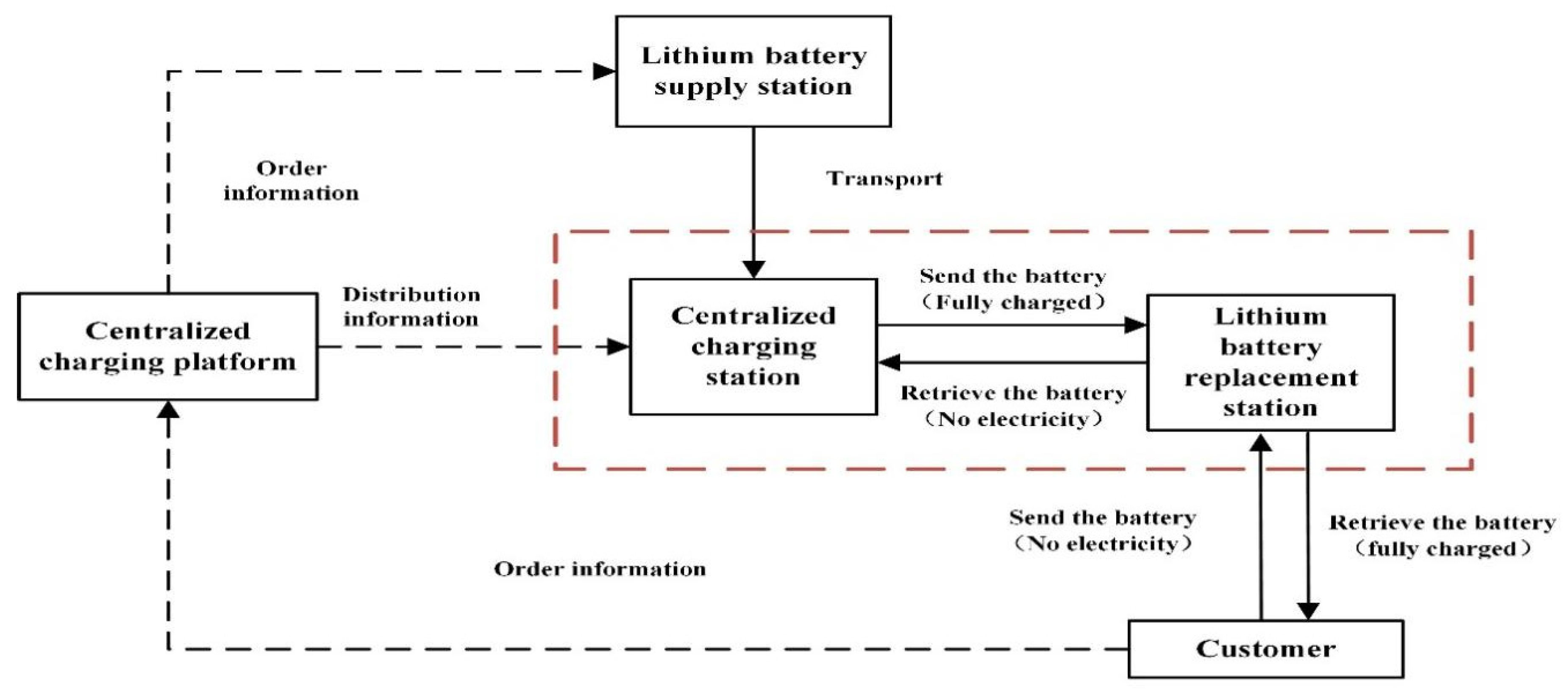
- We first recommend a “centralized charging + unified distribution” power exchange mode, which can help companies take into account safety and cost, optimize their distribution routes, and reduce distribution costs and transportation risks.
- We proposed a dual-objective model to minimize delivery cost and transportation risk, and study a time-windowed vehicle routing problem for simultaneous pickup and delivery of dangerous goods.
- We improved the traditional ant colony algorithm and added the crossover and mutation operations of the genetic algorithm. Based on the R-type data in the Solomon dataset, the effectiveness of the proposed algorithm is verified by comparing the effects of the improved algorithm with the ant colony algorithm, genetic algorithm, and simulated annealing algorithm.
- Change the dual-objective model to a single-objective model by giving different weights to distribution cost and transportation risk. We also explore the optimal distribution paths under different weight combinations to provide decision-making reference for companies with different risk preferences.
2. Literature Review
- (1)
- VRP with Time Windows
- (2)
- VRP with simultaneous pickup and delivery
- (3)
- Vehicle routing problem with simultaneous pickup and delivery with time window constraints (VRPSPDTW)
- (4)
- Research on the path problem of dangerous goods distribution and the solution method
3. Basic Model
3.1. Problem Description and Model Assumptions
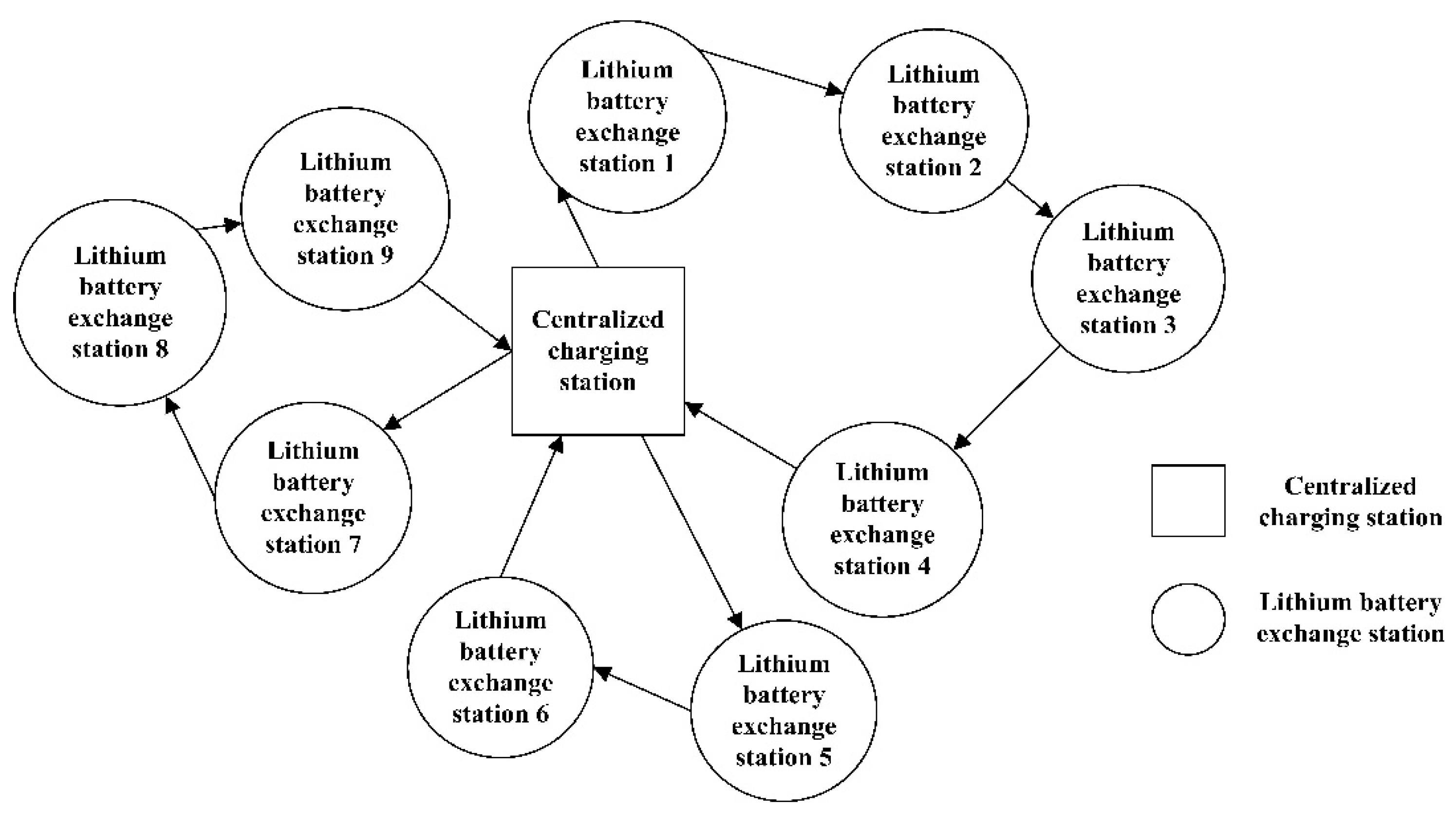
- The “centralized charging + unified distribution” mode of power exchange has been applied on a large scale in a certain area, and the number of batteries can meet the demand of all lithium battery exchange stations.
- There is a centralized charging station (24 h charging service) in the region, the number of vehicles is certain, and the starting and ending points of vehicle distribution are centralized charging stations.
- The location of each lithium battery exchange station and the demand for picking up and delivering lithium batteries are known before the vehicle departs.
- The distance between the centralized charging station and each lithium battery exchange station, the service time, the accident probability of each road section, the accident impact radius, the population density, and the number of people affected are known.
- Each vehicle has the same specification and maximum load capacity. Assume that the number of vehicles is three, and the driving speed is constant at 60 km/h.
- Each lithium battery exchange station is delivered and picked up by only one vehicle and the pickup and delivery demand is met at one time.
- The lithium batteries can be mixed and delivered with the same specifications, and the actual loading capacity of each vehicle cannot exceed the maximum loading capacity of the vehicle.
- Each lithium battery exchange station has a designated service window, and the distribution vehicle needs to provide service within this timeframe.
- The service time of the distribution vehicle at the lithium battery exchange station is not related to the distribution volume.
- The distribution cost only considers variable cost (proportional to the number of miles driven by the vehicle) and time window penalty cost. Fixed costs (constants, including driver’s salary, vehicle insurance, etc.) are not considered for the time being.
3.2. Model Constraint
- (1)
- Distribution cost
- (2)
- Transportation risk
3.3. Multi-Objective Model
4. Ant Colony Genetic Hybrid Algorithm Design and Verification
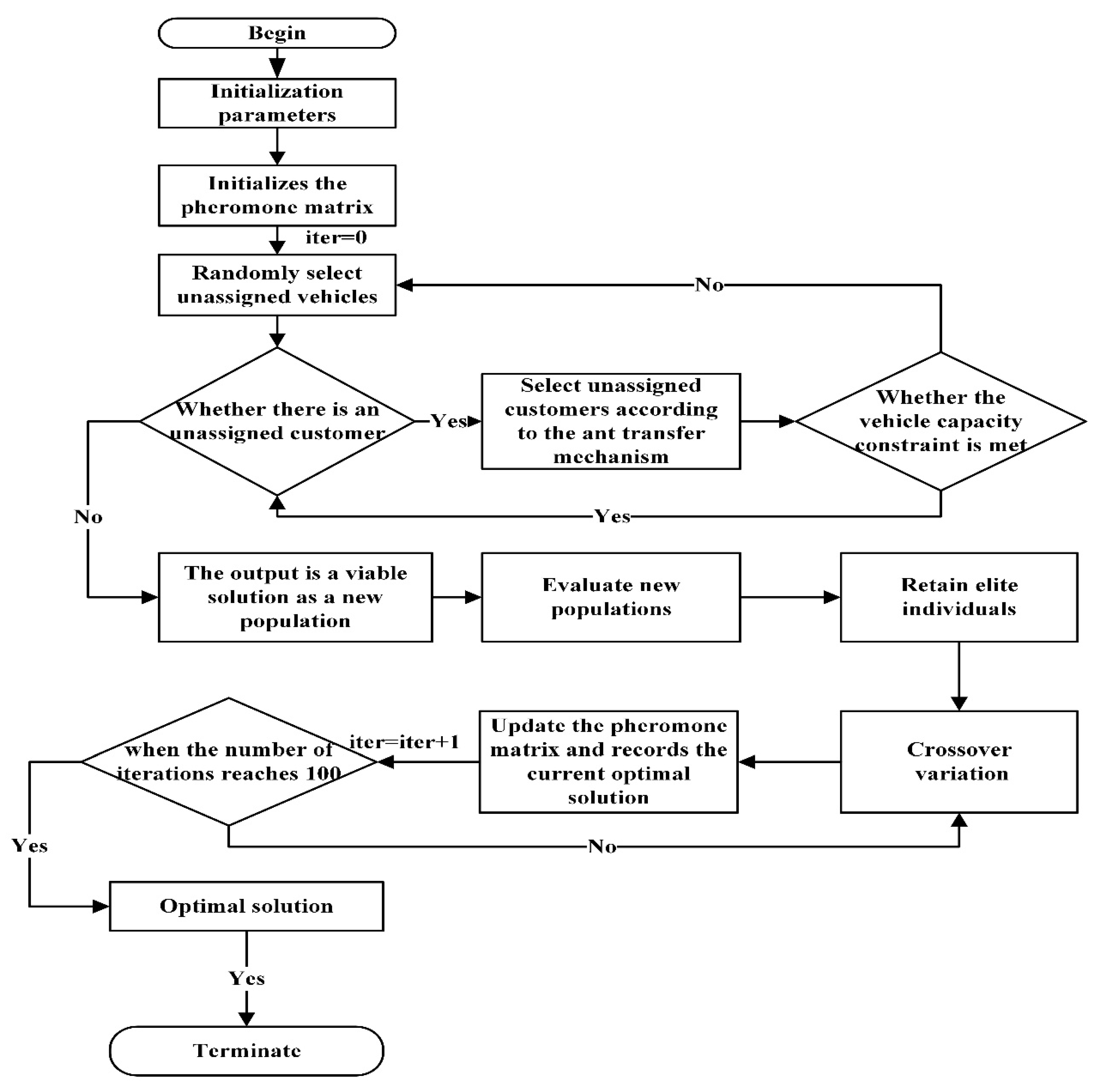
4.1. Algorithm Design
- (1)
- Initialization parameters. Set the initial value of the iteration number iter = 1 and the maximum iteration number iter_max = 100. The definitions and values of other parameters () are shown in Table 4.
- (2)
- Pheromone updating. Set the initial pheromone of all locations to 1, so that the ants have the same probability of crawling to each location. Calculate the length path traversed by the ants, record the current optimal solution, and update the pheromone.
- (3)
- Transfer of ants. When choosing the next place to visit, the ants will use the pheromone concentration on each connection path as a reference. denotes the probability that ant k moves from point i to j at time t.
- (4)
- Load capacity check of the visiting location: if the load constraints are met, continue to visit, otherwise re-select the next place to be visited. The sites visited by the ants are added to the taboo list until the ants have visited all the sites.
- (5)
- Evaluate the new population: In this study, the fitness function was used to evaluate the new population judging the quality of individuals in the group through the objective function. Since the objective function in this study is to minimize the delivery cost and transportation risk, the inverse of the objective function is used as the value of the fitness function.
- (6)
- Crossover and mutation: according to the crossover probability , some genes on the chromosomes corresponding to the two individuals are crossed to generate a new individual. Then, according to the mutation probability , the gene on the chromosome is mutated. Through crossover and mutation, new individuals can be generated to increase population diversity.
4.2. Validity Verification
5. Empirical Analysis
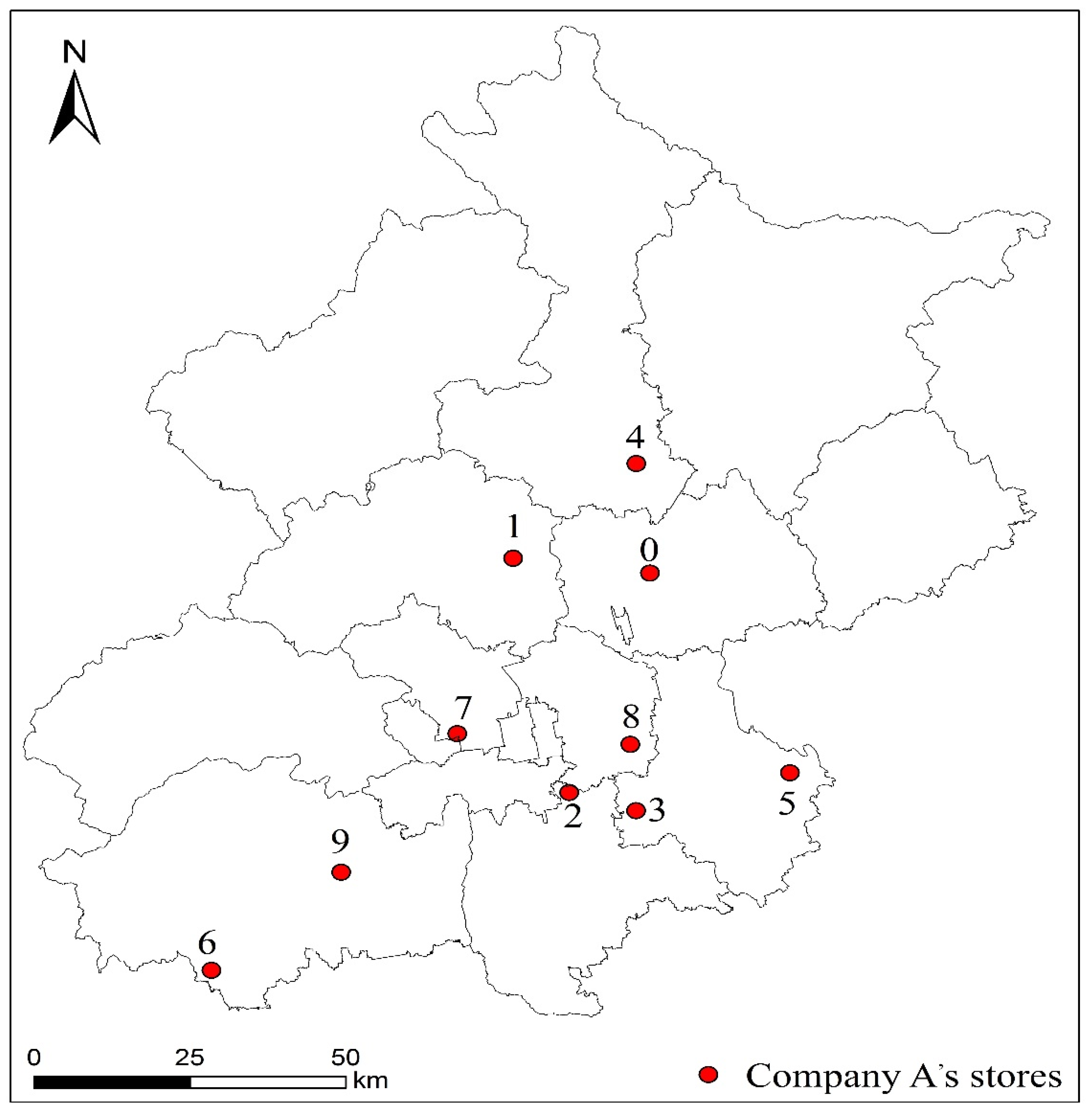
5.1. Case Introduction and Preprocessing
5.2. Parameter Combination Analysis
- (1)
- Information heuristic factor α and the expectation heuristic factor β
- (2)
- Information volatility factor ρ
- (3)
- Crossover operator and variational operator
5.3. Path Preference Analysis
6. Conclusions
Author Contributions
Funding
Institutional Review Board Statement
Informed Consent Statement
Data Availability Statement
Conflicts of Interest
Appendix A

| Sets and Parameters | |
|---|---|
| Centralized charging station | |
| The number of lithium battery exchange stations | |
| The number of delivery vehicles at centralized charging stations | |
| for lithium battery exchange | |
| delivery volume | |
| Delivery vehicle unit distance transportation cost | |
| Unit penalty cost for early arrival | |
| Unit penalty cost for being late | |
| Maximum load capacity of the vehicles. | |
| The radius of influence of the accident | |
| Weighting factor for delivery cost | |
| Weighting factor for transportation risk | |
| 0 | 1 | 2 | 3 | 4 | 5 | 6 | 7 | 8 | 9 | 10 | 11 | 12 | 13 | 14 | 15 | |
|---|---|---|---|---|---|---|---|---|---|---|---|---|---|---|---|---|
| 0 | 0 | 1.13 | 1.76 | 1.44 | 1.51 | 1.45 | 1.84 | 1.22 | 1.64 | 1.06 | 1.48 | 1.90 | 1.43 | 1.27 | 1.01 | 1.39 |
| 1 | 1.13 | 0 | 1.28 | 1.33 | 1.79 | 1.33 | 1.35 | 1.90 | 1.54 | 1.21 | 1.80 | 1.56 | 1.87 | 1.02 | 1.48 | 1.14 |
| 2 | 1.76 | 1.28 | 0 | 1.50 | 1.36 | 1.81 | 1.26 | 1.37 | 1.08 | 1.59 | 1.31 | 1.29 | 1.01 | 1.67 | 1.17 | 1.91 |
| 3 | 1.44 | 1.33 | 1.50 | 0 | 1.56 | 1.28 | 1.75 | 1.09 | 1.37 | 1.61 | 1.35 | 1.93 | 1.26 | 1.43 | 1.61 | 1.69 |
| 4 | 1.51 | 1.79 | 1.36 | 1.56 | 0 | 1.25 | 1.31 | 1.45 | 1.81 | 1.44 | 1.56 | 1.27 | 1.02 | 1.42 | 1.63 | 1.43 |
| 5 | 1.45 | 1.33 | 1.81 | 1.28 | 1.25 | 0 | 1.30 | 1.81 | 1.47 | 1.39 | 1.93 | 1.46 | 1.38 | 1.40 | 1.04 | 1.49 |
| 6 | 1.84 | 1.35 | 1.26 | 1.75 | 1.31 | 1.30 | 0 | 1.21 | 1.08 | 1.32 | 1.69 | 1.64 | 1.50 | 1.83 | 1.05 | 1.73 |
| 7 | 1.22 | 1.90 | 1.37 | 1.09 | 1.45 | 1.81 | 1.21 | 0 | 1.87 | 1.21 | 1.10 | 1.34 | 1.68 | 1.35 | 1.45 | 1.88 |
| 8 | 1.64 | 1.54 | 1.08 | 1.37 | 1.81 | 1.47 | 1.08 | 1.87 | 0 | 1.39 | 1.05 | 1.49 | 1.33 | 1.40 | 1.35 | 1.08 |
| 9 | 1.06 | 1.21 | 1.59 | 1.61 | 1.44 | 1.39 | 1.32 | 1.21 | 1.39 | 0 | 1.33 | 1.47 | 1.45 | 1.05 | 1.46 | 1.39 |
| 10 | 1.48 | 1.80 | 1.31 | 1.35 | 1.56 | 1.93 | 1.69 | 1.10 | 1.05 | 1.33 | 0 | 1.01 | 1.59 | 1.39 | 1.04 | 1.30 |
| 11 | 1.90 | 1.56 | 1.29 | 1.93 | 1.27 | 1.46 | 1.64 | 1.34 | 1.49 | 1.47 | 1.01 | 0 | 1.38 | 1.29 | 1.90 | 1.07 |
| 12 | 1.43 | 1.87 | 1.01 | 1.26 | 1.02 | 1.38 | 1.50 | 1.68 | 1.33 | 1.45 | 1.59 | 1.38 | 0 | 1.28 | 1.42 | 1.47 |
| 13 | 1.27 | 1.02 | 1.67 | 1.43 | 1.42 | 1.40 | 1.83 | 1.35 | 1.40 | 1.05 | 1.39 | 1.29 | 1.28 | 0 | 1.17 | 1.03 |
| 14 | 1.01 | 1.48 | 1.17 | 1.61 | 1.63 | 1.04 | 1.05 | 1.45 | 1.35 | 1.46 | 1.04 | 1.90 | 1.42 | 1.17 | 0 | 1.29 |
| 15 | 1.39 | 1.14 | 1.91 | 1.69 | 1.43 | 1.49 | 1.73 | 1.88 | 1.08 | 1.39 | 1.30 | 1.07 | 1.47 | 1.03 | 1.29 | 0 |
| 0 | 1 | 2 | 3 | 4 | 5 | 6 | 7 | 8 | 9 | 10 | 11 | 12 | 13 | 14 | 15 | |
|---|---|---|---|---|---|---|---|---|---|---|---|---|---|---|---|---|
| 0 | 0 | 572 | 338 | 574 | 490 | 329 | 383 | 464 | 588 | 590 | 347 | 592 | 588 | 446 | 540 | 342 |
| 1 | 572 | 0 | 538 | 588 | 497 | 310 | 555 | 581 | 504 | 528 | 523 | 418 | 497 | 351 | 512 | 309 |
| 2 | 338 | 538 | 0 | 547 | 509 | 395 | 586 | 310 | 432 | 414 | 530 | 539 | 356 | 447 | 434 | 494 |
| 3 | 574 | 588 | 547 | 0 | 497 | 348 | 335 | 450 | 588 | 402 | 476 | 367 | 526 | 376 | 452 | 510 |
| 4 | 490 | 497 | 509 | 497 | 0 | 377 | 553 | 376 | 545 | 373 | 579 | 405 | 359 | 375 | 485 | 442 |
| 5 | 329 | 310 | 395 | 348 | 377 | 0 | 527 | 526 | 414 | 470 | 322 | 316 | 459 | 534 | 581 | 339 |
| 6 | 383 | 555 | 586 | 335 | 553 | 527 | 0 | 459 | 349 | 481 | 379 | 496 | 507 | 525 | 435 | 325 |
| 7 | 464 | 581 | 310 | 450 | 376 | 526 | 459 | 0 | 332 | 589 | 300 | 533 | 546 | 561 | 325 | 420 |
| 8 | 588 | 504 | 432 | 588 | 545 | 414 | 349 | 332 | 0 | 474 | 465 | 343 | 556 | 487 | 405 | 454 |
| 9 | 590 | 528 | 414 | 402 | 373 | 470 | 481 | 589 | 474 | 0 | 447 | 589 | 556 | 487 | 405 | 454 |
| 10 | 347 | 523 | 530 | 476 | 579 | 322 | 379 | 300 | 465 | 447 | 0 | 406 | 547 | 304 | 312 | 350 |
| 11 | 592 | 418 | 539 | 367 | 405 | 316 | 496 | 533 | 343 | 589 | 406 | 0 | 534 | 324 | 579 | 533 |
| 12 | 588 | 497 | 356 | 526 | 359 | 459 | 507 | 546 | 556 | 556 | 547 | 534 | 0 | 582 | 563 | 465 |
| 13 | 446 | 351 | 447 | 376 | 375 | 534 | 525 | 561 | 487 | 487 | 304 | 324 | 582 | 0 | 429 | 355 |
| 14 | 540 | 512 | 434 | 452 | 485 | 581 | 435 | 325 | 405 | 405 | 312 | 579 | 563 | 429 | 0 | 452 |
| 15 | 342 | 309 | 494 | 510 | 442 | 339 | 325 | 420 | 454 | 454 | 350 | 533 | 465 | 355 | 452 | 0 |
| Number | Store Name | Longitude | Latitude |
|---|---|---|---|
| 0 | Company A warehouse | 116.650873 | 40.154191 |
| 1 | Store 1 | 116.394265 | 40.200878 |
| 2 | Store 2 | 116.441387 | 39.810124 |
| 3 | Store 3 | 116.563345 | 39.769598 |
| 4 | Store 4 | 116.653201 | 40.334977 |
| 5 | Store 5 | 116.864538 | 39.805573 |
| 6 | Store 6 | 115.721256 | 39.577671 |
| 7 | Store 7 | 116.244193 | 39.923892 |
| 8 | Store 8 | 116.569297 | 39.878586 |
| 9 | Store 9 | 115.990276 | 39.71676 |
References
- China Bicycle Association. Available online: http://www.china-bicycle.com/ (accessed on 3 February 2022).
- Huajing Intelligence Network. Available online: https://www.huaon.com/channel/trend/797511.html (accessed on 14 April 2022).
- GB 17761-2018; E-Bike Safety Technical Specifications. Standards Press of China: Beijing, China, 2018.
- Shuai, C.Y.; Yang, F.; OuYang, X.; Xu, G. Data-driven demand forecasting for electric bicycle power exchange. Transp. Syst. Eng. Inf. 2021, 21, 173–179. [Google Scholar]
- Ministry of Transport of the People’s Republic of China. Report on Sustainable Transport in China. Available online: https://www.mot.gov.cn/zhuanti/transport/chengguowj/202110/P020211027595442474938.pdf (accessed on 3 February 2022).
- Fire and Rescue Department Ministry Emergency Management. Available online: https://www.119.gov.cn/article/46TiYamnnrs (accessed on 3 February 2022).
- Dai, J.C. Comparison of electric vehicle whole vehicle charging mode and centralized charging + power exchange mode. Power Demand Side Manag. 2014, 16, 57–60. [Google Scholar]
- Dantzig, G.B.; Ramser, J.H. The truck dispatching problem. Manag. Sci. 1959, 6, 80–91. [Google Scholar] [CrossRef]
- Pérez-Rodríguez, R.; Hernández-Aguirre, A. A hybrid estimation of distribution algorithm for the vehicle routing problem with time windows. Comput. Ind. Eng. 2019, 130, 75–96. [Google Scholar] [CrossRef]
- Konstantakopoulos, G.D.; Gayialis, S.P.; Kechagias, E.P. Vehicle routing problem and related algorithms for logistics distribution: A literature review and classification. Oper. Res. 2022, 22, 2033–2062. [Google Scholar] [CrossRef]
- Solomon, M.M. Algorithms for the vehicle routing and scheduling problems with time window constraints. Oper. Res. 1987, 35, 254–265. [Google Scholar] [CrossRef] [Green Version]
- Koskosidis, Y.A.; Powell, W.B.; Solomon, M.M. An optimization-based heuristic for vehicle routing and scheduling with soft time window constraints. Transp. Sci. 1992, 26, 69–85. [Google Scholar] [CrossRef]
- Chiang, W.C.; Russell, R.A. A metaheuristic for the vehicle-routing problem with soft time windows. J. Oper. Res. Societ. 2004, 55, 1298–1310. [Google Scholar] [CrossRef]
- Bae, H.; Moon, I. Multi-depot vehicle routing problem with time windows considering delivery and installation vehicles. Appl. Math. Model. 2016, 40, 6536–6549. [Google Scholar] [CrossRef]
- Ye, Y.; Zhang, H.Z. Wolfpack algorithm for solving vehicle path problems with time windows. Highw. Traffic Technol. 2017, 34, 100–107. [Google Scholar]
- Sun, J.C.; Li, D. Open vehicle path problem based on improved firefly algorithm. Pract. Underst. Math. 2018, 48, 182–190. [Google Scholar]
- Wu, L.B.; He, Z.J.; Chen, Y.J.; Wu, D.; Cui, J.Q. Brainstorming-Based Ant Colony Optimization for Vehicle Routing With Soft Time Windows. IEEE Access 2019, 7, 19643–19652. [Google Scholar]
- He, M.L.; Wei, Z.X.; Wu, X.H.; Peng, Y.T. An improved ant colony based algorithm for solving vehicle path problems with soft time windows. Comput. Integr. Manuf. Syst. 2021, 1–14. Available online: https://kns.cnki.net/kcms/detail/detail.aspx?dbcode=CAPJ&dbname=CAPJLAST&filename=JSJJ20210723002&uniplatform=NZKPT&v=EfDktvpY4SAJDRUlkmtxMlt5c853-MY6QWqILRG8ZdYmDW_TBi_7fAm7iPg60Br8 (accessed on 3 February 2022).
- Yu, Y.; Wang, S.; Wang, J.; Huang, M. A branch-and-price algorithm for the heterogeneous fleet green vehicle routing problem with time windows. Transp. Res. Part B Methodol. 2019, 122, 511–527. [Google Scholar] [CrossRef]
- Wang, J.; Weng, T.; Zhang, Q. A two-stage multiobjective evolutionary algorithm for multiobjective multidepot vehicle routing problem with time windows. IEEE Trans. Cybern. 2018, 49, 2467–2478. [Google Scholar] [CrossRef] [PubMed]
- Song, M.; Li, J.; Han, Y.; Han, Y.-Y.; Liu, L.; Sun, Q. Metaheuristics for solving the vehicle routing problem with the time windows and energy consumption in cold chain logistics. Appl. Soft Comput. 2020, 95, 106561. [Google Scholar] [CrossRef]
- Goetschalckx, M.; Jacobs-blecha, C. The vehicle routing problem with back hauls. Eur. J. Oper. Res. 1987, 42, 39–51. [Google Scholar] [CrossRef]
- Min, H. The multiple vehicle routing problem with simultaneous delivery and pick up points. Transp. Res. Part. A Gen. 1989, 23, 377–386. [Google Scholar] [CrossRef]
- Reil, S.; Bortfeldt, A.; Mönch, L. Heuristics for vehicle routing problems with backhauls, time windows, and 3D loading constraints. Eur. J. Oper. Res. 2018, 266, 877–894. [Google Scholar] [CrossRef]
- Koç, Ç.; Laporte, G.; Tükenmez, İ. A review of vehicle routing with simultaneous pickup and delivery. Comput. Oper. Res. 2020, 122, 104987. [Google Scholar] [CrossRef]
- Kalayci, C.B.; Kaya, C. An ant colony system empowered variable neighborhood search algorithm for the vehicle routing problem with simultaneous pickup and delivery. Expert Syst. Appl. 2016, 66, 163–175. [Google Scholar] [CrossRef]
- Islam, M.A.; Gajpal, Y.; ElMekkawy, T.Y. Hybrid particle swarm optimization algorithm for solving the clustered vehicle routing problem. Appl. Soft Comput. 2021, 110, 107655. [Google Scholar] [CrossRef]
- Goksal, F.P.; Karaoglan, I.; Altiparmak, F. A hybrid discrete particle swarm optimization for vehicle routing problem with simultaneous pickup and delivery. Comput. Ind. Eng. 2013, 65, 39–53. [Google Scholar] [CrossRef]
- Avci, M.; Topaloglu, S. An adaptive local search algorithm for vehicle routing problem with simultaneous and mixed pickups and deliveries. Comput. Ind. Eng. 2015, 83, 15–29. [Google Scholar] [CrossRef]
- Avci, M.; Topaloglu, S. A hybrid metaheuristic algorithm for heterogeneous vehicle routing problem with simultaneous pickup and delivery. Expert Syst. Appl. 2016, 53, 160–171. [Google Scholar] [CrossRef]
- Ni, L.; Liu, K.P.; Tu, Z.G. Urban courier co-delivery path optimization considering simultaneous pickup and delivery. J. Chongqing Univ. 2017, 40, 30–39. [Google Scholar]
- Chen, X.Q.; Hu, D.W.; Yang, Q.Q.; Hu, H.; Gao, Y. Improved ant colony algorithm for multi-objective simultaneous delivery vehicle path problem. Control Theory Appl. 2018, 35, 1347–1356. [Google Scholar]
- Ma, Y.F.; Yan, F.; Kang, K.; Li, Z.M. Uncertain simultaneous pickup delivery vehicle path problem and particle swarm algorithm research. Oper. Res. Manag. 2018, 27, 73–83. [Google Scholar]
- Ren, T.; Luo, T.Y.; Gu, Z.H.; Hu, Z.Q.; Jia, B.B.; Xing, L.N. Urban logistics common distribution path optimization considering simultaneous pickup and delivery. Comput. Integr. Manuf. Syst. 2022, 1–18. Available online: https://kns.cnki.net/kcms/detail/detail.aspx?dbcode=CAPJ&dbname=CAPJLAST&filename=JSJJ20220315000&uniplatform=NZKPT&v=RxFrS6Ig2zID5j-2re_ca_HUwv4q5cjDEfQHzf8ervf8NyXtmHojlHxPnWaoENOr (accessed on 3 February 2022).
- Wang, L.Y.; Song, Y.B. Multiple Charging Station Location-Routing Problem with Time Window of Electric Vehicle. J. Eng. Sci. Technol. Rev. 2015, 8, 190–201. [Google Scholar]
- Wang, C.; Mu, D.; Zhao, F.; Sutherland, J.W. A parallel simulated annealing method for the vehicle routing problem with simultaneous pickup–delivery and time windows. Comput. Ind. Eng. 2015, 83, 111–122. [Google Scholar] [CrossRef]
- Zhang, Q.H.; Wu, S.P. Modeling of simultaneous delivery vehicle path problem with time window and modal solution algorithm. Comput. Appl. 2020, 40, 1097–1103. [Google Scholar]
- Zhang, X.F.; Hu, R.; Qian, B. Superheuristic distribution estimation algorithm for solving simultaneous delivery vehicle path problems with soft time windows. Control. Theory Appl. 2021, 38, 1427–1441. [Google Scholar]
- Hornstra, R.P.; Silva, A.; Roodbergen, K.J.; Coelho, L.C. The vehicle routing problem with simultaneous pickup and delivery and handling costs. Comput. Oper. Res. 2020, 115, 104858. [Google Scholar] [CrossRef]
- Yan, J.; Chang, L.; Wang, L.L.; Zhao, T. Algorithm for solving the simultaneous pickup and delivery vehicle path problem with time windows. Ind. Eng. 2021, 24, 72–76. [Google Scholar]
- Ahkamiraad, A.; Wang, Y. Capacitated and multiple cross-docked vehicle routing problem with pickup, delivery, and time windows. Comput. Ind. Eng. 2018, 119, 76–84. [Google Scholar] [CrossRef]
- Lagos, C.; Guerrero, G.; Cabrera, E.; Moltedo, A.; Johnson, F.; Paredes, F. An improved particle swarm optimization algorithm for the VRP with simultaneous pickup and delivery and time windows. IEEE Lat. Am. Trans. 2018, 16, 1732–1740. [Google Scholar] [CrossRef]
- Zhang, S.Z.; Chen, T.T.; Sun, R.T.; Bai, X.; Gao, C. Path optimization of dangerous goods transportation vehicles considering cargo capacity. J. Wuhan Univ. Technol. (Inf. Manag. Eng. Ed.) 2020, 42, 290–297. [Google Scholar]
- Erkut, E.; Ingolfsson, A. Transport risk models for hazardous materials: Revisited. Oper. Res. Lett. 2005, 3, 81–89. [Google Scholar] [CrossRef]
- Xin, C.L.; Meng, J.; Zhang, J.W.; Feng, Q.R. A review of hazardous materials transportation route optimization problems. Chin. J. Saf. Sci. 2018, 28, 102–107. [Google Scholar]
- Kara, B.Y.; Verter, V. Designing a road network for hazardous materials transportation. Transp. Sci. 2004, 38, 188–196. [Google Scholar] [CrossRef] [Green Version]
- Zografos, K.G.; Androutsopoulos, K.N. A heuristic algorithm for solving hazardous materials distribution problems. Eur. J. Oper. Res. 2004, 152, 507–519. [Google Scholar] [CrossRef]
- Androutsopoulos, K.N.; Zografos, K.G. Solving the bicriterion routing and scheduling problem for hazardous materials distribution. Transp. Res. Part. C Emerg. Technol. 2010, 18, 713–726. [Google Scholar] [CrossRef] [Green Version]
- Chai, X.; He, R.C.; Ma, C.C. Multi-objective optimization of hazardous materials transportation vehicle path problem. Chin. J. Saf. Sci. 2015, 25, 84–90. [Google Scholar]
- Zhang, M.; Wang, N.M. Research on path optimization of dangerous goods transportation vehicles for major accident avoidance. Oper. Res. Manag. 2018, 27, 1–9. [Google Scholar]
- Li, L.; Deng, Y.T.; Mou, L.L. Research on optimization of dangerous goods transportation path based on improved NSGA-II algorithm. Saf. Environ. Eng. 2021, 28, 111–117. [Google Scholar]
- Erkut, E.; Verter, V. Modeling of transport risk for hazardous materials. Oper. Res. 1998, 46, 625–642. [Google Scholar] [CrossRef] [Green Version]
- Teng, Y.; Sun, L.J.; Zhou, Y.X. A multi-model vehicle path optimization method considering the risk of hazardous materials transportation. Syst. Eng. 2020, 38, 93–102. [Google Scholar]
- Kazantzi, V.; Kazantzis, N.; Gerogiannis, V.C. Risk informed optimization of a hazardous material multi-periodic transportation model. J. Loss Prev. Process. Ind. 2011, 24, 767–773. [Google Scholar] [CrossRef]
- Zhou, R.; Shen, W.L.; Liu, M.Z.; Zhao, H. Hybrid discrete particle swarm optimization algorithm for integrated vehicle path problems with time windows for loading and unloading. China Mech. Eng. 2016, 27, 494–502. [Google Scholar]
- Ye, Z.W.; Zheng, Z.B. Configuration of Parameters α, β and ρ in Ant Algorithm. Geomat. Inf. Sci. Wuhan Univ. 2004, 29, 597–601. [Google Scholar]
- Li, Z.X.; Li, J.X. Quickly Calculate the Distance between Two Points and Measurement Error Based on Latitude and Longitude. Geomat. Spat. Inf. Technol. 2013, 36, 235–237. [Google Scholar]

| Literature | Problem | Algorithm | Objective |
|---|---|---|---|
| Bae et al. [14] | Multi-depot vehicle routing problem with time windows (MDVRPTW) | Heuristic algorithm and a hybrid genetic algorithm | Minimize the total relevant costs |
| Ye et al. [15] | VRPTW | Wolf pack algorithm | Minimum total transportation cost |
| Sun et al. [16] | Multi-depot open vehicle routing problem with soft time windows (MDOVRPTW) | Improved glowworm swarm optimization (GSO) | Minimum total cost |
| Wu et al. [17] | VRPSTW | Optimized ACO | Minimum total transportation cost |
| He et al. [18] | VRPSTW | Optimized ACO | Minimize delivery costs |
| Yu et al. [19] | Heterogeneous fleet green vehicle routing problem with time windows (HFGVRPTW) | Multi-vehicle approximate dynamic programming (MVADP) | The branches and computational time |
| Wang et al. [20] | Multi-depot VRPTW (MDVRPTW) | Two-stage multi-objective evolutionary algorithm | Minimize the number of vehicles, total travel distance, makespan, total waiting time, and total delay time |
| Song et al. [21] | VRPTW in cold chain logistics | Improved artificial fish swarm (IAFS) | Minimize the fixed cost and the energy consumptions |
| Literature | Application Scenarios | Algorithm | Objective |
|---|---|---|---|
| Goksal et al. [28] | VRPSPD | Optimized PSO | Extend the algorithm for solving VRPSPD |
| Avci et al. [29,30] | VRPSD with multiple vehicle models | Hybrid Local Search Algorithm | Extend the algorithm for solving VRPSPD |
| Ni et al. [31] | Multiple courier companies jointly deliver | Optimized ACO | Minimize total delivery costs |
| Chen et al. [32] | Dual-objective VRPSPD model considering both vehicle capacity and distance constraints | Optimized ACO | Minimize the maximum length difference routes and minimize transportation cost |
| Ma et al. [33] | Uncertain simultaneous pickup and delivery vehicle routing problem | Optimized PSO | Lowest operating costs and highest customer satisfaction |
| Ren et al. [34] | The problem of picking up and delivering orders in the same city | Optimized GA | Minimize total cost |
| Literature | Algorithm | Objective |
|---|---|---|
| Wang et al. [36] | Simulated annealing (SA) algorithm | Minimize the routing cost |
| Zhang, Q.H et al. [37] | Memetic algorithm | Minimum the number of vehicles and shortest vehicle travel path |
| Zhang, S.Z et al. [38] | Optimized TSA | Minimize the total cost including time penalty cost |
| Hornstra et al. [39] | Adaptive large neighborhood search (ALNS) | Minimize the total processing cost |
| Yan et al. [40] | K-means-ACO | Minimize the total travel cost during return and delivery service |
| Ahkamiraad et al. [41] | A hybrid of the genetic algorithm and particle swarm optimization (HGP) | Minimize the transportation and fixed costs |
| Lagos et al. [42] | PSO | Minimize the total distance of the paths and serving customers’ demands |
| Parameters | Parameter Meaning | Parameter Value |
|---|---|---|
| Population size | 10 | |
| Information heuristic factor | 1 | |
| Expectation heuristic factor | 5 | |
| Information volatility factor | 0.75 | |
| Total pheromone release | 10 | |
| Crossover probability | 0.5 | |
| Mutation probability | 0.1 | |
| Delivery vehicle unit distance transportation cost | 3 CNY/km | |
| Unit penalty cost for early arrival | 20 CNY/h | |
| Unit penalty cost for being late | CNY/h | |
| The radius of influence of the accident | 0.1 km |
| Serial Number | Customer Coordinates | Delivery Quantity (Pieces) | Pickup Quantity (Pieces) | Time Window (min) | Service Time (min) |
|---|---|---|---|---|---|
| 0 | (35, 35) | ||||
| 1 | (41, 49) | 8 | 2 | [161, 171] | 10 |
| 2 | (35, 17) | 3 | 4 | [50, 60] | 10 |
| 3 | (55, 45) | 11 | 2 | [116, 126] | 10 |
| 4 | (55, 20) | 7 | 12 | [149, 159] | 10 |
| 5 | (15, 30) | 13 | 13 | [34, 44] | 10 |
| 6 | (25, 30) | 3 | 0 | [99, 109] | 10 |
| 7 | (20, 50) | 2 | 3 | [81, 91] | 10 |
| 8 | (10, 43) | 2 | 7 | [95, 105] | 10 |
| 9 | (55, 60) | 15 | 1 | [97, 107] | 10 |
| 10 | (30, 60) | 8 | 8 | [124, 134] | 10 |
| 11 | (20, 65) | 4 | 8 | [67, 77] | 10 |
| 12 | (50, 35) | 13 | 6 | [63, 73] | 10 |
| 13 | (30, 25) | 19 | 4 | [159, 169] | 10 |
| 14 | (15, 10) | 13 | 7 | [32, 42] | 10 |
| 15 | (30, 5) | 1 | 7 | [61, 71] | 10 |
| Algorithm | Number of Iterations | |||||
|---|---|---|---|---|---|---|
| 0.8–0.2 | 0.6–0.4 | 0.5–0.5 | 0.4–0.6 | 0.2–0.8 | ||
| ACO-GA | 1008.23 | 889.22 | 789.14 | 708.29 | 556.42 | 35 |
| ACO | 1015.13 | 865.88 | 801.90 | 725.51 | 560.19 | 45 |
| GA | 1471.99 | 1232.84 | 1200.59 | 1007.75 | 767.58 | 68 |
| SAA | 1547.08 | 1377.72 | 1202.06 | 983.86 | 728.12 | 89 |
| Stores No. | 0 | 1 | 2 | 3 | 4 | 5 | 6 | 7 | 8 | 9 |
|---|---|---|---|---|---|---|---|---|---|---|
| 0 | 0 | 22.4 | 42.2 | 43.4 | 20.1 | 42.8 | 102.3 | 43.0 | 31.4 | 72.3 |
| 1 | 0 | 43.6 | 50.1 | 26.5 | 59.4 | 89.2 | 33.3 | 38.8 | 63.8 | |
| 2 | 0 | 11.4 | 61.1 | 36.1 | 66.7 | 21.1 | 13.3 | 39.9 | ||
| 3 | 0 | 63.3 | 26.1 | 75.3 | 32.2 | 12.1 | 49.3 | |||
| 4 | 0 | 61.5 | 11.5 | 57.4 | 51.2 | 88.8 | ||||
| 5 | 0 | 100.9 | 54.6 | 26.5 | 75.3 | |||||
| 6 | 0 | 59.1 | 80.0 | 27.8 | ||||||
| 7 | 0 | 28.2 | 31.6 | |||||||
| 8 | 0 | 52.6 | ||||||||
| 9 | 0 |
| Serial | Store Name | Delivery | Pickup | Time | Service Time |
|---|---|---|---|---|---|
| Number | Quantity (Pieces) | Quantity (Pieces) | Window (min) | (min) | |
| 0 | Company A warehouse | ||||
| 1 | Store 1 | 10 | 2 | [7:30–7:45] | 8 |
| 2 | Store 2 | 7 | 10 | [7:45–8:00] | 10 |
| 3 | Store 3 | 6 | 3 | [8:10–8:35] | 5 |
| 4 | Store 4 | 5 | 6 | [7:05–7:20] | 5 |
| 5 | Store 5 | 4 | 14 | [8:15–8:25] | 10 |
| 6 | Store 6 | 14 | 7 | [8:30–9:00] | 10 |
| 7 | Store 7 | 11 | 6 | [7:55–8:10] | 9 |
| 8 | Store 8 | 6 | 3 | [7:50–8:15] | 6 |
| 9 | Store 9 | 14 | 2 | [8:00–8:30] | 7 |
| α | β | Average Cost (CNY) | Average Risk | Weighted Objective Function Value (CNY) | Number of Iterations to Reach Convergence | Time (s) |
|---|---|---|---|---|---|---|
| 0 | 5 | 32.30 | 5.78 | 19.04 | 89 | 11.70 |
| 0.5 | 5 | 37.84 | 5.76 | 21.80 | 32 | 12.91 |
| 1 | 5 | 34.91 | 5.99 | 20.45 | 79 | 12.57 |
| 2 | 5 | 21.37 | 5.41 | 13.88 | 7 | 11.73 |
| α | β | Average Cost (CNY) | Average Risk | Weighted Objective Function Value | Number of Iterations to Reach Convergence | Time (s) |
|---|---|---|---|---|---|---|
| 2 | 0 | 41.65 | 8.68 | 24.90 | 20 | 13.83 |
| 2 | 2 | 33.08 | 6.25 | 19.66 | 38 | 17.60 |
| 2 | 4 | 34.33 | 5.66 | 20.00 | 6 | 16.20 |
| 2 | 5 | 32.89 | 5.87 | 19.38 | 5 | 11.86 |
| ρ | Average Cost (CNY) | Average Risk | Weighted Objective Function Value | Number of Iterations to Reach Convergence | Time (s) |
|---|---|---|---|---|---|
| 0.2 | 36.11 | 5.69 | 20.90 | 52 | 13.78 |
| 0.4 | 33.88 | 5.67 | 19.78 | 42 | 12.03 |
| 0.6 | 38.17 | 5.94 | 22.06 | 57 | 12.10 |
| 0.8 | 32.36 | 5.90 | 19.13 | 36 | 13.29 |
| Average Cost (CNY) | Average Risk | Weighted Objective Function Value | Number of Iterations to Reach Convergence | Time (s) | ||
|---|---|---|---|---|---|---|
| 0.2 | 1 | 28.11 | 5.85 | 16.98 | 23 | 16.11 |
| 0.4 | 1 | 29.53 | 5.98 | 17.75 | 56 | 13.06 |
| 0.6 | 1 | 28.29 | 5.77 | 17.03 | 71 | 14.64 |
| 0.8 | 1 | 29.64 | 5.92 | 17.78 | 95 | 12.35 |
| Average Cost (CNY) | Average Risk | Weighted Objective Function Value | Number of Iterations to Reach Convergence | Time (s) | ||
|---|---|---|---|---|---|---|
| 1 | 0.2 | 33.75 | 5.89 | 19.82 | 88 | 13.23 |
| 1 | 0.4 | 30.69 | 5.46 | 18.08 | 31 | 13.76 |
| 1 | 0.6 | 28.85 | 5.79 | 17.32 | 14 | 14.32 |
| 1 | 0.8 | 28.98 | 5.85 | 17.42 | 17 | 12.75 |
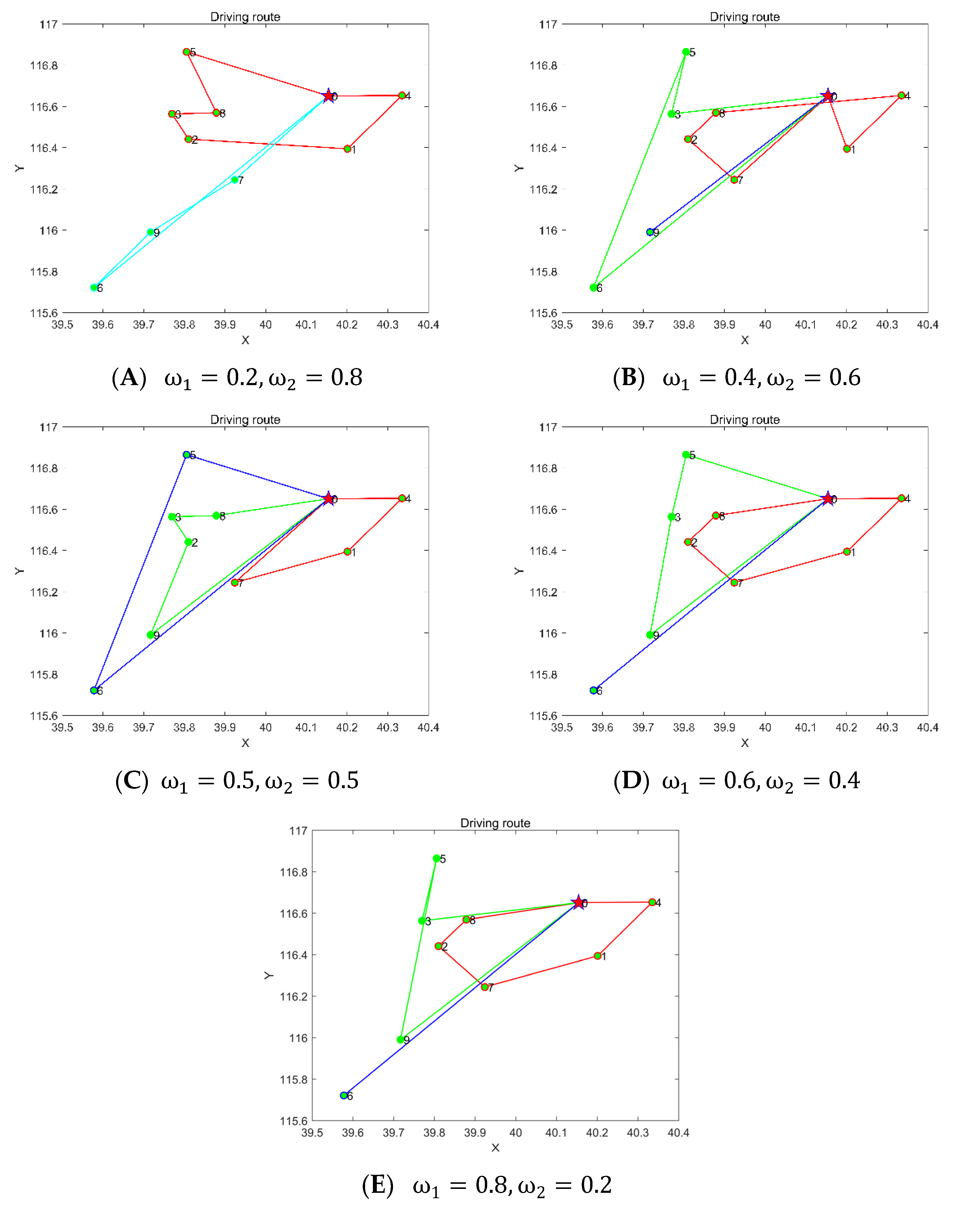
| Strategy | Weights | Optimal Path | |||||||
|---|---|---|---|---|---|---|---|---|---|
| Vehicle 1 | Vehicle 2 | Vehicle 3 | Normalized Objective Function Value | Distribution Cost | Shipping Risks | Programs Preference | |||
| A | 0.2 | 0.8 | 0→4→1 →2→3→8→5→0 | 0→7→9 →6→0 | 0.76 | 60.14 | 5.40 | Very concerned about risk | |
| B | 0.4 | 0.6 | 0→1→4 →8→2→7→0 | 0→3→5 →6→0 | 0→5→3 →2→0 | 0.47 | 29.34 | 8.67 | More concerned about risk |
| C | 0.5 | 0.5 | 0→4→1 →7→0 | 0→8→3 →2→9→0 | 0→5→6 →0 | 0.83 | 55.17 | 8.08 | Intentional risk and cost |
| D | 0.6 | 0.4 | 0→4→1 →7→2→8→0 | 0→5→3 →9→0 | 0→6→0 | 0.42 | 29.88 | 7.85 | More concerned about cost |
| E | 0.8 | 0.2 | 0→4→1 →7→2→8→0 | 0→3→5 →9→0 | 0→6→0 | 0.80 | 28.40 | 8.51 | Very concerned about cost |
Publisher’s Note: MDPI stays neutral with regard to jurisdictional claims in published maps and institutional affiliations. |
© 2022 by the authors. Licensee MDPI, Basel, Switzerland. This article is an open access article distributed under the terms and conditions of the Creative Commons Attribution (CC BY) license (https://creativecommons.org/licenses/by/4.0/).
Share and Cite
Chen, L.; Ma, H.; Wang, Y.; Li, F. Vehicle Routing Problem for the Simultaneous Pickup and Delivery of Lithium Batteries of Small Power Vehicles under Charging and Swapping Mode. Sustainability 2022, 14, 9883. https://doi.org/10.3390/su14169883
Chen L, Ma H, Wang Y, Li F. Vehicle Routing Problem for the Simultaneous Pickup and Delivery of Lithium Batteries of Small Power Vehicles under Charging and Swapping Mode. Sustainability. 2022; 14(16):9883. https://doi.org/10.3390/su14169883
Chicago/Turabian StyleChen, Lei, Haiyan Ma, Yi Wang, and Feng Li. 2022. "Vehicle Routing Problem for the Simultaneous Pickup and Delivery of Lithium Batteries of Small Power Vehicles under Charging and Swapping Mode" Sustainability 14, no. 16: 9883. https://doi.org/10.3390/su14169883
APA StyleChen, L., Ma, H., Wang, Y., & Li, F. (2022). Vehicle Routing Problem for the Simultaneous Pickup and Delivery of Lithium Batteries of Small Power Vehicles under Charging and Swapping Mode. Sustainability, 14(16), 9883. https://doi.org/10.3390/su14169883