
Identifying Population Hollowing Out Regions and Their Dynamic Characteristics across Central China

 ,
, 
Abstract
:1. Introduction
2. Study Area and Materials
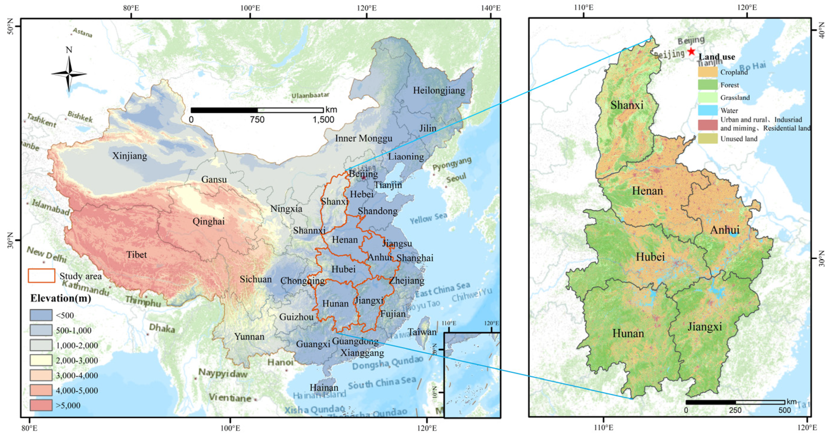
2.1. Study Area
2.2. Data Sources and Pretreatment
3. Methods
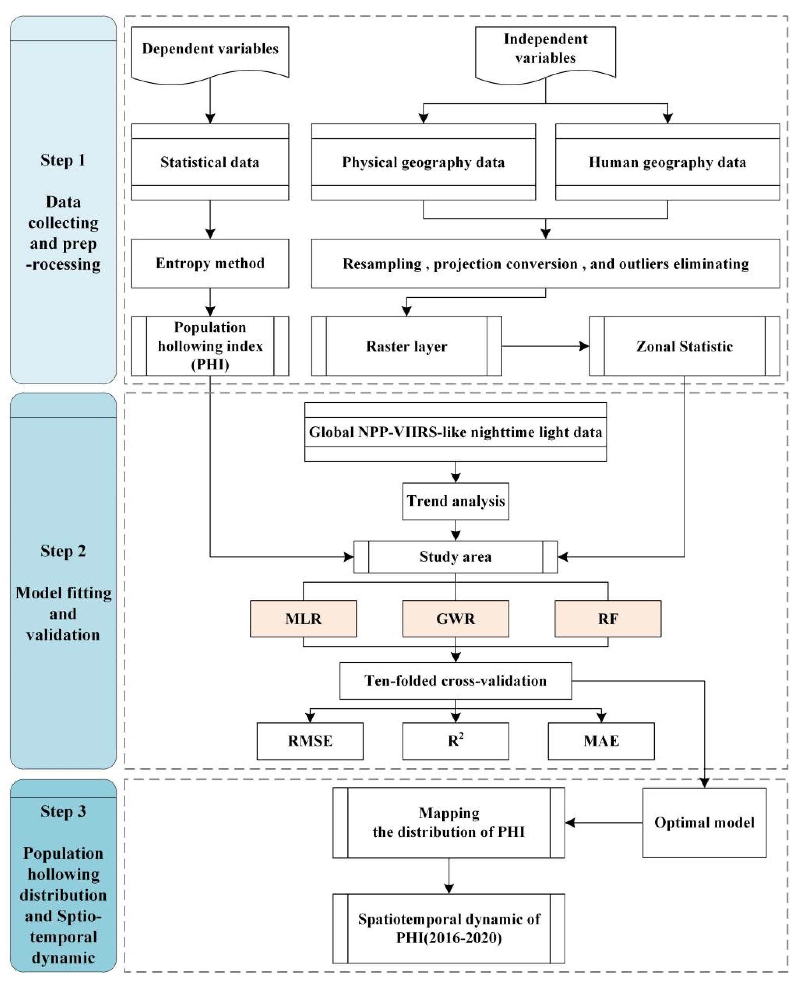
3.1. Workflow
3.2. Calculation of Population Hollowing Index Based on Statistical Data
3.3. Fitting PHI Prediction Models on a Political Boundary Scale
3.3.1. Geographically Weighted Regression (GWR)
3.3.2. Regression Model
3.3.3. Random Forest (RF)
3.3.4. Validation
3.4. Detecting the Distribution and the Dynamic of Population Hollowing
3.4.1. Mapping the PHI on a Grid-Scale
3.4.2. Detecting the Dynamic of PHI
4. Results
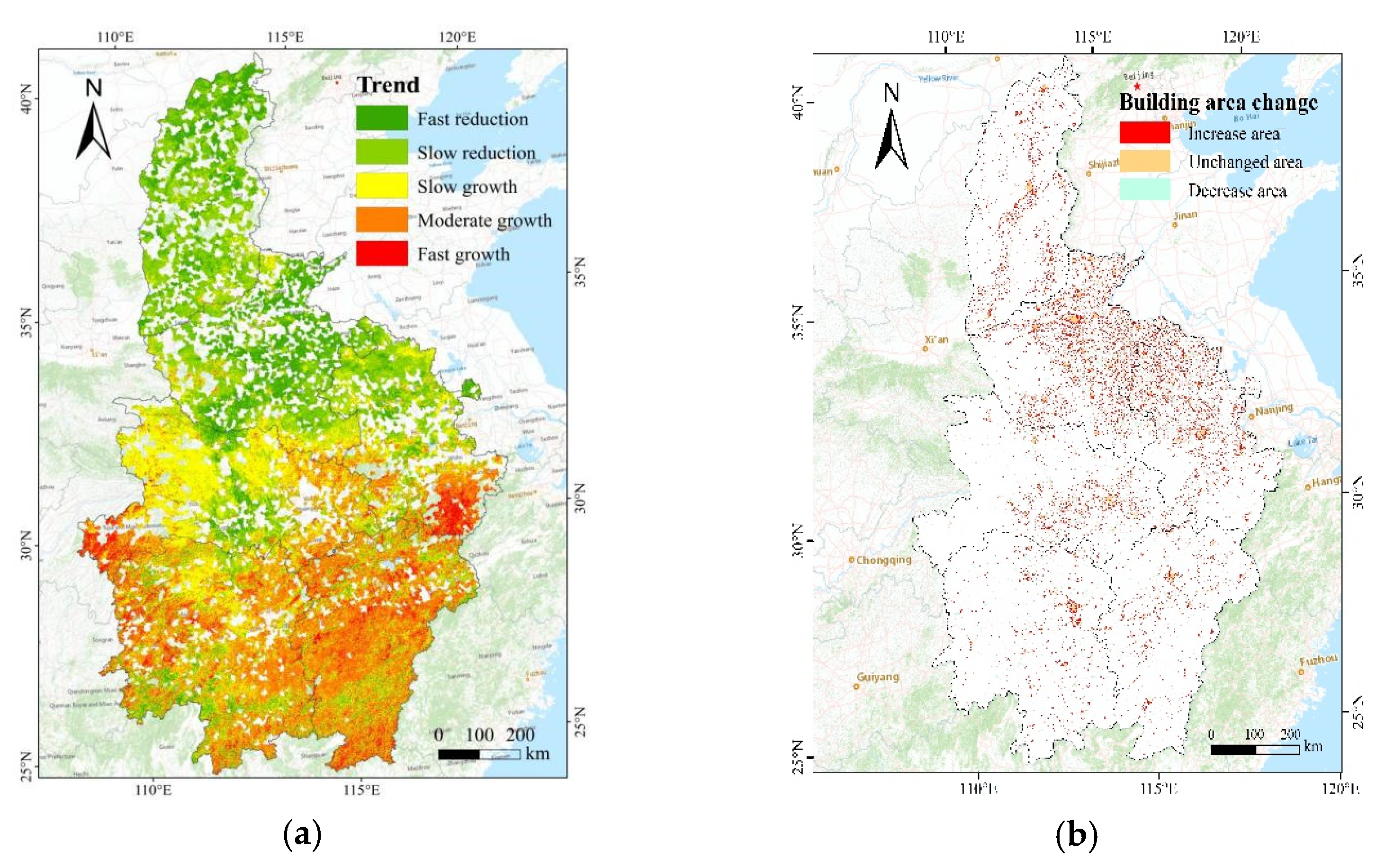
4.1. Identifying the Potential Population Hollowing Regions via Trend Analysis Based on NPP-VIIRS-like Nighttime Lights Images
4.2. The Evaluation and Comparison of Calibration Models for Population Hollowing
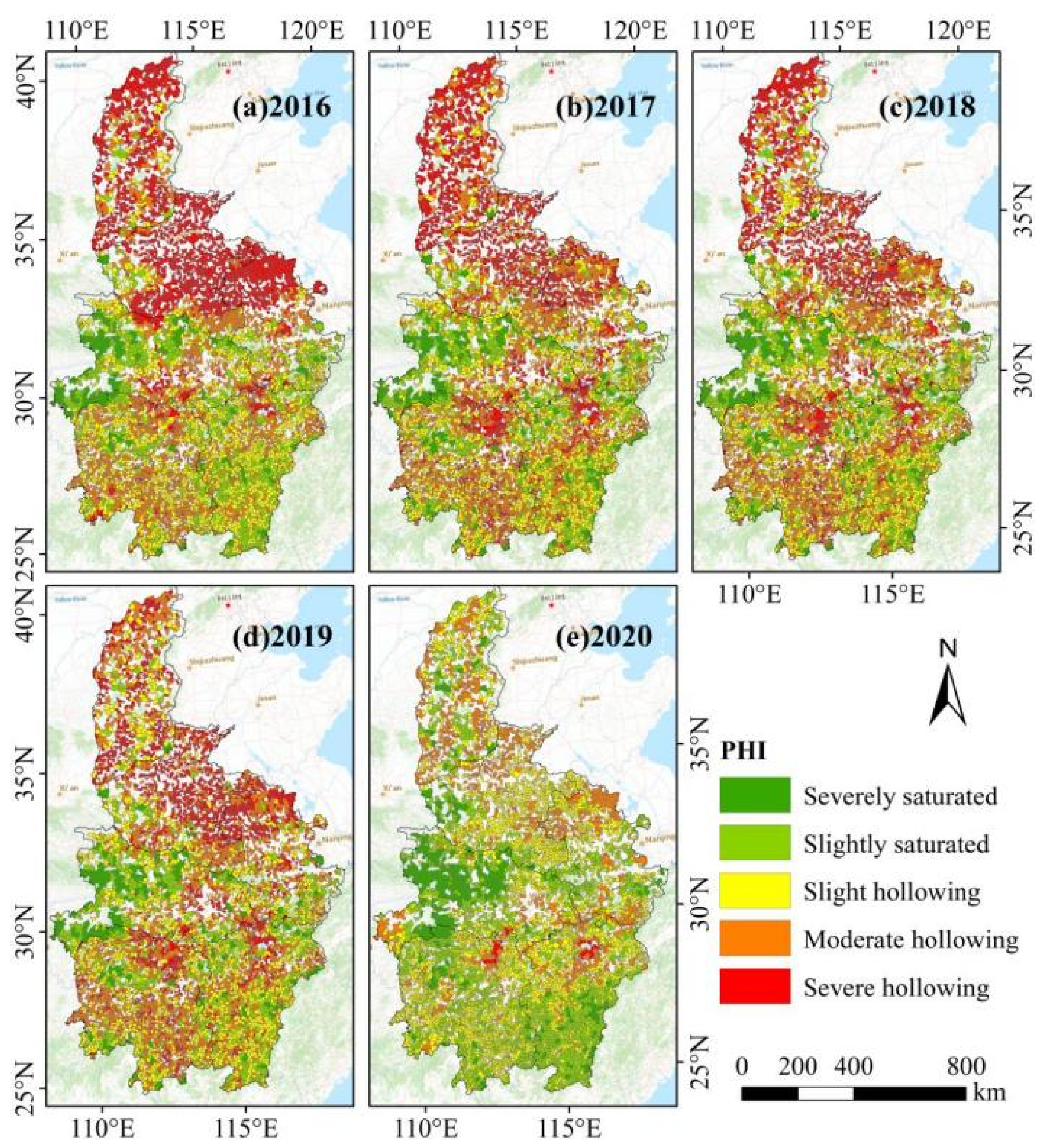
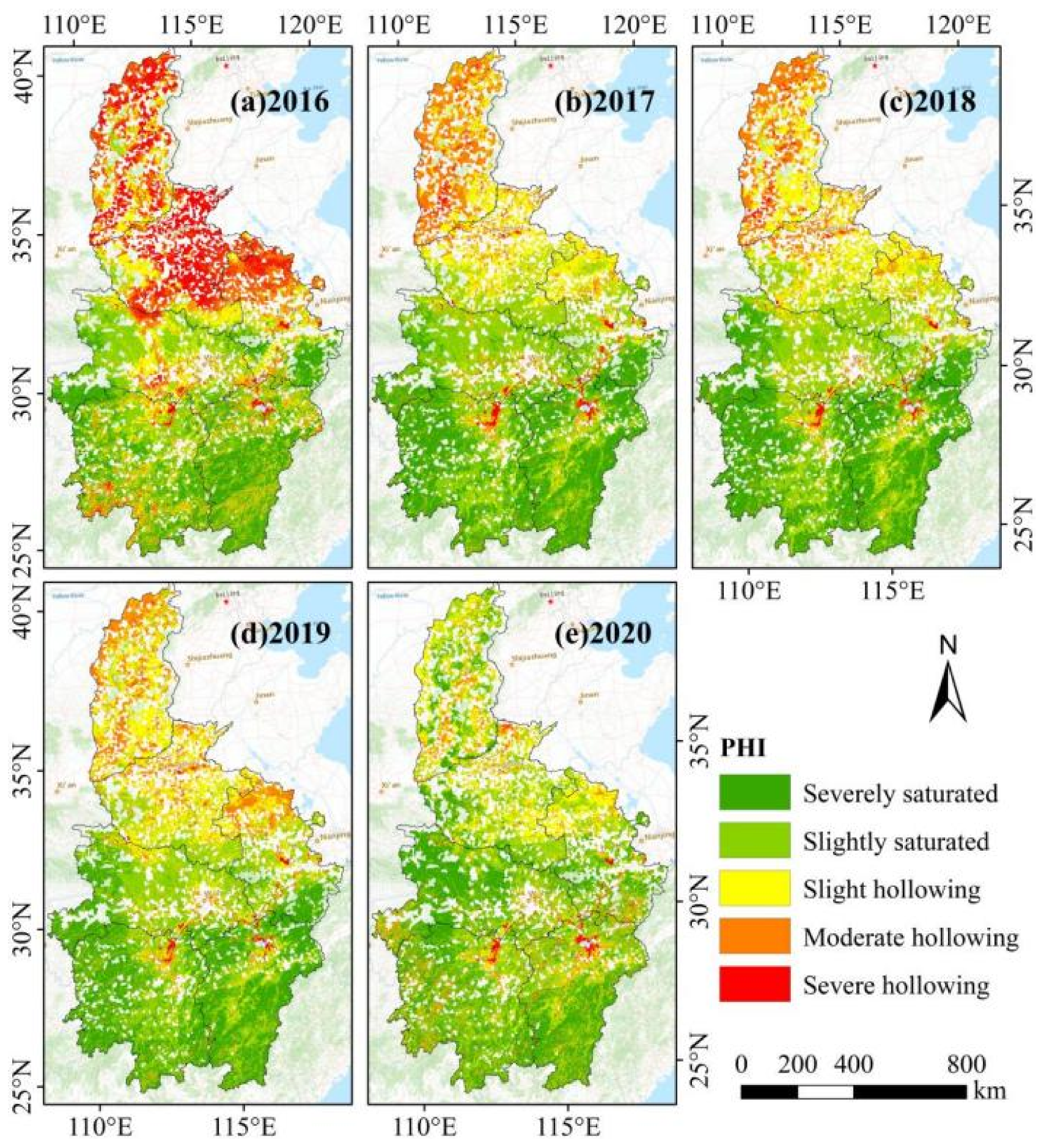
4.3. The Distribution and Spatiotemporal Dynamic Characteristic of Population Hollowing
5. Discussion
5.1. The Comparison between Our Scheme and the Previous Studies
5.2. The Possible Reasons and Explanations for the Distribution and Dynamics of Population Hollowing across the Study Area during 2016–2020
5.3. Limitations of the Current Study
6. Conclusions
Author Contributions
Funding
Institutional Review Board Statement
Informed Consent Statement
Data Availability Statement
Acknowledgments
Conflicts of Interest
References
- Hu, L. Research on Optimal Strategy of Agricultural Products Marketing. J. Innov. Soc. Sci. Res. 2021, 8, 29–33. [Google Scholar] [CrossRef]
- Tan, X. Thinking and Practice of Village Tourism Development Planning under the Strategy of Rural Revitalization—A Case Study of Rural Tourism Development Planning in Dongqiao Village, Wuxi County, Chongqing. Sustain. Dev. 2020, 10, 182–186. [Google Scholar] [CrossRef]
- Ying, L.; Shu, L.; Li, P. The Hollowing Process of Rural Communities in China: Considering the Regional Characteristic. Land 2021, 10, 911. [Google Scholar]
- Liu, Y.; Liu, Y. Geographical research and optimizing practice of rural hollowing in China. Acta Geogr. Sin. 2009, 64, 1193–1202. [Google Scholar]
- Liu, Y.; Liu, Y.; Chen, Y.; Long, H. The process and driving forces of rural hollowing in China under rapid urbanization. J. Geogr. Sci. 2010, 20, 876–888. [Google Scholar] [CrossRef]
- Liu, Y.; Liu, Y. Progress and Prospect on the Study of Rural Hollowing in China. Geogr. Res. 2010, 29, 35–42. [Google Scholar]
- Zhang, W.; Lu, Z.; Yuan, X.; Wang, C.; Gu, Y.; Xu, H.; Streets, D.G. Black carbon emissions from biomass and coal in rural China. Atmos. Environ. 2018, 176, 158–170. [Google Scholar] [CrossRef]
- Long, H. Land consolidation: An indispensable way of spatial restructuring in rural China. J. Geogr. Sci. 2014, 24, 211–225. [Google Scholar] [CrossRef]
- Tang, C.; Hua, H.; Zhou, G.; Zeng, S.; Xiao, L. The research on optimization mode of spatial organization of rural settlements oriented by life quality. Acta Geogr. Sin. 2014, 69, 1459–1472. [Google Scholar]
- Feng, Y.; Ma, J. Rural Ecological Landscape Construction from the Perspective of Rural Revitalization Strategy. J. Landsc. Res. 2018, 10, 135–137. [Google Scholar]
- Liu, Y. Research on the urban-rural integration and rural revitalization in the new era in China. Acta Geogr. Sin. 2018, 73, 637–650. [Google Scholar]
- Zhang, T.; Wang, Y.; Liu, Y.; Zhao, M. Establishing an economic insurance system under a multiple dynamic evolution mechanism after rural hollowing renovation. Resour. Sci. 2016, 38, 799–813. [Google Scholar]
- Guo, B.; Bian, Y.; Zhang, D.; Su, Y.; Wang, X.; Zhang, B.; Wang, Y.; Chen, Q.; Wu, Y.; Luo, P. Estimating Socio-Economic Parameters via Machine Learning Methods Using Luojia1-01 Nighttime Light Remotely Sensed Images at Multiple Scales of China in 2018. IEEE Access 2021, 9, 34352–34365. [Google Scholar] [CrossRef]
- Liang, H.; Guo, Z.; Wu, J.; Chen, Z. GDP spatialization in Ningbo City based on NPP/VIIRS night-time light and auxiliary data using random forest regression. Adv. Space Res. 2020, 65, 481–493. [Google Scholar] [CrossRef]
- Zhu, X.; Li, Q.; Shen, M.; Chen, J.; Wu, J. A methodology for multiple cropping index extraction based on NDVI time-series. Nat. Resour 2008, 23, 534–544. [Google Scholar]
- Guo, B.; Zhang, D.; Zhang, D.; Su, Y.; Wang, X.; Bian, Y. Detecting spatiotemporal dynamic of regional electric consumption using NPP-VIIRS nighttime stable light data—A case study of Xi’an, China. IEEE Access 2020, 8, 171694–171702. [Google Scholar] [CrossRef]
- Wang, C.; Chen, Z.; Yang, C.; Li, Q.; Wu, Q.; Wu, J.; Zhang, G.; Yu, B. Analyzing parcel-level relationships between Luojia 1-01 nighttime light intensity and artificial surface features across Shanghai, China: A comparison with NPP-VIIRS data. Int. J. Appl. Earth Obs. Geoinf. 2020, 85, 101989. [Google Scholar] [CrossRef]
- Niu, T.; Chen, Y.; Yuan, Y. Measuring urban poverty using multi-source data and a random forest algorithm: A case study in Guangzhou. Sustain. Cities Soc. 2020, 54, 102014. [Google Scholar] [CrossRef]
- Zhang, F.; Zhang, D.; Liu, Y.; Lin, H. Representing place locales using scene elements. Computers. Environ. Urban Syst. 2018, 71, 153–164. [Google Scholar] [CrossRef]
- Joshua, B.; Gabriel, C.; Robert, O. Predicting poverty and wealth from mobile phone metadata. Science 2015, 350, 1073–1076. [Google Scholar]
- Long, Y.; Shen, Z. Geospatial Analysis to Support Urban Planning in Beijing; Springer: Cham, Switzerland, 2015; Volume 116, pp. 1–272. [Google Scholar]
- Hu, L.; He, S.; Han, Z.; Xiao, H.; Su, S.; Weng, M.; Cai, Z. Monitoring housing rental prices based on social media: An integrated approach of machine-learning algorithms and hedonic modeling to inform equitable housing policies. Land Use Policy 2019, 82, 657–673. [Google Scholar] [CrossRef]
- Ye, T.; Zhao, N.; Yang, X.; Ouyang, Z.; Liu, X.; Chen, Q.; Hu, K.; Yue, W.; Qi, J.; Li, Z.; et al. Improved population mapping for China using remotely sensed and points-of-interest data within a random forests model. Sci. Total Environ. 2019, 658, 936–946. [Google Scholar] [CrossRef] [PubMed]
- Levin, N.; Duke, Y. High spatial resolution night-time light images for demographic and socio-economic studies. Remote Sens. Environ. 2012, 119, 1–10. [Google Scholar] [CrossRef]
- Yu, B.L.; Lian, T.; Huang, Y.X.; Yao, S.J.; Ye, X.Y.; Chen, Z.Q.; Yang, C.S.; Wu, J.P. Integration of nighttime light remote sensing images and taxi GPS tracking data for population surface enhancement. Int. J. Geogr. Inf. Sci. 2019, 33, 687–706. [Google Scholar] [CrossRef]
- Zhang, Y.; Li, Y.; Chen, Y.; Liu, S.; Yang, Q. Spatiotemporal Heterogeneity of Urban Land Expansion and Urban Population Growth under New Urbanization: A Case Study of Chongqing. Int. J. Environ. Res. Public Health 2022, 19, 7792. [Google Scholar] [CrossRef] [PubMed]
- Liu, J.; Zhang, X.; Lin, J.; Li, Y. Beyond government-led or community-based: Exploring the governance structure and operating models for reconstructing China’s hollowed villages. J. Rural Stud. 2022, 93, 273–286. [Google Scholar] [CrossRef]
- Hu, T.; Wang, T.; Yan, Q.Y.; Chen, T.X.; Jin, S.G.; Hu, J. Modeling the spatiotemporal dynamics of global electric power consumption (1992–2019) by utilizing consistent nighttime light data from DMSP-OLS and NPP-VIIRS. Appl. Energy 2022, 322, 119473. [Google Scholar] [CrossRef]
- Lu, L.; Weng, Q.; Xie, Y.; Guo, H.; Li, Q. An assessment of global electric power consumption using the Defense Meteorological Satellite Program-Operational Linescan System nighttime light imagery. Energy 2019, 189, 116351. [Google Scholar] [CrossRef]
- Jiang, L.G.; Liu, Y.; Wu, S.; Yang, C. Study on Urban Spatial Pattern Based on DMSP/OLS and NPP/VIIRS in Democratic People’s Republic of Korea. Remote Sens. 2021, 13, 4879. [Google Scholar] [CrossRef]
- Mills, G.; Pleijel, H.; Malley, C.S.; Sinha, B.; Cooper, O.R.; Schultz, M.G.; Neufeld, H.S.; Simpson, D.; Sharps, K.; Feng, Z.; et al. Tropospheric Ozone Assessment Report: Present-day tropospheric ozone distribution and trends relevant to vegetation. Elem. Sci. Anth. 2018, 6, 47. [Google Scholar] [CrossRef]
- Zhao, N.; Liu, Y.; Cao, G.; Samson, E.L.; Zhang, J. Forecasting China’s GDP at the pixel level using nighttime lights time series and population images. GIScience Remote Sens. 2017, 54, 407–425. [Google Scholar] [CrossRef]
- Shi, K.; Chang, Z.; Chen, Z.; Wu, J.; Yu, B. Identifying and evaluating poverty using multisource remote sensing and point of interest (POI) data: A case study of Chongqing, China. J. Clean. Prod. 2020, 255, 120245. [Google Scholar] [CrossRef]
- Ingacheva, A.; Kokhan, V. Mapping China’s ghost cities through the combination of nighttime satellite data and daytime satellite data. In Proceedings of the 32nd European Conference on Modelling and Simulation (ECMS), Wilhelmshaven, Germany, 22–25 May 2018. [Google Scholar]
- Cheng, L.; Feng, W.Y.; Jiang, L.H. The Analysis of Rural Settlement Hollowizing System of the Southeast of Taiyuan Basin. Acta Geogr. Sin. 2001, 56, 437–446. [Google Scholar]
- Long, H.; Li, Y.R.; Liu, Y.S. Analysis of Evolutive Characteristics and Their Driving Mechanism of Hollowing Villages in China. Acta Geogr. Sin. 2009, 64, 1203–1213. [Google Scholar]
- Jie, Y.W.; Yan, S.L.; Yang, F.C. Empirical analysis on influencing factors of the hollowing village degree: Based on the survey data of sample villages in Shandong province. J. Nat. Resour. 2013, 28, 10–18. [Google Scholar]
- Song, W.; Chen, B.M.; Zhang, Y. Typical survey and analysis on influencing factors of village-hollowing of rural housing land in China. Geogr. Res. 2013, 32, 20–28. [Google Scholar]
- Yu, Z.; Xiao, L.; Chen, X.; He, Z.; Guo, Q.; Vejre, H. Spatial restructuring and land consolidation of urban-rural settlement in mountainous areas based on ecological niche perspective. J. Geogr. Sci. 2018, 28, 131–151. [Google Scholar] [CrossRef] [Green Version]
- Chung, S.H. Population Change and Risk of Regional Extinction in Gangwon Province. J. Soc. Sci. 2019, 58, 3–22. [Google Scholar] [CrossRef]
- Liu, S.; Bai, M.; Yao, M.; Huang, K. Identifying the natural and anthropogenic factors influencing the spatial disparity of population hollowing in traditional villages within a prefecture-level city. PLoS ONE 2021, 16, 4. [Google Scholar] [CrossRef]
- Lee, J.; Suh, K. A New Index to Assess Vulnerability to Regional Shrinkage (Hollowing out) Due to the Changing Age Structure and Population Density. Sustainability 2021, 13, 9382. [Google Scholar] [CrossRef]
- Tan, X.; Yu, S.Y.; Ouyang, Q.L.; Mao, K.B.; He, Y.H.; Zhou, G.H. Assessment and influencing factors of rural hollowing in the rapid urbanization region: A case study of Chang sha-Zhuzhou-Xiangtan urban agglomeration. Geogr. Res. 2017, 36, 684–694. [Google Scholar]
- Leng, B.-B.; Le, X.-L.; Yuan, G.; Ji, X.-Q. The economic support index evaluation study on the pig breeding scale of the six provinces in central China. IOP Conf. Ser. Earth Environ. Sci. 2017, 94, 12053. [Google Scholar] [CrossRef] [Green Version]
- Wang, Z.; Zhang, F.; Wu, F. Intergroup neighbouring in urban China: Implications for the social integration of migrants. Urban Stud. 2016, 53, 651–668. [Google Scholar] [CrossRef]
- Leng, B.; Ji, X.; Huang, L. Evaluation research on natural resource supply index of the pig breeding scale in the six provinces of central China. IOP Conf. Ser. Earth Environ. Sci. 2017, 81, 12106. [Google Scholar] [CrossRef] [Green Version]
- Qiu, L.; Xiao, H. Notice of retraction a feasibility study on the service economy in the rise of central China. In Proceedings of the 2009 International Conference on Management and Service Science, Wuhan/Beijing, China, 20–22 September 2009. [Google Scholar]
- Chen, Z.; Yu, B.; Yang, C.; Zhou, Y.; Yao, S.; Qian, X.; Wang, C.; Wu, B.; Wu, J. An Extended TimeSeries (2000–2018) of Global NPP-VIIRS-like Nighttime Light Data from a Cross-Sensor Calibration. Earth Syst. Sci. Data 2021, 13, 889–906. [Google Scholar] [CrossRef]
- Liu, H.; Liu, X. Establishment of a New Spatial Agglomeration of an Open Economy: Theoretical Basis, Historical Practice and Feasible Pathways. Contemp. Soc. Sci. 2020, 4, P1–P24. [Google Scholar]
- Guo, B.; Zhang, D.; Pei, L.; Su, Y.; Wang, X.; Bian, Y.; Zhang, D.; Yao, W.; Zhou, Z.; Guo, L. Estimating PM2.5 Concentrations via Random Forest Method Using Satellite, Auxiliary, and Ground-level Station Dataset at Multiple Temporal Scales across China in 2017. Sci. Total Environ. 2021, 778, 146288. [Google Scholar] [CrossRef]
- Zhang, G.; Guo, X.; Li, D.; Jiang, B. Evaluating the Potential of LJ1-01 Nighttime Light Data for Modeling Socio-Economic Parameters. Sensors. 2019, 19, 1465. [Google Scholar] [CrossRef] [Green Version]
- Wang, Y.; Guo, B.; Pei, L.; Guo, H.J.; Zhang, D.M.; Ma, X.Y.; Yu, Y.; Wu, H.J. The influence of socioeconomic and environmental determinants on acute myocardial infarction (AMI) mortality from the spatial epidemiological perspective. Environ. Sci. Pollut. Res. 2022, 1–18. [Google Scholar] [CrossRef]
- Guo, B.; Wang, X.; Zhang, D.; Pei, L.; Zhang, D.; Wang, X. A land use regression application into simulating spatial distribution characteristics of particulate matter (PM2.5) concentration in city of Xi’an, China. Pol. J. Environ. Stud. 2020, 29, 4065–4076. [Google Scholar] [CrossRef]
- Sun, X. Green city and regional environmental economic evaluation based on entropy method and GIS. Environ. Technol. Innov. 2021, 23, 101667. [Google Scholar] [CrossRef]
- Xue, J.; Shi, L.; Wang, H.; Ji, Z.; Shang, H.; Xu, F.; Zhao, C.; Huang, H.; Luo, A. Water abundance evaluation of a burnt rock aquifer using the AHP and entropy weight method: A case study in the Yongxin coal mine, China. Environ. Earth Sci. 2021, 80, 417. [Google Scholar] [CrossRef]
- Hu, Y.; Wu, X. Research on Spatial Differentiation and Influencing Factors of Hollowing Rural Population in Anhui Province. J. Yunnan Agric. Univ. (Soc. Sci.) 2020, 14, 25–31. (In Chinese) [Google Scholar]
- Yin, D.; Gui, J.; Xiangzheng, D.; Feng, W. Multidimensional measurement of poverty and its spatio-temporal dynamics in China from the perspective of development geography. J. Geogr. Sci. 2021, 31, 130–148. [Google Scholar]
- Guo, B.; Wang, Y.; Pei, L.; Yu, Y.; Liu, F.; Zhang, D.; Wang, X.; Su, Y.; Zhang, D.; Zhang, B.; et al. Determining the effects of socioeconomic and environmental determinants on chronic obstructive pulmonary disease (COPD) mortality using geographically and temporally weighted regression model across Xi’an during 2014–2016. Sci. Total Environ. 2021, 756, 143869. [Google Scholar] [CrossRef] [PubMed]
- Song, W.; Jia, H.; Huang, J.; Zhang, Y. A satellite-based geographically weighted regression model for regional PM2.5 estimation over the Pearl River Delta region in China. Remote Sens. Environ. 2014, 154, 1–7. [Google Scholar] [CrossRef]
- Pei, L.; Wang, X.; Guo, B.; Guo, H.; Yu, Y. Do air pollutants as well as meteorological factors impact Corona Virus Disease 2019 (COVID-19)? Evidence from China based on the geographical perspective. Environ. Sci. Pollut. Res. 2021, 28, 35584–35596. [Google Scholar] [CrossRef]
- He, Q.; Huang, B. Satellite-based mapping of daily high-resolution ground PM2.5 in China via space-time regression modeling. Remote Sens. Environ. 2018, 206, 72–83. [Google Scholar] [CrossRef]
- Steininger, M.; Defries, R.; Belward, A. Satellite estimation of tropical secondary forest above-ground biomass: Data from Brazil and Bolivia. Int. J. Remote Sens. 2000, 21, 1139–1157. [Google Scholar] [CrossRef]
- Zhang, B.; Guo, B.; Zou, B.; Wei, W.; Lei, Y.Z.; Li, T.Q. Retrieving soil heavy metals concentrations based on GaoFen-5 hyperspectral satellite image at an opencast coal mine, Inner Mongolia, China. Environ. Pollut. 2022, 300, 118981. [Google Scholar] [CrossRef]
- Guo, B.; Zhang, B.; Su, Y.; Zhang, D.; Wang, Y.; Bian, Y.; Suo, L.; Guo, X.; Bai, H. Retrieving zinc concentrations in topsoil with reflectance spectroscopy at Opencast Coal Mine sites. Sci. Rep. 2021, 11, 19909. [Google Scholar] [CrossRef] [PubMed]
- Breiman, L. Random Forests. Mach. Learn 2001, 45, 5–32. [Google Scholar]
- Zheng, D.; Rademacher, J.; Chen, J.; Crow, T.; Bresee, M.; Moine, J.L.; Ryu, S. Estimating aboveground biomass using Landsat 7 ETM+ data across a managed landscape in northern Wisconsin, USA. Remote Sens. Environ. 2004, 93, 402–411. [Google Scholar] [CrossRef]
- Ham, J.; Chen, Y.; Crawford, M.M.; Ghosh, J. Investigation of the random forest framework for classification of hyperspectral data. IEEE Trans. Geosci. Remote Sens. 2005, 43, 492–501. [Google Scholar] [CrossRef] [Green Version]
- Wei, J.; Li, Z.; Cribb, M.; Huang, W.; Xue, W.; Sun, L.; Guo, J.; Peng, Y.; Li, J.; Lyapustin, A.; et al. Improved 1 km resolution PM. estimates across China using enhanced space-time extremely randomized trees. Atmos. Chem. Phys. 2020, 20, 3273–3289. [Google Scholar] [CrossRef] [Green Version]
- Xu, Z. Influencing Factors and Urbanization Effects of the Spatial Pattern of Floating Population in Anhui Province. J. Landsc. Res. 2019, 11, 88–98. [Google Scholar]
- Dotto, A.; Dalmolin, R.; Ten Caten, A.; Grunwald, S. A systematic study on the application of scatter-corrective and spectral-derivative preprocessing for multivariate prediction of soil organic carbon by Vis-NIR spectra. Geoderma 2018, 314, 262–274. [Google Scholar] [CrossRef]
- Guo, B.; Wang, X.; Pei, L.; Su, Y.; Zhang, D.; Wang, Y. Identifying the spatiotemporal dynamic of PM2.5 concentrations at multiple scales using geographically and temporally weighted regression model across China during 2015–2018. Sci. Total Environ. 2021, 751, 141765. [Google Scholar] [CrossRef]
- Guo, B.; Su, Y.; Pei, L.; Wang, X.; Zhang, B.; Zhang, D.; Wang, X. Ecological risk evaluation and source apportionment of heavy metals in park playgrounds: A case study in Xi’an, Shaanxi Province, a northwest city of China. Environ. Sci. Pollut. R 2020, 27, 24400–24412. [Google Scholar] [CrossRef]
- Guo, B.; Su, Y.; Pei, L.; Wang, X.; Wei, X.; Zhang, B.; Zhang, D.; Wang, X. Contamination, Distribution and Health Risk Assessment of Risk Elements in Topsoil forAmusement Parks in Xi’an, China. Pol. J. Environ. Stud. 2021, 30, 601–617. [Google Scholar] [CrossRef]
- Liang, X.; Tang, X.; Luo, Y.; Zhang, M.; Feng, Z. Effects of policies and containment measures on control of COVID-19 epidemic in Chongqing. World J. Clin. Cases 2020, 8, 2959–2976. [Google Scholar] [CrossRef] [PubMed]
- Hong, Y.; Shen, R.; Cheng, H.; Chen, Y.; Zhang, Y.; Liu, Y.; Zhou, M.; Yu, L.; Liu, Y.; Liu, Y. Estimating lead and zinc concentrations in peri-urban agricultural soils through reflflectance spectroscopy: Effects of fractional-order derivative and random forest. Sci. Total Environ. 2019, 651, 1969–1982. [Google Scholar] [CrossRef]
- Wei, J.; Huang, W.; Li, Z.; Xue, W.; Peng, Y.; Sun, L.; Cribb, M. Estimating 1-kmresolution PM2.5 concentrations across China using the space-time random forest approach. Remote Sens. Environ. 2019, 231, 111221. [Google Scholar] [CrossRef]
- Lan, Z.; Chun, Y. Beautiful Village Planning and Construction: A Practice of Human Settlement Improvement in Jiangsu Province. China City Plan. Rev. 2014, 23, 40–50. [Google Scholar]
- Peng, J.; Chen, S.; Lü, H.; Liu, Y.; Wu, J. Spatiotemporal patterns of remotelysensed PM2.5 concentrations in China from 1999 to 2011. Remote Sens. Environ. 2016, 174, 109–121. [Google Scholar] [CrossRef]
- Xie, H.; Zou, J.; Peng, X. Spatial-temporal difference analysis of cultivated land use intensity based on emergy in Poyang Lake eco-economic zone. ActaGeograph. Sin. 2012, 67, 889–902. [Google Scholar]
- Rodríguez-Puerta, F.; Alonso Ponce, R.; Pérez-Rodríguez, F.; Águeda, B.; Martín-García, S.; Martínez-Rodrigo, R.; Lizarralde, I. Comparison of Machine Learning Algorithms for Wildland-Urban Interface Fuelbreak Planning Integrating ALS and UAV-Borne LiDAR Data and Multispectral Images. Drones 2020, 4, 21. [Google Scholar] [CrossRef]
- Ganggayah, M.; Taib, N.; Har, Y.; Lio, P.; Dhillon, S. Predicting factors for survival of breast cancer patients using machine learning techniques. BioMed. Cent. 2019, 19, 48. [Google Scholar] [CrossRef] [Green Version]
- Qi, W.; Yi, J. Spatial pattern and driving factors of migrants on the Qinghai-Tibet Plateau: Insights from short-distance and long-distance population migrants. J. Geogr. Sci. 2021, 31, 215–230. [Google Scholar] [CrossRef]
- En, W.; Xue, B.; Yang, J.; Lu, C. Effects of the Northeast China Revitalization Strategy on Regional Economic Growth and Social Development. Chin. Geogr. Sci. 2020, 30, 791–809. [Google Scholar]
- Wu, Q.; Chen, J. The Effect and Influence of Tourism Poverty Alleviation of Residents in Poor Areas: A Case Study of Key Tourism Poverty Alleviation Villages in Northern Guangdong. J. Landsc. Res. 2021, 13, 89–94. [Google Scholar]
- Ye, Y.; Wang, C.; Zhang, H.; Yang, J.; Liu, Z.; Wu, K.; Deng, Y. Spatiotemporal analysis of COVID-19 risk in Guangdong Province based on population migration. J. Geogr. Sci. 2020, 30, 1985–2001. [Google Scholar] [CrossRef]
- Yin, Y.; Zhang, Y. Environmental Pollution Evaluation of Urban Rail Transit Construction Based on Entropy Weight Method. Nat. Environ. Pollut. Technol. 2021, 20, 819–824. [Google Scholar] [CrossRef]
- Wang, X.; Li, Y.; Li, Y.; Chen, Y.; Lian, J.; Cao, W. Comparison of sampling schemes for spatial prediction of soil organic carbon in Northern China. Sci. Cold Arid Reg. 2020, 12, 200–216. [Google Scholar]
- Xu, P.; Lin, M.; Jin, P. Spatio-temporal Dynamics of Urbanization in China Using DMSP/OLS Nighttime Light Data from 1992–2013. Chin. Geogr. Sci. 2021, 31, 70–80. [Google Scholar] [CrossRef]
- Zhao, F.; Ding, J.; Zhang, S.; Luan, G.; Song, L.; Peng, Z.; Du, Q.; Xie, Z. Estimating Rural Electric Power Consumption Using NPP-VIIRS Night-Time Light, Toponym and POI Data in Ethnic Minority Areas of China. Remote Sens. 2020, 12, 2836. [Google Scholar] [CrossRef]
- Shi, K.; Yu, B.; Huang, C.; Wu, J.; Sun, X. Exploring spatiotemporal patterns of electric power consumption in countries along the Belt and Road. Energy 2018, 150, 847–859. [Google Scholar] [CrossRef]


| Sorts | Factors | Sources | Resolution |
|---|---|---|---|
| Physical geography | DEM | http://www.gscloud.cn/ (accessed on 1 January 2021). | 2015 (30 m) |
| Waterbody density (WD) | http://www.openstreetmap.org/ (accessed on 1 January 2021). | 2016–2020 (Vector data) | |
| Meteorological factors concerning Atmospheric pressure (PRS), Relative humidity (RHU), Temperature (TEM), Wind speed (WIN), Precipitation (PRE) | http://data.cma.cn/ (accessed on 1 January 2021). | 2016–2020 (Monthly ground-level monitoring station data) | |
| NDVI | https://modis.gsfc.nasa.gov/ (accessed on 1 January 2021). | 2016–2020 (250 m) | |
| Human geography | Point of interest (POI) | http://www.openstreetmap.org/ (accessed on 1 January 2021). | 2016–2020 (Vector data) |
| Road density (RD) | |||
| GDP | Statistical yearbook, The statistical report, the official website of each regional statistical bureau, Census report | 2016–2020 (township) | |
| Population Statistical data | |||
| Related agricultural data | |||
| Population density (POP) | https://www.worldpop.org/ (accessed on 1 January 2021). | 2016–2020 (1000 m) | |
| NPP-VIIRS Monthly nighttime stable light (NTL) composite data | https://ngdc.noaa.gov/ (accessed on 1 January 2021). | 2016–2020 (742 m) | |
| Global NPP-VIIRS-like nighttime light data | http://doi.org/10.7910/DVN/YGIVCD (accessed on 1 January 2021). | 2000–2015 (15 arc seconds) | |
| Air Pollutants (CO, NO2, O3, PM10, PM2.5, SO2) | http://www.cnemc.cn/ (accessed on 1 January 2021). | 2016–2020 (Hourly ground-level monitoring station data) |
| Indicators | Weights | Effects | Calculation Methods |
|---|---|---|---|
| Population outflow rate | 0.21 | positive | (Registered population–permanent population)/Registered population |
| The ratio of 0–14 years old to the total population | 0.18 | positive | 0–14 years population/Total population |
| The ratio of the over 65 population to the total population | 0.18 | positive | Population over 65/Total population |
| The ratio of rural permanent population to the total rural population | 0.17 | negative | Rural permanent population/Total rural population |
| The ratio of the rural employed population to the total rural population | 0.15 | negative | Rural employees/Total rural population |
| Average agricultural land | 0.11 | positive | Total agricultural land area/Total rural population |
| The Total Number of Townships | The Number of Townships with Slope1 > 0 | The Number of Townships Slope1 > 0 and p ≤ 0.05 | The Number of Townships with Slope1 ≤ 0 | The Number of Potential Population Hollowing Townships |
|---|---|---|---|---|
| 9254 | 4864 | 2512 | 4390 | 6742 |
| 2016 | 2017 | 2018 | 2019 | 2020 | ||||||
|---|---|---|---|---|---|---|---|---|---|---|
| RF | C | V | C | V | C | V | C | V | C | V |
| R2 | 0.6076 | 0.5882 | 0.6125 | 0.6033 | 0.6087 | 0.5898 | 0.6246 | 0.6061 | 0.6235 | 0.5877 |
| RMSE | 0.0301 | 0.0462 | 0.0216 | 0.0351 | 0.0214 | 0.0311 | 0.0297 | 0.0477 | 0.0295 | 0.0501 |
| MAE | 0.0248 | 0.0371 | 0.0167 | 0.0302 | 0.0116 | 0.0251 | 0.0245 | 0.0403 | 0.0244 | 0.0461 |
| GWR | C | V | C | V | C | V | C | V | C | V |
| R2 | 0.4291 | 0.3769 | 0.4425 | 0.3986 | 0.4064 | 0.3751 | 0.4343 | 0.4012 | 0.4289 | 0.3784 |
| RMSE | 0.0763 | 0.0801 | 0.0772 | 0.0869 | 0.0796 | 0.0907 | 0.0737 | 0.0799 | 0.0759 | 0.0844 |
| MAE | 0.0681 | 0.0749 | 0.0657 | 0.0705 | 0.0699 | 0.0762 | 0.0676 | 0.0708 | 0.0687 | 0.0738 |
| MLR | C | V | C | V | C | V | C | V | C | V |
| R2 | 0.1022 | 0.0917 | 0.1276 | 0.0619 | 0.0954 | 0.0776 | 0.0879 | 0.0691 | 0.1075 | 0.0641 |
| RMSE | 0.0997 | 0.1864 | 0.0912 | 0.1859 | 0.1033 | 1.1793 | 0.1268 | 0.1854 | 0.0955 | 0.1845 |
| MAE | 0.0779 | 0.1254 | 0.0736 | 0.1304 | 0.0802 | 0.1289 | 0.0839 | 0.1201 | 0.0725 | 0.1293 |
Publisher’s Note: MDPI stays neutral with regard to jurisdictional claims in published maps and institutional affiliations. |
© 2022 by the authors. Licensee MDPI, Basel, Switzerland. This article is an open access article distributed under the terms and conditions of the Creative Commons Attribution (CC BY) license (https://creativecommons.org/licenses/by/4.0/).
Share and Cite
Guo, B.; Bian, Y.; Pei, L.; Zhu, X.; Zhang, D.; Zhang, W.; Guo, X.; Chen, Q. Identifying Population Hollowing Out Regions and Their Dynamic Characteristics across Central China. Sustainability 2022, 14, 9815. https://doi.org/10.3390/su14169815
Guo B, Bian Y, Pei L, Zhu X, Zhang D, Zhang W, Guo X, Chen Q. Identifying Population Hollowing Out Regions and Their Dynamic Characteristics across Central China. Sustainability. 2022; 14(16):9815. https://doi.org/10.3390/su14169815
Chicago/Turabian StyleGuo, Bin, Yi Bian, Lin Pei, Xiaowei Zhu, Dingming Zhang, Wencai Zhang, Xianan Guo, and Qiuji Chen. 2022. "Identifying Population Hollowing Out Regions and Their Dynamic Characteristics across Central China" Sustainability 14, no. 16: 9815. https://doi.org/10.3390/su14169815
APA StyleGuo, B., Bian, Y., Pei, L., Zhu, X., Zhang, D., Zhang, W., Guo, X., & Chen, Q. (2022). Identifying Population Hollowing Out Regions and Their Dynamic Characteristics across Central China. Sustainability, 14(16), 9815. https://doi.org/10.3390/su14169815