Article

Spatial Variations of Village-Level Environmental Variables from Satellite Big Data and Implications for Public Health–Related Sustainable Development Goals

1
Center for Geographic Analysis, Harvard University, Cambridge, MA 02138, USA
2
Division of Health Policy and Management, College of Health Science, Korea University, Seoul 02841, Korea
3
Interdisciplinary Program in Precision Public Health, Department of Public Health Sciences, Graduate School of Korea University, Seoul 02841, Korea
4
Harvard Center for Population and Development Studies, Cambridge, MA 02138, USA
5
Department of Social and Behavioral Sciences, Harvard T.H. Chan School of Public Health, Boston, MA 02115, USA
*
Author to whom correspondence should be addressed.
Sustainability 2022, 14(16), 10450; https://doi.org/10.3390/su141610450
Submission received: 4 June 2022 / Revised: 28 July 2022 / Accepted: 29 July 2022 / Published: 22 August 2022

Abstract

:
The United Nations Sustainable Development Goals (SDGs) include 17 interlinked goals designed to be a blueprint for the world’s nations to achieve a better and more sustainable future, and the specific SDG 3 is a public health–related goal to ensure healthy living and promote well-being for all population groups. To facilitate SDG planning, implementation, and progress monitoring, many SDG indicators have been developed. Based on the United Nations General Assembly resolutions, SDG indicators need to be disaggregated by geographic locations and thematic environmental and socioeconomic characteristics for achieving the most accurate planning and progress assessment. High-resolution data such as those captured at the village level can provide comparatively more precise insights into the different socioeconomic and environmental factors relevant to SDGs, therefore enabling more effective sustainable development decision-making. Using India as our study area and the child malnutrition indicators stunting, underweight, and wasting as examples of public health–related SDG indicators, we have demonstrated a process to effectively derive environmental variables at the village level from satellite big datasets on a cloud platform for SDG research and applications. Spatial analysis of environmental variables regarding vegetation, climate, and terrain have shown spatial grouping patterns across the entire study area, with each village group having different statistics. Correlation analysis between these environmental variables and stunting, underweight, and wasting indicators show a meaningful relationship between these indicators and vegetation index, land surface temperature, rainfall, elevation, and slope. Identifying the spatial variation patterns of environmental variables at the village level and their correlations with child malnutrition indicators can be an invaluable tool to facilitate a clearer understanding of the causes of child malnutrition and to improve area-specific SDG 3 implementation planning. This analysis can also provide meaningful support in assessing and monitoring SDG implementation progress at the village level by spatially predicting SDG indicators using available socioeconomic and environmental independent variables. The methodology used in this study has the potential to be applied to other similar regions, especially low-to-middle income countries where a high number of children are severely affected by malnutrition, as well as to other environmentally related SDGs, such as Goal 1 (No Poverty) and Goal 2 (Zero Hunger).

1. Introduction

The United Nations Sustainable Development Goals (SDGs), set up in 2015 with a target deadline of 2030, include 17 interlinked goals designed to be a blueprint framework for the world’s nations to achieve a better and more sustainable future [1]. Among these goals, the specific SDG 3 is a public health–related goal “to ensure healthy lives and promote well-being for all at all ages”. The United Nations Global Indicator Framework has been developed to facilitate countries in the three SDG implementation phases: planning, implementation, and progress monitoring. Based on the Fundamental Principles of Official Statistics from the United Nations General Assembly resolutions, SDG indicators should be disaggregated by geographic locations and thematic environmental and socioeconomic characteristics in order to achieve the most accurate planning and progress assessment [2].
Geospatial data, including data collected by Earth observation satellites, are among the most important types of data for supporting the three SDG implementation phases [3,4,5]. Village-level data represents the highest resolution of all levels of administration and can provide more specific details about the different socioeconomic and environmental factors affecting SDGs, thus enabling more precise sustainable development decision making [6,7,8,9,10,11,12,13,14]. While village-level socioeconomic data such as census-based demographics are available for some nations, important environmental variables, including vegetation, climate, and terrain, are not yet readily available at such a fine-grained level, hindering sustainable development research and applications [6]. Earth observation satellites collect environmental data with geographic locations referenced, providing the most valuable geospatial datasets about environmental factors for the SDGs [15,16,17,18,19,20,21,22,23]. In addition, the questions of how environmental variables differ spatially at the village level, and whether such variations correlate with SDG indicators, have not yet been reported in the literature.
Focusing on three child malnutrition indicators in India (stunting, underweight, and wasting), this study developed a process to derive village-level environmental variables from a large volume of satellite images, analyzed their spatial variations and relationships with the SDG indicators, and discussed the implications for relevant SDG planning and progress assessment.

2. Materials and Methods

2.1. Study Area

India is the second most populous country in the world as well as one of the largest developing countries. Based on the SDG Index and Dashboard global report 2017, India was ranked No. 110 and 116 out of 157 nations in 2016 and 2017, respectively, for progress on SDGs [3], spotlighting a critical need for improvement in SDG implementation. Additionally, India falls among the nations currently contending with severe child malnutrition.

2.2. Data

2.2.1. Village Data

All the administrative boundary data layers, including the processed village polygon data layer, are provided by the Geographic Insights Lab of the Harvard Center for Population and Development Studies. The village polygon data include 605,652 village units, and the village boundaries have been examined and corrected to align with higher level administrative boundaries, such as district, state, and national boundaries (Figure 1).
The original village data from ML Infomap includes three types of shapefiles: points only, polygons only, and a mix of points and polygons. There are 6 states with points-only shapefiles: the Andaman and Nicobar Islands, Arunachal Pradesh, Meghalaya, Mizoram, Nagaland, and Lakshadweep. There are 6 states where some villages are in points and some are in polygons: Andhra Pradesh, Assam, Chhattisgarh, Himachal, Jammu and Kashmir, and Manipur. All villages in the remaining 23 states have boundaries presented in polygons. Thiessen polygons were created for villages that were presented in point locations only. The Thiessen polygons were constrained by subdistrict boundaries. In the end, all the village polygons were merged together.

2.2.2. Satellite Environmental Data and Processing

Satellite-based remote sensing technology provides the capability to measure environmental factors for very large areas completely, consistently, repetitively, and in greater detail. In addition, there are many publicly available satellite image data, such as those from MODIS, Landsat, Sentinel-1, and Sentinel-2, for environmental research and applications from various world organizations including the National Aeronautics and Space Administration (NASA) and the European Space Agency (ESA).
An array of environmental variables, which are related to land, air, water, and other environmental components and have proven connections to ecosystem services, agricultural production, nutrition, poverty, human health, and other socioeconomic aspects can be derived from satellite remote sensing data [16,17,18,21,22]. For example, vegetation conditions and surface temperature changes are linked to child nutrition and diet quality [24]. In this study, the normalized difference vegetation index (NDVI), land surface temperature (LST), rainfall (RF), elevation, and slope, which represent vegetation conditions, climate, and terrain, respectively, are derived for 2016, the year in which a variety of socioeconomic data are extensively available for our study area.
The Moderate Resolution Imaging Spectroradiometer (MODIS) aboard the Terra satellite has provided daily global measurements of visible and near-infrared bands since 2000, and these can be used to generate the NDVI [25]. The NDVI data used in this study are provided by the NASA Land Processes Distributed Active Archive Center (LP DAAC) at the United States Geological Survey (USGS) Earth Resources Observation and Science (EROS) Center, which are available on the Google Earth Engine (GEE) cloud platform. The data are computed from atmospherically corrected bi-directional surface reflectance and are already masked for water, clouds, heavy aerosols, and cloud shadows. The annual greenest compositing procedure has been applied for the twenty-four 16-day data layers through the GEE Javascript application programming interface.
Two main climate variables are introduced in this study, LST and RF. MODIS LST data are provided by the NASA LP DAAC at the USGS EROS Center [26] and are accessible on the Google Earth Engine cloud platform and are retrieved by the generalized split-window algorithm. The whole time series of the 8-day LST data layers for 2016 (about 48 data layers) are averaged per pixel. Daily RF data are derived from the Climate Hazards Group InfraRed Precipitation with Station data (CHIRPS) at the University of California, Santa Barbara (UCSB). The CHIRPS are RF estimates from satellite observations and rain gauges [27] and are accessible through the GEE cloud platform. The CHIRPS incorporates satellite imagery with in situ station data to create gridded rainfall time series. The total RF at each pixel location is calculated by summing all the daily RF layers through the GEE.
Terrain, including elevation and slope, affects soil, hydrology, and agricultural productivity. SRTM30 is the most complete 30 m resolution digital elevation model (DEM) of the globe up to date, produced from the Shuttle Radar Topography Mission (SRTM) with the C-band and X-band interferometric synthetic aperture radars (InSAR) on board [28]. It is provided by NASA/USGS/Jet Propulsion Laboratory and collected from the GEE cloud platform. This data product has undergone a void-filling process using open-source data including ASTER GDEM2, GMTED2010, and NED. Elevation and slope values are extracted and calculated for each raster cell.
This study chose the GEE cloud platform to process these satellite data because the huge amount of data involved poses time-consuming issues with downloading and processing on desktop computers. For example, for the entire country of India, the 250 m MODIS NDVI time-series data for one year involves around 1,267,074,144 pixels.
All the pixel values for NDVI, LST, RF, elevation, and slope are extracted for each village polygon, and the average values are calculated for each of the five environmental variables per village polygon (Figure 2 and Figure 3).

2.2.3. Child Malnutrition Indicators Data

Another dataset used in this study is the 2016 Indian Demographic and Health Survey (DHS), with geographic locations of rural survey clusters that are equivalent to villages in the Census of India. The DHS dataset includes a nationally representative sample of children, and precision-weighted estimates of the child malnutrition indicators stunting, underweight, and wasting are generated for 19,882 rural clusters using the same method specified by Kim et al. [6] (Figure 4).

2.2.4. Village-Level Spatial Analysis of Environmental Variables and Correlation Analysis

Spatial variations of environmental variables across all the villages can be identified by the spatial variation patterns and by a statistical description for each of the village groups [29]. Different village groups may have different environmental characteristics, thus affecting environment-relevant SDG planning and implementation, which should be considered in the corresponding decision-making processes.
Clustering analysis was conducted using k-means clustering, setting the number of clusters as 10, based on testing analysis with Euclidean distance, and random seeds and no spatial constraint. k-means clustering aims to partition the 605,652 villages, each with 5 environmental variables (vegetation index, land surface temperature, rainfall, elevation, and slope), into 10 village groups, with each village assigned to the group with the nearest mean. The k-means clustering method can minimize within-cluster variances using squared Euclidean distances [30], with the villages within each group having more similarity for the environmental conditions relative to other villages outside the specific group.
The child malnutrition indicators of stunting, underweight, and wasting estimated from the DHS data are only available for 19,882 villages. Statistics for these indicators, specifically the average indicator values, were calculated based on subsets of the available indicator samples for each village group through spatial intersections.

3. Results

3.1. Environmental Characteristics of Village Groups

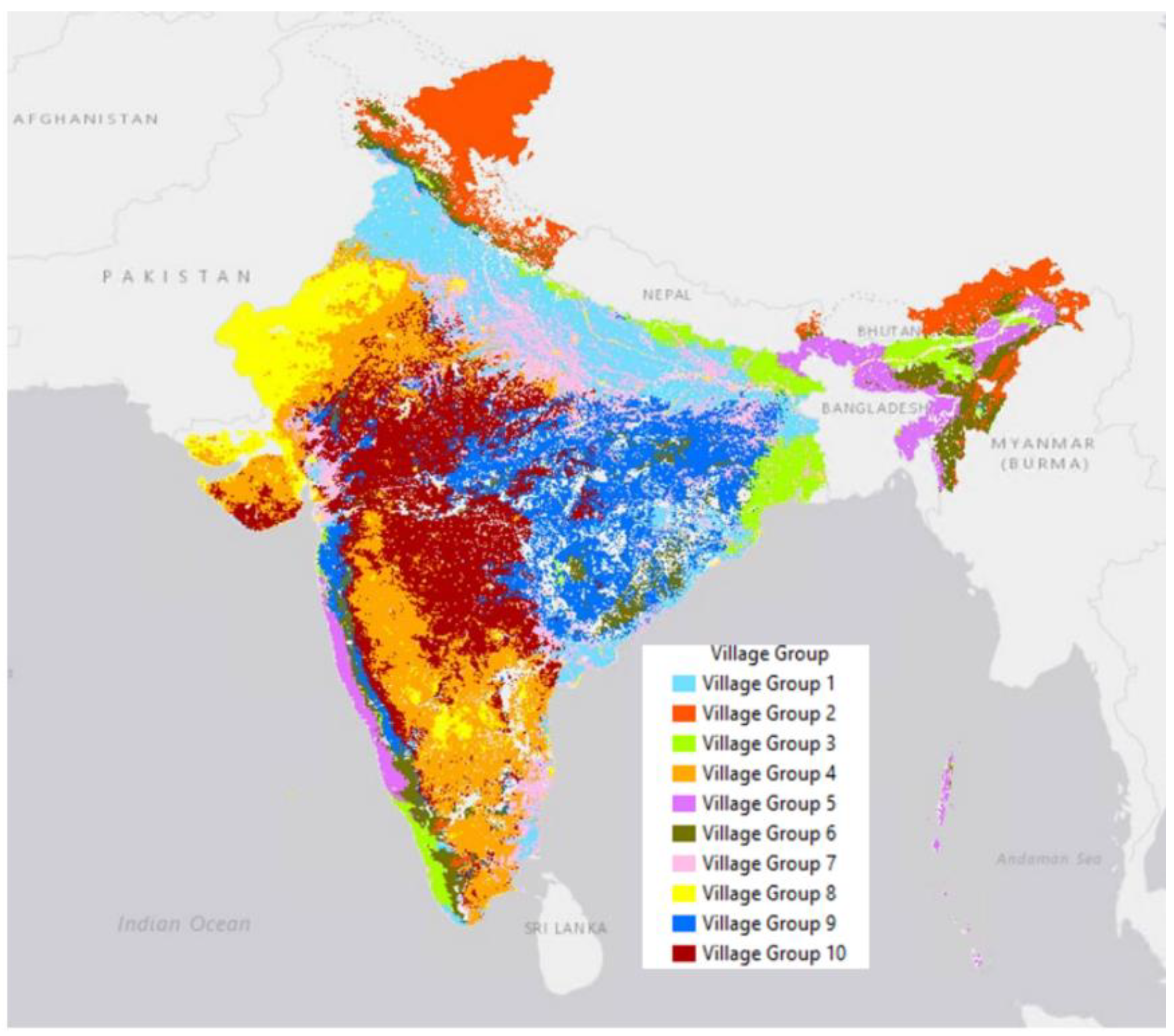
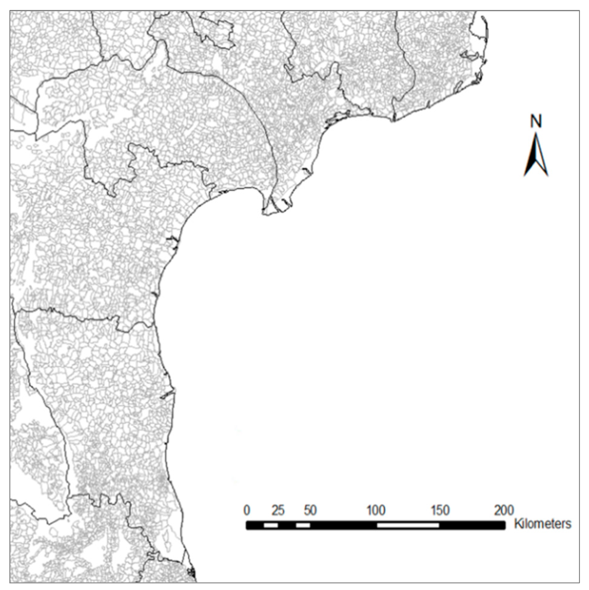
Figure 5 shows the spatial patterns of Indian villages based on the combined environmental conditions regarding vegetation, climate, and terrain. The whole country has 605,652 villages, with the majority of villages in group 9 and group 10 located in the central regions, group 1 located in the northern region, group 4 located in the southern region, group 3 located in the eastern and southern regions, and group 7 located in the northern and southern regions. Table 1, Table 2, Table 3, Table 4, Table 5, Table 6, Table 7, Table 8, Table 9 and Table 10 show the statistical characteristics of each village group for the five environmental variables, respectively. The village groups account for 20.74% (Group 1), 4.04% (Group 2), 9.85% (Group 3), 9.49% (Group 4), 4.64% (Group 5), 6.09% (Group 6), 13.70% (Group 7), 2.29% (Group 8), 15.35% (Group 9), and 13.81% (Group 10) of the total number of villages in the country.
Group 1 villages are characterized by NDVI value ranges between 0.52 and 0.97 with an average of 0.80, LST value ranges between 0.00 °C and 35.26 °C with an average of 29.81 °C, annual total RF value ranges between 0.00 mm and 1566.25 mm with an average of 1151.55 mm, elevation value ranges between 0.00 m and 932.34 m with an average of 127.92 m, and slope value ranges between 0.17 degrees and 10.64 degrees with an average of 0.72 degrees (Table 1).
Group 2 villages are characterized by NDVI value ranges between 0.02 and 0.97 with an average of 0.83, LST value ranges between −6.09 °C and 30.84 °C with an average of 21.35 °C, annual total RF value ranges between 98.04 mm and 4118.89 mm with an average of 1299.15 mm, elevation value ranges between 533.41 m and 5707.84 m with an average of 1729.28 m, and slope value ranges between 2.11 degrees and 43.03 degrees with an average of 22.84 degrees (Table 2).
Group 3 villages are characterized by NDVI value ranges between 0.29 and 0.99 with an average of 0.81, LST value ranges between 0.00 °C and 36.66 °C with an average of 28.44 °C, annual total RF value ranges between 797.23 mm and 2608.98 mm with an average of 1832.66 mm, elevation value ranges between 0.00 m and 848.79 m with an average of 67.45 m, and slope value ranges between 0.00 degrees and 11.48 degrees with an average of 0.98 degrees (Table 3).
Group 4 villages are characterized by NDVI value ranges between 0.42 and 0.75 with an average of 0.61, LST value ranges between 20.47 °C and 44.36 °C with an average of 36.66 °C, annual total RF value ranges between 0.00 mm and 1823.07 mm with an average of 650.12 mm, elevation value ranges between 0.76 m and 1778.38 m with an average of 433.27 m, and slope value ranges between 0.11 degrees and 20.61 degrees with an average of 1.45 degrees (Table 4).
Group 5 villages are characterized by NDVI value ranges between 0.29 and 0.99 with an average of 0.82, LST value ranges between 0.00 °C and 37.25 °C with an average of 27.07 °C, annual total RF value ranges between 2062.85 mm and 4975.36 mm with an average of 2988.49 mm, elevation value ranges between 0.01 m and 1735.62 m with an average of 141.75 m, and slope value ranges between 0.00 degrees and 30.77 degrees with an average of 3.31 degrees (Table 5).
Group 6 villages are characterized by NDVI value ranges between 0.52 and 0.99 with an average of 0.85, LST value ranges between 18.06 °C and 37.25 °C with an average of 26.41 °C, annual total RF value ranges between 393.01 mm and 4267.21 mm with an average of 1613.39 mm, elevation value ranges between 69.71 m and 2003.09 m with an average of 836.06 m, and slope value ranges between 0.00 degrees and 30.65 degrees with an average of 12.31 degrees (Table 6).
Group 7 villages are characterized by NDVI value ranges between 0.29 and 0.76 with an average of 0.68, LST value ranges between 0.00 °C and 38.16 °C with an average of 31.54 °C, annual total RF value ranges between 0.00 mm and 2911.00 mm with an average of 1191.62 mm, elevation value ranges between 0.00 m and 1585.78 m with an average of 148.82 m, and slope value ranges between 0.00 degrees and 16.29 degrees with an average of 0.99 degrees (Table 7).
Group 8 villages are characterized by NDVI value ranges between −0.10 and 0.51 with an average of 0.37, LST value ranges between 0.00 °C and 45.15 °C with an average of 36.63 °C, annual total RF value ranges between 0.00 mm and 3423.64 mm with an average of 654.81 mm, elevation value ranges between 0.00 m and 1831.09 m with an average of 202.76 m, and slope value ranges between 0.00 degrees and 29.11 degrees with an average of 1.23 degrees (Table 8).
Group 9 villages are characterized by NDVI value ranges between 0.60 and 0.98 with an average of 0.79, LST value ranges between 24.10 °C and 39.49 °C with an average of 32.33 °C, annual total RF value ranges between 550.91 mm and 2570.69 mm with an average of 1504.18 mm, elevation value ranges between 3.80 m and 1157.98 m with an average of 352.06 m, and slope value ranges between 0.27 degrees and 15.95 degrees with an average of 2.63 degrees (Table 9).
Group 10 villages are characterized by NDVI value ranges between 0.58 and 0.92 with an average of 0.75, LST value ranges between 30.22 °C and 43.07 °C with an average of 36.71 °C, annual total RF value ranges between 185.72 mm and 2233.93 mm with an average of 1119.78 mm, elevation value ranges between 3.66 m and 1135.93 m with an average of 402.32 m, and slope value ranges between 0.28 degrees and 16.42 degrees with an average of 1.69 degrees (Table 10).
The minimum values of zero for some variables in the tables are caused by a few villages without valid satellite data, but the impacts can be neglectable based on our analysis of the histograms. Figure 6, Figure 7, Figure 8, Figure 9 and 
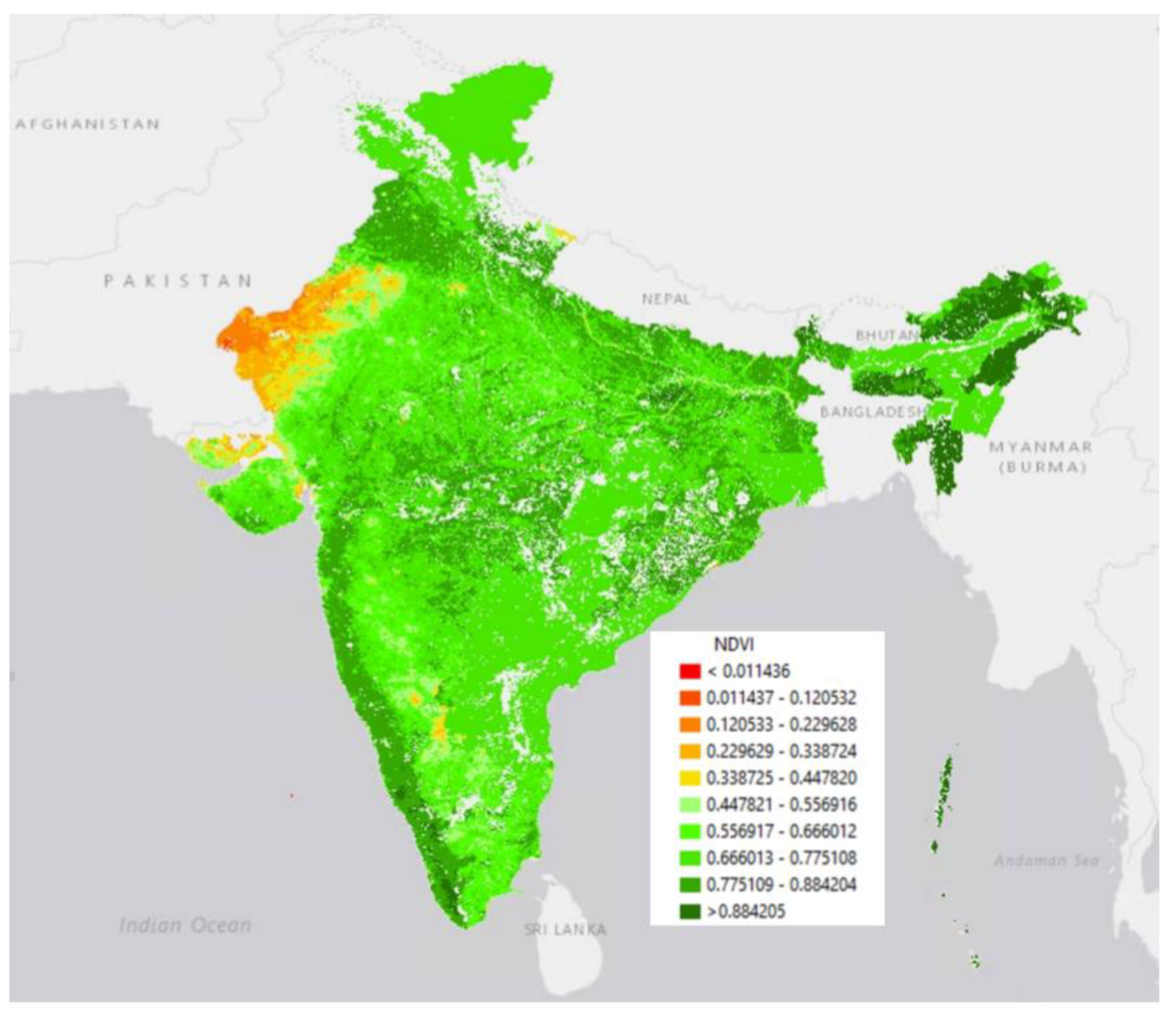
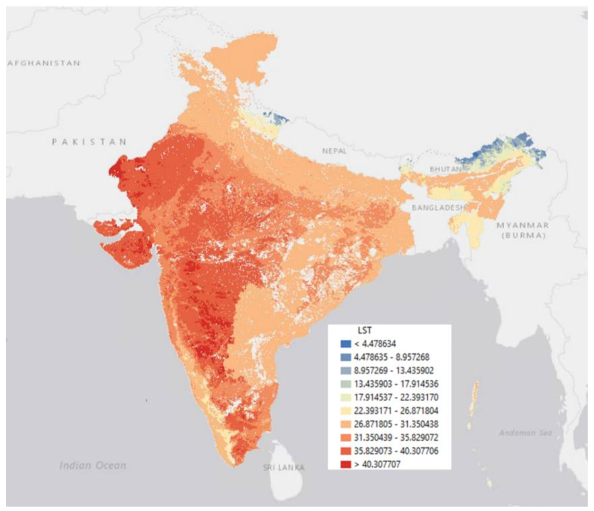
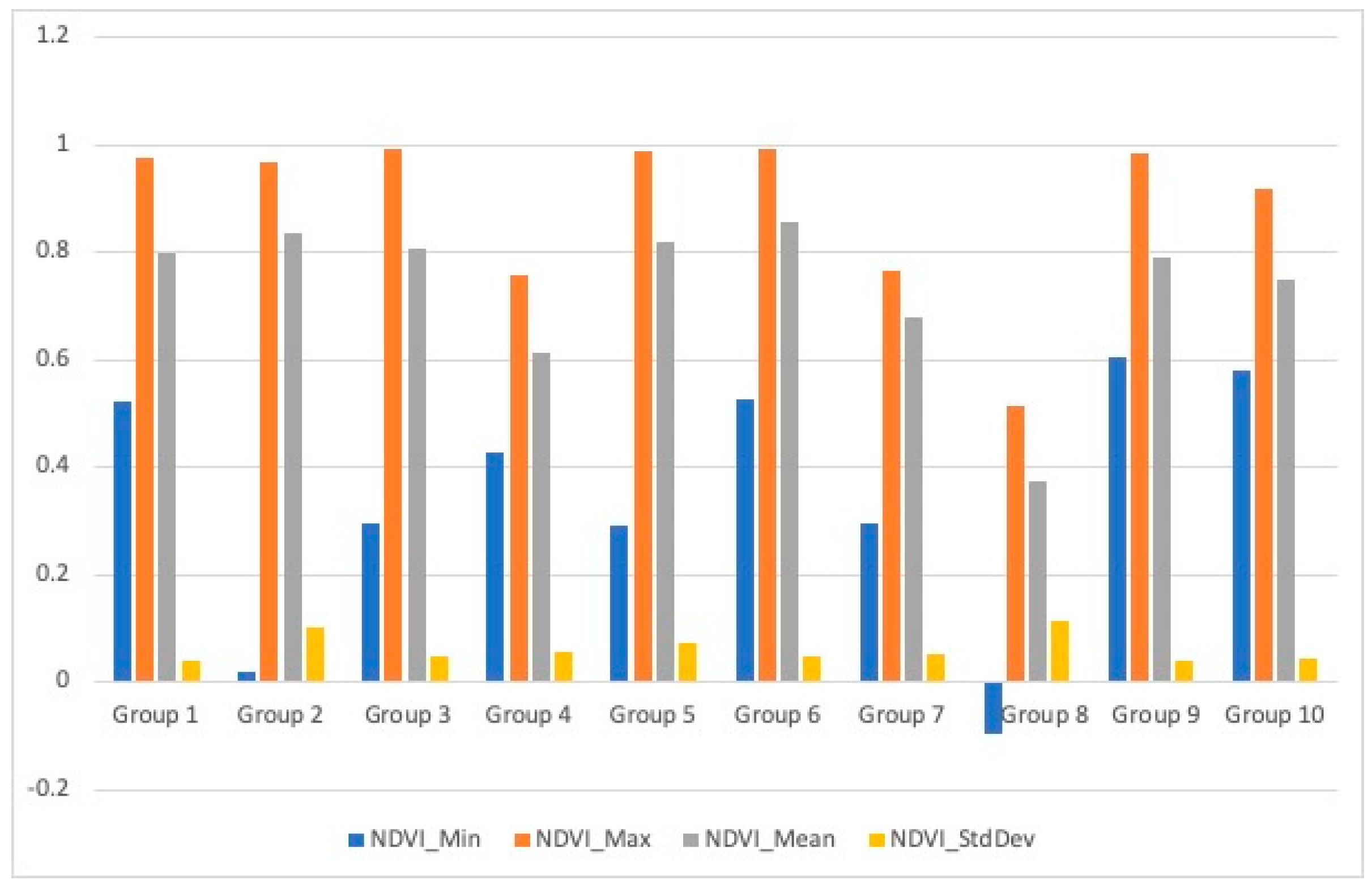
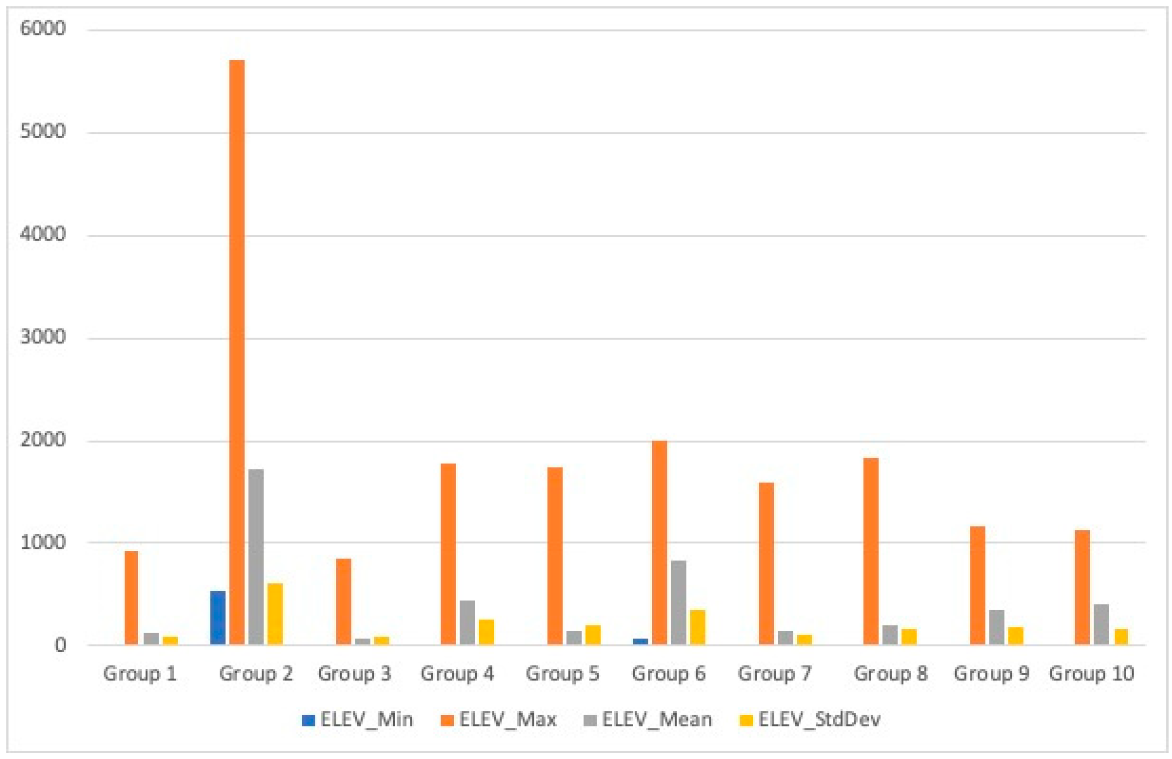
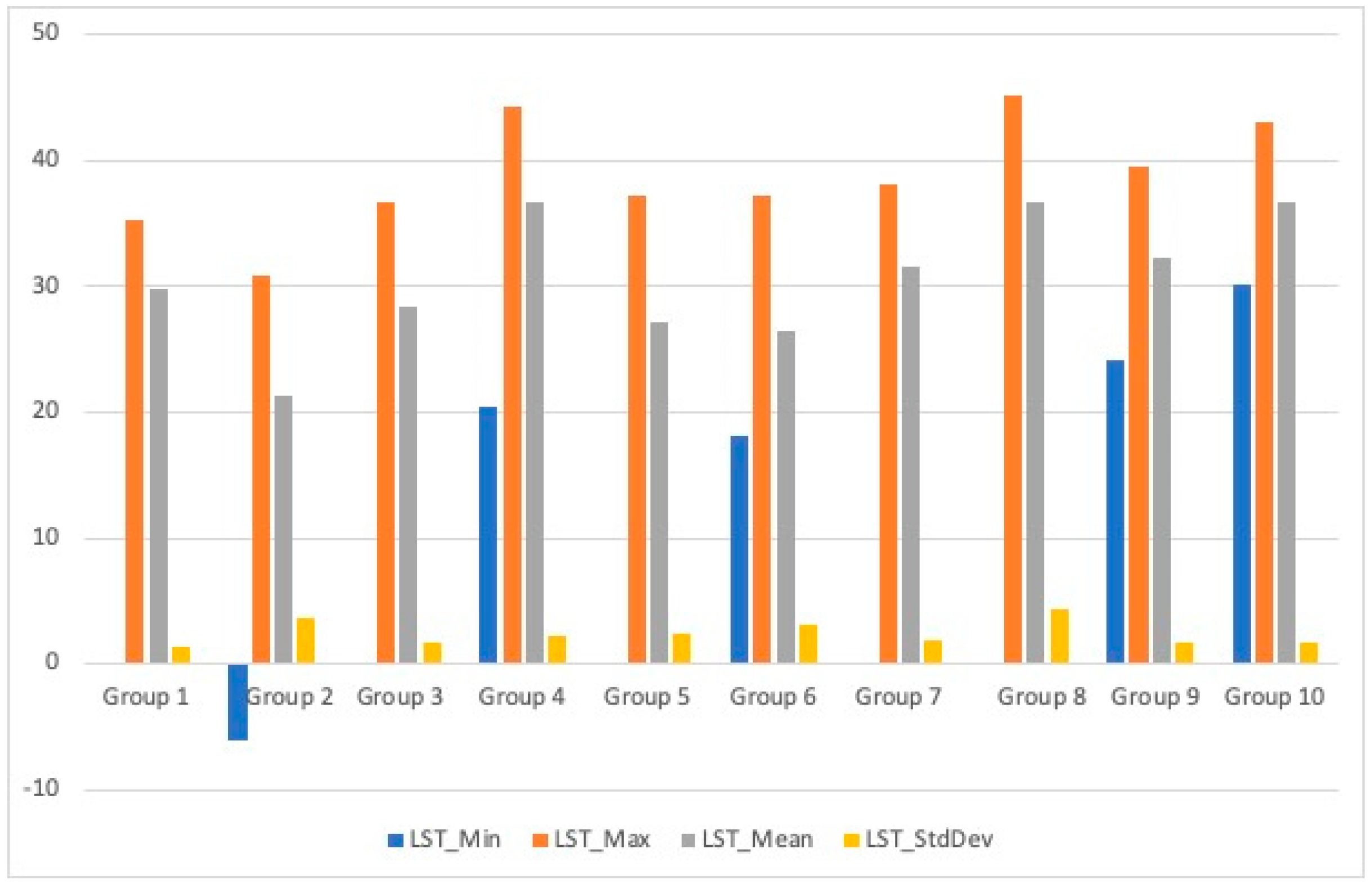
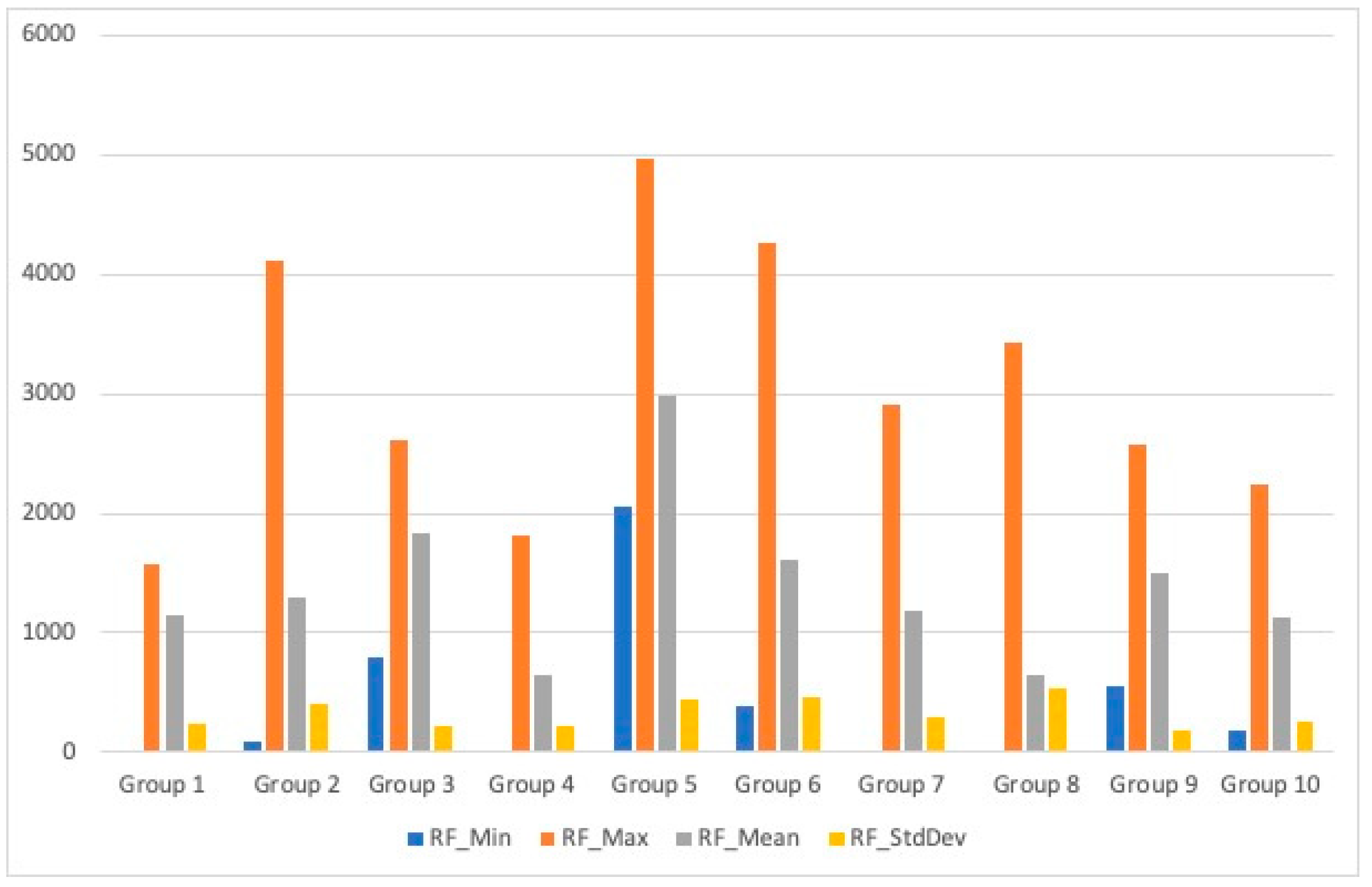
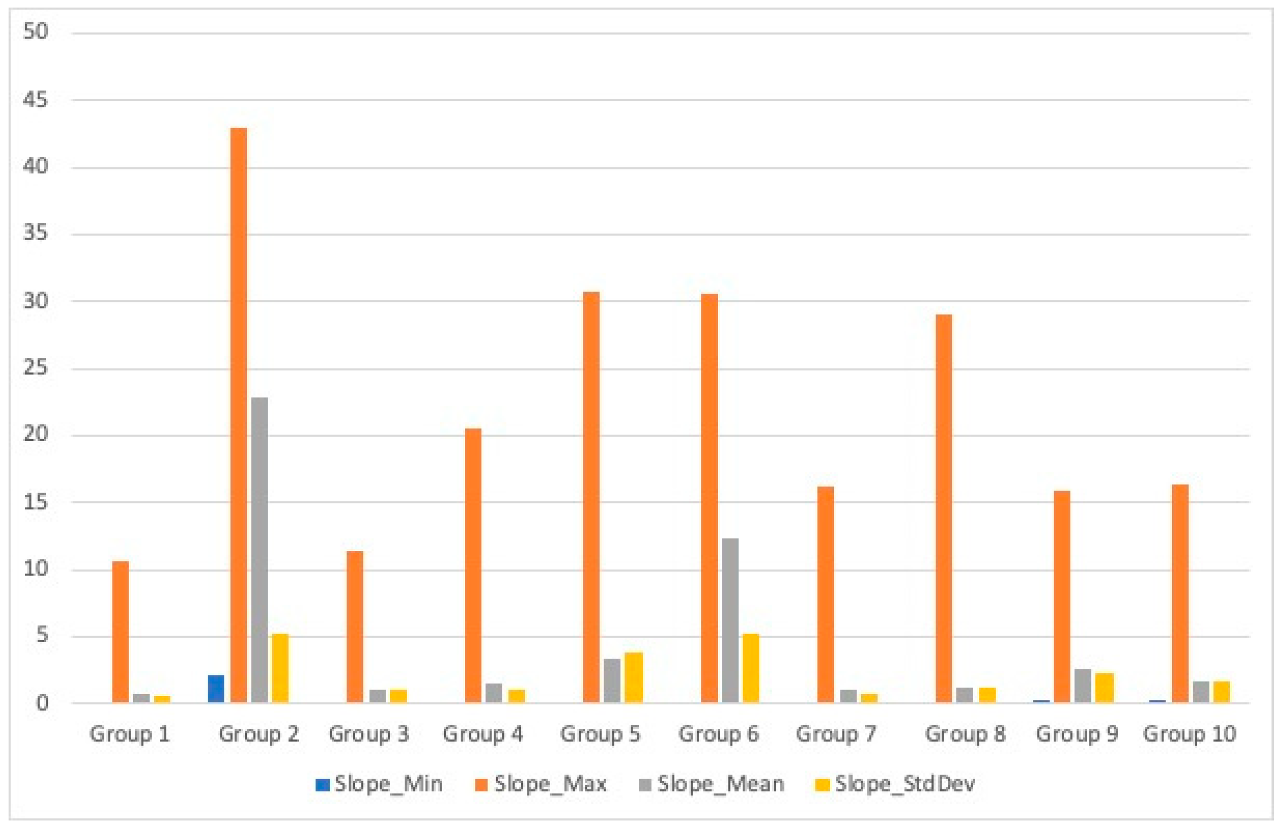
Figure 10 show the comparisons of environmental variables for all 10 village groups. Villages in groups 1, 2, 3, 5, 6, 9, and 10 all have high vegetation coverage, villages in groups 4 and 7 have moderate vegetation coverage, and villages in group 8 have lower vegetation coverage, with small within-group variations. All villages except those in group 2 have a higher land surface temperature, and all villages except those in groups 4 and 8 receive higher rainfalls. Villages in groups 2, 4, 5, 6, 7, and 8 are located in higher altitudes areas, with villages in groups 2, 5, 6, and 8 having steeper terrain.

3.2. Relationship between Environmental Variables and Child Malnutrition Indicators

Statistics for stunting, underweight, and wasting are calculated for each of the village groups identified through spatial analysis above, and the average values for all three child malnutrition indicators and the corresponding five environmental variables are shown in Table 11.
Based on statistical data from Table 11, a correlation analysis was performed between stunting, underweight, and wasting and the five environmental variables, and the correlation coefficients are shown in Table 12. It reveals that child stunting, underweight, and wasting all are negatively correlated to the vegetation index (NDVI), rainfall (RF), elevation, and slope, while positively correlated to land surface temperature (LST). In addition, while child stunting, underweight, and wasting are all correlated to all five environmental variables, stunting and underweight are more correlated to slope, elevation, and land surface temperature than rainfall and the vegetation index, and wasting is more correlated to land surface temperature and slope than the vegetation index, rainfall, and elevation. Further, the vegetation index, land surface temperature, and rainfall all are more correlated to wasting than underweight and stunting, while elevation and slope are more correlated to stunting and underweight than wasting.

4. Discussion

We have demonstrated a process to effectively derive environmental variables at the village level from satellite big datasets on a cloud platform for SDG research and applications. Spatial analysis of the environmental variables regarding vegetation, climate, and terrain have shown spatial grouping patterns across the entire study area, with each village group having different statistics. Correlation analysis between environmental variables and child stunting, underweight, and wasting show a meaningful relationship between these indicators and the vegetation index, land surface temperature, rainfall, elevation, and slope. The negative correlations between all three indicators and the vegetation index, rainfall, elevation, and slope, and the positive correlation between these indicators and land surface temperature are all reasonable because low vegetation index values indicate reduced vegetation productivity or stressed vegetation growth, low rainfall relates to reduced vegetation productivity, areas with low elevation and slope are more likely impacted by natural disasters such as floods, and all of these lead to less nutrition available to children and therefore higher child stunting, underweight, and wasting values. The positive correlation between stunting, underweight, and wasting with land surface temperature may be due to high temperatures potentially causing drought, thus leading to less available nutrition, and elevating these indicator values.
Identifying spatial variation patterns of environmental variables at the village level and their correlation with child malnutrition indicators can be an invaluable tool to facilitate a clearer understanding of the causes of child malnutrition and to improve area-specific SDG 3 implementation planning. For example, constrained by the environmental conditions of villages in a specific region, governments might choose to focus on other socioeconomic variables, such as improving nutrition policy for these villages. This analysis can also provide meaningful support in assessing and monitoring public health–related SDG implementation progress by spatially predicting such SDG indicators for the villages without indicator values estimated from surveys through incorporating environmental variables into socioeconomic independent variables.
There are many other environmental factors affecting public health–related SDGs that are not included in this study, such as air quality, water quality, and soil characteristics, which should be considered in further studies. In addition, the spatial grouping of villages should be updated when environmental variables change, especially for vegetation and climate related variables, as they are prone to change over time. This paper is just the first study to showcase the spatial variations of typical environmental variables related to public health SDGs at the village level and the relationships between these variables and the specific SDG 3 relevant indicators. The methodology has the potential to be applied to other similar regions, especially low-to-middle income countries where a high number of children are severely affected by malnutrition, as well as to other environmentally related SDGs, such as Goal 1 (No Poverty) and Goal 2 (Zero Hunger).

Author Contributions

R.K., S.V.S. and X.L.: conceptualization and research design; X.L. and W.Z.: data processing and analysis; X.L., R.K., W.Z., W.W.G. and S.V.S.: results assessment and suggestions; W.W.G., S.V.S. and R.K.: project administration and funding acquisition; X.L.: original draft preparation; R.K., W.Z., W.W.G., S.V.S. and X.L.: review and editing. All authors have read and agreed to the published version of the manuscript.

Funding

This research is funded by BMGF INV-002992 and NSF Award Number 1841403.

Institutional Review Board Statement

Ethical review and approval were waived for this study due to the use of publicly accessible secondary data with no identifiers. This research does not meet the regulatory definition of human subject research.

Informed Consent Statement

Not applicable.

Data Availability Statement

DHS data are available at https://dhsprogram.com (requiring a simple application). Satellite environmental data are available when requested.

Conflicts of Interest

The authors declare no conflict of interest.

References

  1. United Nations. Transforming Our world: The 2030 Agenda for Sustainable Development. 2015. Available online: https://sustainabledevelopment.un.org/post2015/transformingourworld/publication (accessed on 10 May 2022).
  2. United Nations. Report of the Inter-Agency and Expert Group on Sustainable Development Goal Indicators (Revised). 2016. Available online: https://www.healthdatacollaborative.org/fileadmin/uploads/hdc/Documents/Final_list_of_proposed_Sustainable_Development_Goal_indicators.pdf (accessed on 15 July 2022).
  3. Bhanja, R.; Roychowdhury, K. Assessing the progress of India towards sustainable development goals by 2030. J. Glob. Resour. 2020, 6, 81–91. [Google Scholar] [CrossRef]
  4. Rekha, B. Geospatial Data: Key to Achieve SDGs. Geospatial World. 2016. Available online: https://www.geospatialworld.net/article/geospatial-data-sustainable-development-goals/ (accessed on 10 May 2022).
  5. MacFeely, S. The big (data) bang: Opportunities and challenges for compiling SDG indicators. Glob. Policy 2019, 10, 121–133. [Google Scholar] [CrossRef]
  6. Kim, R.; Bijral, A.S.; Xu, Y.; Zhang, X.; Blossom, J.C.; Swaminathan, A.; King, G.; Kumar, A.; Sarwal, R.; Ferres, J.M.L.; et al. Precision mapping child undernutrition for nearly 600,000 inhabited census villages in India. Proc. Natl. Acad. Sci. USA 2021, 118, e2025865118. [Google Scholar] [CrossRef] [PubMed]
  7. Moallemi, E.; Malekpour, A.S.; Hadjikakou, M.; Raven, R.; Szetey, K.; Ningrum, D.; Dhiaulhaq, A.; Bryan, B.A. Achieving the sustainable development goals requires transdisciplinary innovation at the local scale. One Earth 2020, 3, 300–313. [Google Scholar] [CrossRef]
  8. IHME. The Global Burden of Disease: Generating Evidence, Guiding Policy; IHME: Seattle, WA, USA, 2013. [Google Scholar]
  9. Annan, K. Data can help to end malnutrition across Africa. Nature 2018, 555, 7. [Google Scholar] [CrossRef] [PubMed]
  10. Dowell, S.F.; Blazes, D.; Desmond-Hellmann, S. Four steps to precision public health. Nature 2016, 540, 189–191. [Google Scholar] [CrossRef]
  11. Kim, R.; Mohanty, S.K.; Subramanian, S. Multilevel geographies of poverty in India. World Dev. 2016, 87, 349–359. [Google Scholar] [CrossRef]
  12. Kim, R.; Kawachi, I.; Coull, B.A.; Subramanian, S.V. Contribution of socioeconomic factors to the variation in body-mass index in 58 low-income and middle-income countries: An econometric analysis of multilevel data. Lancet Glob. Health 2018, 6, e777–e786. [Google Scholar] [CrossRef]
  13. Reich, B.J.; Haran, M. Precision maps for public health. Nature 2018, 555, 32–33. [Google Scholar] [CrossRef] [PubMed]
  14. Horton, R. Offline: In defence of precision public health. Lancet 2018, 392, 1504. [Google Scholar] [CrossRef]
  15. Xie, Y.; Sha, Z.; Yu, M. Remote sensing imagery in vegetation mapping: A review. J. Plant Ecol. 2008, 1, 9–23. [Google Scholar] [CrossRef]
  16. Lechner, A.M.; Foody, G.M.; Boyd, D.S. Applications in remote sensing to forest ecology and management. One Earth 2020, 2, 405–412. [Google Scholar] [CrossRef]
  17. Mzid, N.; Cantore, V.; Mastro, G.D.; Albrizio, R.; Sellami, M.H.; Todorovic, M. The application of ground-based and satellite remote sensing for estimation of bio-physiological parameters of wheat grown under different water regimes. Water 2020, 12, 2095. [Google Scholar] [CrossRef]
  18. Ali, I.; Cawkwell, F.; Dwyer, E.; Barrett, B.; Green, S. Satellite remote sensing of grasslands: From observation to management. J. Plant Ecol. 2016, 9, 649–671. [Google Scholar] [CrossRef]
  19. Avtar, R.; Komolafe, A.A.; Kouser, A.; Singh, D.; Yunus, A.P.; Dou, J.; Kumar, P.; Gupta, R.D.; Johnson, B.A.; Minh, H.V.T.; et al. Assessing sustainable development prospects through remote sensing: A review. Remote Sens. Appl. Soc. Environ. 2020, 20, 100402. [Google Scholar] [CrossRef] [PubMed]
  20. Ferreira, B.; Iten, M.; Silva, R.G. Monitoring sustainable development by means of earth observation data and machine learning: A review. Environ. Sci. Eur. 2020, 32, 120. [Google Scholar] [CrossRef]
  21. Solanky, V.; Singh, S.; Katiyar, S.K. Land surface temperature estimation using remote sensing data. In Hydrologic Modeling. Water Science and Technology Library; Singh, V., Yadav, S., Yadava, R., Eds.; Springer: Singapore, 2018; Volume 81. [Google Scholar] [CrossRef]
  22. Sadeghi, M.; Shearer, E.J.; Mosaffa, H.; Gorooh, V.A.; Naeini, M.R.; Hayatbini, N.; Katiraie-Boroujerdy, P.; Analui, B.; Mguyen, P.; Sorooshian, S. Application of remote sensing precipitation data and the CONNECT algorithm to investigate spatiotemporal variations of heavy precipitation: Case study of major floods across Iran (Spring 2019). J. Hydrol. 2021, 600, 126569. [Google Scholar] [CrossRef]
  23. Barrett, E.C. Satellite remote sensing of precipitation: Progress and problems. Remote Sens. Hydrol. 2001, 2000, 3–10. [Google Scholar]
  24. Didan, K.; Munoz, A.B.; Solano, R.; Huete, A. MODIS Vegetation Index User’s Guide (MOD13 Series). 2015. Available online: https://vip.arizona.edu/documents/MODIS/MODIS_VI_UsersGuide_June_2015_C6.pdf (accessed on 10 May 2022).
  25. Wan, Z. Collection-6 MODIS Land Surface Temperature Products Users’ Guide. 2019. Available online: https://lpdaac.usgs.gov/documents/715/MOD11_User_Guide_V61.pdf (accessed on 10 May 2022).
  26. UCSB. CHIRPS: Rainfall Estimates from Rain Gauge and Satellite Observations. 2022. Available online: https://www.chc.ucsb.edu/data/chirps (accessed on 11 May 2022).
  27. NASA. U.S. Releases Enhanced Shuttle Land Elevation Data. 2022. Available online: https://www2.jpl.nasa.gov/srtm/ (accessed on 10 May 2022).
  28. Shekhar, S.; Xiong, H.; Zhou, X. Statistical descriptions of spatial patterns. In Encyclopedia of GIS; Shekhar, S., Xiong, H., Zhou, X., Eds.; Springer: Cham, Switzerland, 2017; pp. 81–92. [Google Scholar] [CrossRef]
  29. Alzaghoul, E.; Al-Zoubi, M.B.; Obiedat, R.; Alzaghoul, F. Applying machine learning to DEM raster images. Technologies 2021, 9, 87. [Google Scholar] [CrossRef]
  30. Meredith, T.N.; Emery, B.F.; Wiltshire, S.; Brown, M.E.; Fisher, B.; Ricketts, T.H. Climate impacts associated with reduced diet diversity in children across nineteen countries. Environ. Res. Lett. 2021, 16, 015010. [Google Scholar]
Figure 1. Village boundary data illustrated relative to district boundaries. All administrative boundary data layers are provided by the Geographic Insights Lab of the Center for Population and Development Studies at Harvard University.
Sustainability 14 10450 g001
Figure 2. Village-level 2016 NDVI dataset derived from satellite data.
Sustainability 14 10450 g002
Figure 3. Village-level 2016 LST dataset derived from satellite data.
Sustainability 14 10450 g003
Figure 4. Village-level samples of child malnutrition indicators calculated from DHS data.
Sustainability 14 10450 g004
Figure 5. Village-level environmental spatial variation patterns combining vegetation index, land surface temperature, rainfall, elevation, and slope.
Sustainability 14 10450 g005
Figure 6. Statistical characteristics of normalized difference vegetation index (NDVI) for different village groups with higher values indicating higher coverage of vegetation.
Sustainability 14 10450 g006
Figure 7. Statistical characteristics of land surface temperature (LST in °C) for different village groups with higher values indicating warmer areas.
Sustainability 14 10450 g007
Figure 8. Statistical characteristics of rainfall (RF in mm) with higher values indicating more rainfall.
Sustainability 14 10450 g008
Figure 9. Statistical characteristics of elevation (ELEV in m) with higher values indicating higher altitudes.
Sustainability 14 10450 g009
Figure 10. Statistical characteristics of slope (in degrees) with higher values indicating steeper terrain areas.
Sustainability 14 10450 g010
Table 1. Statistical characteristics of environmental variables in Village Group 1.
Total Number of Villages: 125,606 (20.74% of the Total Villages)
MinMaxMeanStd Dev
NDVI0.5230560.9761330.7993110.041414
LST (°C)0.00000035.25999529.8067651.387735
RF (mm)0.0000001566.2471901151.551969236.219450
Elevation (m)0.000000932.337288127.92416081.830367
Slope (degree)0.17400310.6391140.7251220.547874
Table 2. Statistical characteristics of environmental variables in Village Group 2.
Total Number of Villages: 24,487 (4.04% of the Total Villages)
MinMaxMeanStd Dev
NDVI0.0187230.9691230.8347520.101169
LST (°C)−6.08743330.83686721.3497693.700455
RF (mm)98.042874118.8882761299.147316407.588644
Elevation (m)533.4080725707.8350421729.277104613.499489
Slope (degree)2.11019243.02617522.8441505.158610
Table 3. Statistical characteristics of environmental variables in Village Group 3.
Total Number of Villages: 59,640 (9.85% of the Total Villages)
MinMaxMeanStd Dev
NDVI0.2939330.9918000.8067060.047967
LST (°C)0.00000036.66342828.4400011.650479
RF (mm)797.2336362608.9846081832.655345226.825014
Elevation (m)0.000000848.79268367.45184694.647125
Slope (degree)0.00000011.4797580.9847671.052747
Table 4. Statistical characteristics of environmental variables in Village Group 4.
Total Number of Villages: 57,460 (9.49% of the Total Villages)
MinMaxMeanStd Dev
NDVI0.4263820.7589540.6127780.056437
LST (°C)20.47404844.36300436.6594482.292870
RF (mm)0.0000001823.074413650.125899216.674174
Elevation (m)0.7632541778.379032433.272696265.338206
Slope (degree)0.11252820.6062111.4547051.052747
Table 5. Statistical characteristics of environmental variables in Village Group 5.
Total Number of Villages: 28,070 (4.64% of the Total Villages)
MinMaxMeanStd Dev
NDVI0.2902130.9891000.8197430.074932
LST (°C)0.00000037.24654927.0743712.388734
RF (mm)2062.8481034975.365932988.492576437.467212
Elevation (m)0.0130431735.623457141.747258206.672506
Slope (degree)0.00444230.7694513.3094153.883592
Table 6. Statistical characteristics of environmental variables in Village Group 6.
Total Number of Villages: 36,889 (6.09% of the Total Villages)
MinMaxMeanStd Dev
NDVI0.5255110.9938000.8546170.047670
LST (°C)18.06476837.24808126.4106553.099043
RF (mm)393.0131954267.2109101613.386441469.675848
Elevation (m)69.7142862003.092593836.058964347.582120
Slope (degree)0.00000030.64779012.3075225.271495
Table 7. Statistical characteristics of environmental variables in Village Group 7.
Total Number of Villages: 82,952 (13.70% of the Total Villages)
MinMaxMeanStd Dev
NDVI0.2949970.7656020.6779160.051785
LST (°C)0.00000038.15787231.5458641.850205
RF (mm)0.0000002911.005781191.622396287.46317
Elevation (m)0.0000001585.782051148.820066104.197068
Slope (degree)0.00000016.2894290.9951690.794141
Table 8. Statistical characteristics of environmental variables in Village Group 8.
Total Number of Villages: 13,893 (2.29% of the Total Villages)
MinMaxMeanStd Dev
NDVI−0.0976600.5123930.3721680.113446
LST (°C)0.00000045.14661936.6273674.439418
RF (mm)0.0000003423.642334654.810119538.491456
Elevation (m)0.0000001831.093333202.763915169.987659
Slope (degree)0.00000029.1124591.2327291.191413
Table 9. Statistical characteristics of environmental variables in Village Group 9.
Total Number of Villages: 92,989 (15.35% of the Total Villages)
MinMaxMeanStd Dev
NDVI0.6030460.9824000.7896820.042110
LST (°C)24.10403339.49122832.3328641.645638
RF (mm)550.9174372570.6892911504.179448181.292221
Elevation (m)3.8055561157.978261352.063712182.009354
Slope (degree)0.27296315.9505972.6341492.314364
Table 10. Statistical characteristics of environmental variables in Village Group 10.
Total Number of Villages: 83,666 (13.81% of the Total Villages)
MinMaxMeanStd Dev
NDVI0.5812710.9201400.7486880.043622
LST (°C)30.21647243.07545436.7142661.707098
RF (mm)185.7160552233.7497071119.779193263.945674
Elevation (m)3.6601941135.929412402.325718169.629362
Slope (degree)0.28434116.4199461.6924781.708024
Table 11. Average child malnutrition indicators and corresponding environmental variables for each of the village groups.
Village GroupStuntingUnderweightWastingNDVILST (°C)RF (mm)Elevation (m)Slope (Degree)
10.3988810.3534510.1822960.79931129.8067651151.552127.92420.725122
20.2930090.1879490.1507760.83475221.3497691299.1471729.27722.84415
30.3529910.3025250.1648170.80670628.4400011832.65567.451850.984767
40.338720.3230850.2149570.61277836.659448650.1259433.27271.454705
50.3155960.2577650.1667010.81974327.0743712988.493141.74733.309415
60.3047960.2009430.1331260.85461726.4106551613.386836.05912.307522
70.4119250.3783340.2018860.67791631.5458641191.622148.82010.995169
80.3653570.3511290.2235730.37216836.627367654.8101202.76391.232729
90.3899330.4127330.2577480.78968232.3328641504.179352.06372.634149
100.3991180.4100260.2522290.74868836.7142661119.779402.32571.692478
Table 12. Correlation between child malnutrition indicators and environmental variables.
StuntingUnderweightWastingNDVILST (°C)RF (mm)Elevation (m)Slope (Degree)
Stunting1
Underweight0.9344440631
Wasting0.7061421800.8958421141
NDVI−0.269744102−0.382935060−0.468491
LST (°C)0.6270892790.7926915790.822567−0.70084511
RF (mm)−0.365031717−0.370347674−0.431930.608719−0.5511281
Elevation (m)−0.639507126−0.654425393−0.387030.3034617−0.586226−0.117381
Slope (degree)−0.725057292−0.782828143−0.568440.3987414−0.7529910.077380.9660591
Publisher’s Note: MDPI stays neutral with regard to jurisdictional claims in published maps and institutional affiliations.

