Article

The Multi-Depot Traveling Purchaser Problem with Shared Resources

by
Zahra Sadat Hasanpour Jesri
1,
Kourosh Eshghi
1,
Majid Rafiee
1,* and
Tom Van Woensel
2
1
Department of Industrial Engineering, Sharif University of Technology, Tehran 11155-9465, Iran
2
School of Industrial Engineering, Eindhoven University of Technology, 5612 AZ Eindhoven, The Netherlands
*
Author to whom correspondence should be addressed.
Sustainability 2022, 14(16), 10190; https://doi.org/10.3390/su141610190
Submission received: 23 June 2022 / Revised: 8 August 2022 / Accepted: 9 August 2022 / Published: 17 August 2022

Abstract

:
Using shared resources has created better opportunities in the field of sustainable logistics and procurement. The Multi-Depot Traveling Purchaser Problem under Shared Resources (MDTPPSR) is a new variant of the Traveling Purchaser Problem (TPP) in sustainable inbound logistics. In this problem, each depot can purchase its products using the shared resources of other depots, and vehicles do not have to return to their starting depots. The routing of this problem is a Multi-Trip, Open Vehicle Routing Problem. A tailored integer programming model is formulated to minimize the total purchasers’ costs. Considering the complexity of the model, we have presented a decomposition-based algorithm that breaks down the problem into two phases. In the first phase, tactical decisions regarding supplier selection and the type of collaboration are made. In the second phase, the sequence of visiting is determined. To amend the decisions made in these phases, two heuristic algorithms based on the removing and insertion of operators are also proposed. The experimental results show that not only can purchasing under shared resources reduce the total cost by up to 29.11%, but it also decreases the number of dispatched vehicles in most instances.

1. Introduction

The stiff competition among different purchasing organizations means that companies have to look for more efficient ways to handle their procurement expenditure, constituting significant costs. Although the selection of suppliers and procurement resources is essential to cutting back a firm’s costs, there are no determining factors in procurement. Transportation cost is an indispensable component of the procurement cost and needs to be optimized [1]. The Traveling Purchaser Problem (TPP) is a well-known problem related to both purchasing and transportation costs [1]. It should be noted that TPP, a procurement logistics issue, has become a useful tool for corporate information systems when purchasing and collecting the required raw materials, spare parts, or their required items from potential suppliers. Meanwhile, TPP has applications in other domains such as school bus routing, the daily scheduling of surgeries, and so on [1]. That said, in this paper, we focus on its application in the field of procurements.
The common assumption about the traditional TPP in the literature is that there is only a central depot where vehicles depart from and arrive after visiting a subset of potential dispersed suppliers and deciding how much of each product to buy to meet the minimum demands, after considering traveling and purchasing costs [1]. Suppose that each purchaser performs its purchasing activities on its own. If the purchaser performs its purchasing activities independently, they may incur lots of losses due to underutilized vehicles, extra purchasing, and transportation costs. As mentioned earlier, transportation cost is a determining factor in procurement. Although there might be some inefficiencies in transportation, many companies are looking for more effective ways to reduce their costs based on cooperative pooled transport.
In the last decade, collaborative transportation has gained much more attention in both practical and academic domains. Many governments define incentive policies to promote collaboration among logistics enterprises [2]. For example, the city of Zurich has developed an online platform for further cooperation between transport units [3]. This project aimed to reduce the number of vehicles in urban last-mile delivery. NexTrust is another EU-funded project that focuses on the sustainable and environmental development of supply chains by reducing emission through using shared distribution resources in the logistics networks [4]. This study aimed to set up a platform for matching vacant capacities with delivery to improve delivery time and service level. In addition, by completing 40 pilot projects, CO2 emissions decreased by up to 20–70% [2].
Most of these collaborative transportation methods between companies have focused on the delivery process in outbound logistics. However, in the current study, we implement a cooperative structure for the purchasing and transporting of products between different purchasers. This structure seems fruitful, especially for those who work as a holding’s subsidiaries. More precisely, some companies such as Toyota Corporation create subsidiaries with their business model. Our proposed model can assist such holdings companies in reducing their overall procurement costs.
This paper proposes a Multi-Depot TPP under Shared Resources (MDTPPSR) model, according to which different purchasers can use the vehicle capacities of other purchasers to procure their products. In the Multi-Depot TPP (MDTPP), multiple independent depots (purchasers) purchase their specific required products from different potential suppliers. Suppose there is no joint structure between the depots. In that case, the MDTPP can be seen as many independent TPPs that can be solved individually by exact or heuristic algorithms available in the literature. In our model, different purchasers can collaborate on purchasing and loading the products of other purchasers. However, it bears noting that the products purchased by a specific vehicle must be delivered to its corresponding depot. A simple comparison of individual and collaborative purchasing is shown in Figure 1. Generally, in a network where different business units purchase their products individually, loading and delivering products can be far from efficient. Sometimes, huge losses are incurred due to their vehicles’ underutilization, and asset repositioning. However, via the demand-pooling of different purchasers in a joint collaborative network, they can benefit from their collaboration.
As shown in Figure 1a, neither business unit A nor unit B can effectively use their vehicle capacities. However, according to Figure 1b, aggregating the product demands, and collaborating, improves vehicle utilization. The number of required vehicles decreases, too. Moreover, in contrast to the classical TPP, where the same depot serves as both a particular vehicle’s point of departure and its point of arrival, in our model, the vehicle does not necessarily have to finish its journey at the same depot where it departed. Therefore, not only can the purchaser’s products be loaded by other purchasers’ vehicles, but depots’ resources are shared among different purchasers to avoid an unnecessary return to the initial depot. Note that the positions of the vehicles can be easily managed by the global positioning system and other information systems, and, accordingly, their parking status and available parking spaces at each depot can be controlled [5]. Given shared depots, transportation costs can decline thanks to the multiple choices in our route arrangement.
For example, consider a network with two purchasers and one supplier, as shown in Figure 2. If each purchaser purchases their products from the supplier (supplier X) individually, not only do they have to dispatch their vehicle to supplier X, but they also incur extra transportation costs (such as asset repositioning costs).
However, if two purchasers collaborate while increasing efficiency, this helps reduce transportation costs. Each vehicle is supposed to deliver each purchased product to its corresponding depot. In this case, we propose two routing approaches:
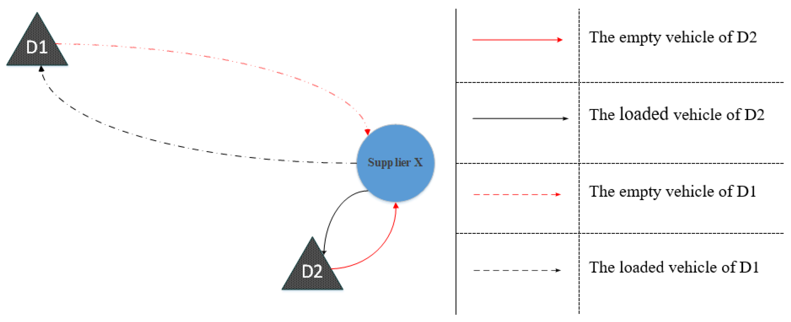
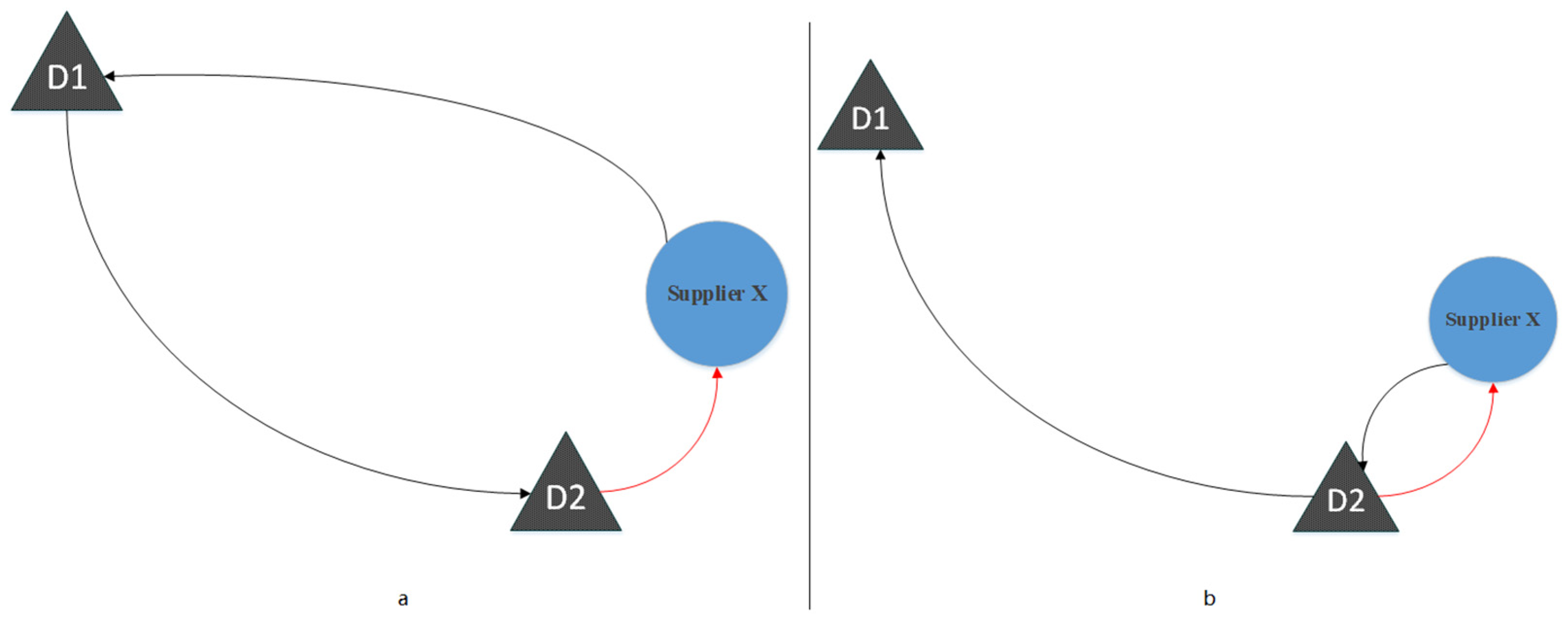
  • First approach—Each dispatched vehicle should return to its depot (its starting node) at the end of its route. Indeed, the route of each vehicle is a “closed route” or “circuit”. One drawback associated with this approach is that the corresponding depot of the vehicle is the last one that receives its purchased products (Figure 3a);
  • Second approach—Each vehicle can stay at the depot of the last purchaser whose products are delivered by this vehicle. Contrary to the first approach, the vehicle does not have to return to its starting depot (Figure 3b).
In the first approach (Figure 3a), with the collaboration of two purchasers, only one vehicle (the vehicle of depot D2) is dispatched to purchase the products of both depots from suppliers; transportation costs and deadheading costs have decreased compared to the individual case in Figure 2. As shown in Figure 3, the distance between supplier X and depot D2 is less than the distance to depot D1. In the second approach (Figure 3b), after the vehicle from depot D2 dispatches and visits supplier X, it first returns to its initial depot (D2) to deliver its purchased products. Then, to provide the products of depot D1, it is routed to depot D1 and stays there. Therefore, it does not have to get back to its starting depot.
The transportation cost (and the deadheading cost) of the second approach is lower than that of the first one. However, it bears noting that these assumptions are considered for a single periodic state, and, thus, by purchasing the products from supplier x, the purchase process is completed. Moreover, in the second approach, depot D2 receives its purchased products in a shorter time, while in the first approach, the dispatcher depot (D2) is the last one receiving its products. However, the second approach is more complex than the first one in terms of modeling and solving.
The two main differences between these approaches are outlined below:
-
Since each vehicle might continue its route after returning to its starting depot to deliver the products of others, each vehicle might make more than one trip (as is also the case with the Multi-trip Vehicle Routing Problem);
-
Suppose the vehicle returns to its initial depot and provides products to it, and then delivers the products to others. In that case, the routes are a combination of closed and open routes (similar to Figure 3b). We call the second proposed approach a “Multi-Trip, Open Vehicle Routing Problem”.
Our proposed framework is centralized, i.e., a central decision-maker tries to satisfy all purchasers’ demands at the minimum total cost. Therefore, the method of cost allocation is not the focus of our article. Centralized planning is defined as a stream of collaborative VRP in the literature, where a central authority makes collaborative decisions by having all the information. Based on [6], most of the contributions in centralized planning are intended to either present innovative models or innovative solution approaches, or to assess the potential gains of centralized collaborative planning versus a non-collaborative structure. In our paper, addressing the case of Multi-depot TPP, we are more concentrated on the first one. However, in our experimental analysis, the cost reduction is assessed, as well.
The contributions of this paper are threefold:
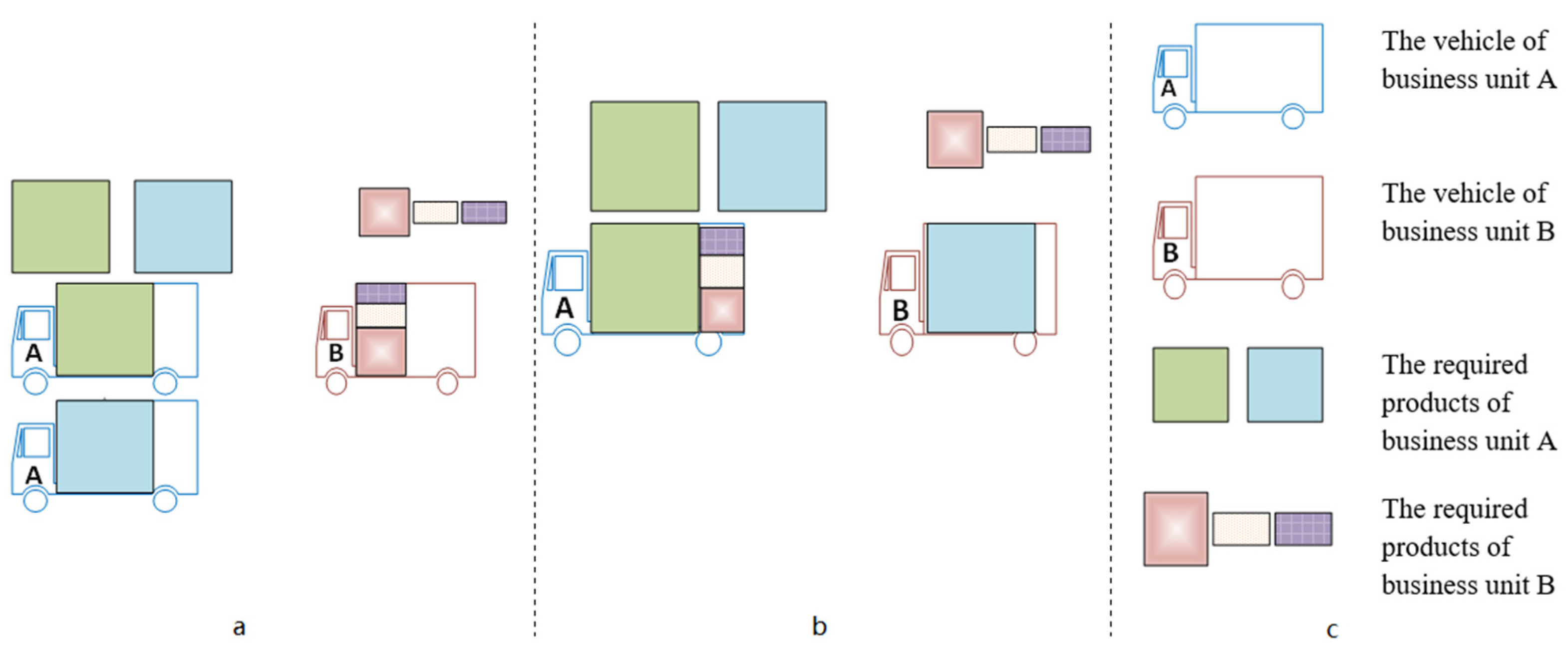
  • Modeling—In this paper, we design a collaborative structure between multiple purchasers for the sustainable development of procurement and the inbound logistics network. In this regard, we propose a mathematical model for MDTPPSR. In our model, we also define a collaborative rate ( α ) between depots, which ranges from 0 (a multi independent TPP) to 1 (full collaboration). In complete cooperation, the vehicle of a depot can load the products of other depots, even without loading one product from its depot. We perform some logical analysis to estimate the minimum number of required vehicles in partial collaboration ( 0 < α < 1 );
  • Introducing a new variant of the vehicle routing problem—As mentioned earlier, the collaboration structure between members is not just about using the shared vehicle capacities. Rather, it is also about the shared parking spaces of other depots. Regarding the second dimension of the collaboration framework (using the shared parking spaces), we introduce a new type of vehicle routing problem, “Multi-Trip, Open Vehicle Routing Problem”, which, to the best of the authors’ knowledge, has not been adequately addressed so far in the relevant literature. In this new type of routing problem, the vehicle of a particular depot is allowed to end at another depot’s parking space after delivering its products and those of other depots;
  • Algorithm—Since our problem is an outgrowth of the classical TPP, it is NP-hard [1]. However, this problem is more complex because of its collaborative nature. We propose a decomposition-based algorithm that breaks down the problem, based on its specific structure, into two manageable pieces to tackle this complexity. Generally, tactical decisions are made at the first stage of the algorithm, regarding supplier selection and the type of collaboration. In the subsequent step, operational decisions about the route vehicle are made, and departing vehicles are assigned to available depot parking spaces. Moreover, to rectify the decisions made in phase 1, two types of heuristic algorithms based on the removal and insertion of an operator are developed to amend the selection of suppliers and redesign the collaboration structure in phase 1.
The rest of this paper is organized as follows. In Section 2, the main contributions in the literature to collaborative vehicle routing problems are reviewed. In Section 3, a new network of purchasers, with a specific routing structure, is defined. A mathematical formulation is presented in Section 4. Section 5 is devoted to the description of an efficient solution algorithm based on a decomposition structure. To show the efficiency of our proposed algorithm, a set of numerical instances with different configurations is tested in Section 6. In Section 7, a sensitivity analysis is performed to offer some managerial insights. Moreover, in this section, some theoretical formulations are presented to calculate the minimum number of required vehicles in the case of partial collaboration. Finally, some conclusions are drawn, and some suggestions are made for future research.

2. Literature Review

The Traveling Purchaser Problem is a well-known problem in logistics and procurement, which has been widely studied in the past decades. Most recently, various types of TPPs have been proposed. For example, ref. [7] presented a new variant of the MTPP that prioritizes purchasing, wherein each product should be purchased according to its predefined priority. This proposed problem is suitable for cases wherein some products have fragile and delicate structures. Therefore, these products should be bought in the last purchasing phase. This is also true for perishable products, which should be the last things to be purchased. The TPP, and its different variants, have been extensively studied in the literature; for a comprehensive review, interested readers can read [1].
It seems no survey study has ever been published on the multi-depot version of the TPP. However, there is a mention of the Multi-Depot Vehicle Routing Problem (MDVRP) in the literature. A state-of-the-art survey on the Vehicle Routing Problem with multiple depots has been reported in [8]. The first paper in the MDVRP with shared resources was published by [9]. In this paper, the depot where a vehicle ends its journey is not necessarily the same as where it departs. Similarly, ref. [10] proposed the multi-depot open Vehicle Routing Problem. In their paper, vehicles start from several depots, and do not have to return to their initial depot after visiting their last customers.
Ref. [11] presented a Multi-depot Vehicle Routing Problem with pickup and delivery requests, in which the depots create a business alliance to pool their transportation resources. Their proposed structure is practical for small and medium-sized enterprises (SMEs), who may not have sufficient funds to buy their transportation resources. If we compare our proposed MDTPPSR with a VPR problem with pickup and delivery, the suppliers correspond with pick-up points that offer various products with different prices, and depots (purchasers) are akin to delivery points that receive their purchased products by using the shared resources of other depots. The main differences between our proposed problem and that in [11] are that not only are the pickup points not predetermined and do not form a Hamiltonian tour, but also, each depot has a vehicle, and each depot corresponds to a delivery point where it is not known which vehicle will visit. In fact, the delivery points are not known in advance, do not form a Hamiltonian tour, and depend on the collaboration structure between the depots. In addition, in our proposed structure, each depot demands several types of products that are offered at different pickup points at different prices.
From a cooperative point of view, the problem stated in [9] is limited to the joint use of the parking spaces of the depots. Since multiple depots or warehouses are under the coordination of a central entity, allocating customers to the depots should be done so that the total cost is minimized. However, in many real-world cases, independent distribution firms, with each one consisting of a single depot, receive and handle the requests of their customers; they collaborate to increase the efficiency of their operations. In this collaborative network configuration, customers who used to be served by their corresponding distribution companies are allocated to joint vehicle routes, resulting in less transportation costs, and a higher fill rate [12]. In this regard, ref. [13] studied the horizontal collaborative structure of two business units of Fritom Holding, a Dutch logistics service provider. The authors showed that the combination of individual network configurations cannot fit into the current vehicle routing problem. They proposed a new problem called the Generalized Pickup and Delivery Problem. In this problem, the main constraints for transporting the load from its origin to its destination in a single planning period and using one vehicle are relaxed. Then, a load can be transported through either a single route or multiple routes. In the latter case, the number of depots, and the specific depots to which the load is redirected, should be decided.
Based on our knowledge, since no study has been undertaken in the field of collaborative TPP, we survey the most relevant papers in the area of collaborative VRP. So, in Table 1, a summary of the papers in both fields of collaborative VRP and TPP, and the contribution of this study, are shown.
A detailed survey of the collaborative VRP has been presented in [6]. Meanwhile, recently, a full literature review in VRP using shared resources has been reported by [2], which surveys novel relevant publications in both centralized and decentralized collaborations.
Almost all studies undertaken in this field are restricted to collaborations in distribution industries or outbound logistics. Based on our research, there is as yet no thorough study that considers partnerships in inbound logistics. Inbound logistics is related to the procurement and receiving of goods. On the other hand, outbound logistics refers to the movement of goods to the customer. The collaborative structure has different frameworks in these two contexts. Table 2 shows the collaborative features in terms of inbound and outbound logistics.
As shown in Table 2, collaborative features in inbound and outbound logistics fit into five dimensions. First, in CIL, the collaboration is based on the product’s demand aggregation of different purchasers. In COL, the focus is on the order exchange of customers who belong to various distributors. Second, in CIL, the purchased products (from different suppliers) are delivered to their corresponding purchaser. In COL, a single product, which can be reallocated to another distributor, is delivered to the customer. Third, in CIL, multiple products should be purchased, but typically COL is confined to a single product. Fourth, in CIL, various potential suppliers offer a subset of products at different prices, while in COL, each distribution center has a set of orders from known customers. The fifth, and the most essential difference, between CIL and COL concerns their potential opportunities: in COL, collaboration is based on using shared resources (the vehicle capacity and parking space of the depot), while in CIL, in addition to using their resources, purchasers can form a coalition to gain the benefits of several discounted policies, as offered by potential suppliers.
In this paper, a framework for collaborative purchasing in the context of the multi-depot TPP is presented. The type of collaboration between different purchasers is described, and an optimization model is proposed based on a new routing problem called the “Multi-Trip, Open Vehicle Routing Problem”. Based on our study, this is a new type of routing. However, [51] introduced the close–open mixed Vehicle Routing Problem. Another study [52] presented a multi-depot variant of the closed–open mixed Vehicle Routing Problem. This problem is especially applicable to a company with its own vehicles, but the number of vehicles is limited to satisfy all customers’ demands. So, the corporation can ask other logistics companies for additional vehicles. Considering that this company has multiple depots, its vehicles should come back to their initial depots, while the rented vehicles can end their routes after vising their last customers. Unlike our proposed routing problem, in these papers, each vehicle takes only one trip that can be either closed or open. However, in our suggested VRP, a given vehicle can have both closed and open routes on more than one trip.

3. Problem Definition

A new network is presented to model our problem (MDTPPSR). In this network, for a problem with | D | number of depots (purchasers), we define | D | virtual depots corresponding to each depot. These virtual depots have the following specifications:
-
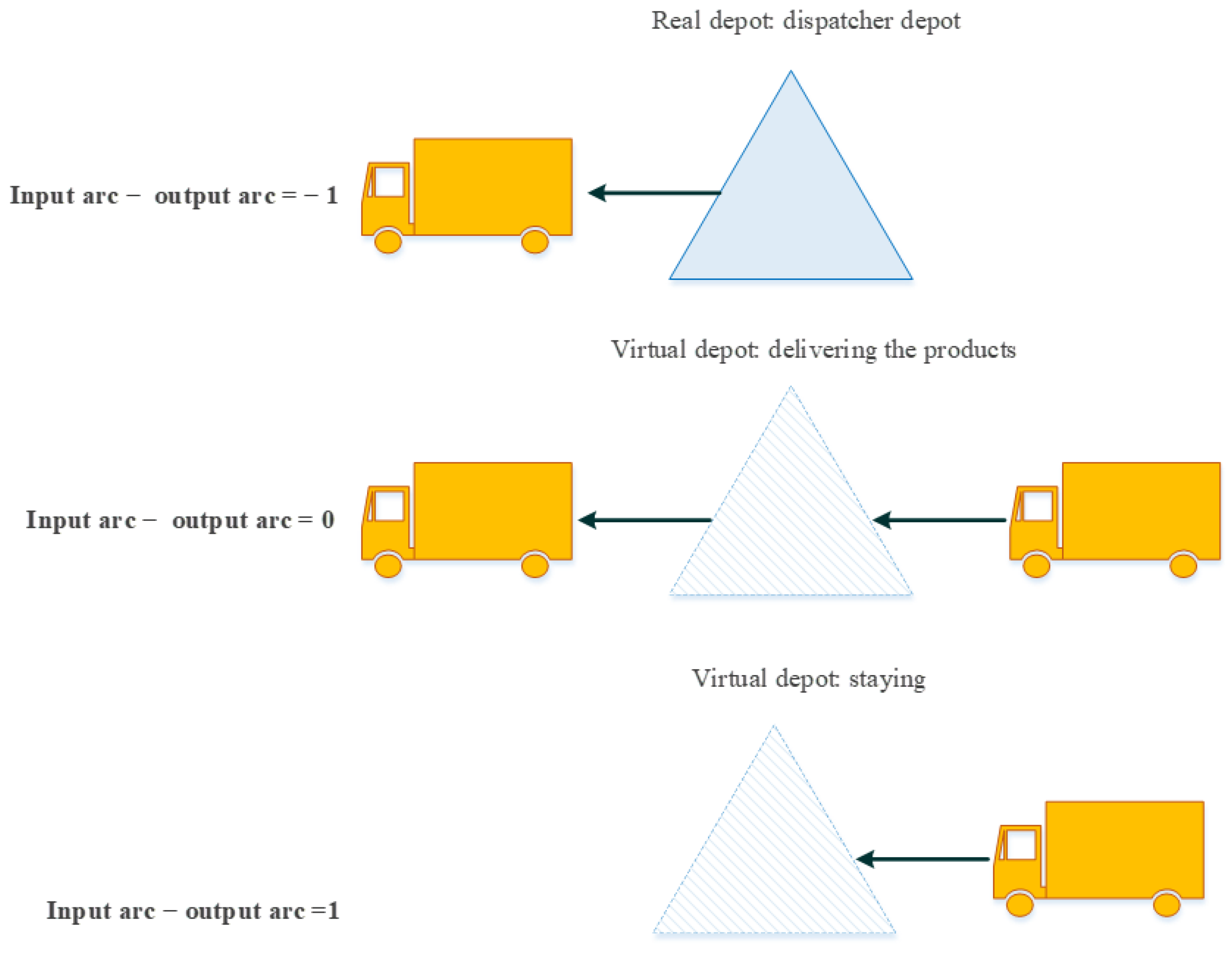
The distance of each virtual depot to its corresponding depot is zero, and the distance to the other nodes of the network (suppliers and other depots) is equal to the distance of its real depot to those nodes;
-
The virtual depot acts as a delivery depot or a staying depot, where a vehicle delivers the purchased products to the depot, or stays at the end of its route. It should be noted that the latter is only possible if the vehicle has already delivered the products of other depots;
-
No vehicles can be dispatched from virtual depots—they can only be dispatched from real depots (if necessary). In fact, real depots just act as dispatchers, and no vehicle is allowed to enter them.
Based on Figure 4, if the flow of a virtual depot (input arc–output arc) is zero, it shows that the vehicle has just delivered the purchased products to this depot, and then gone on to buy and deliver products to other depots. However, if the flow of a virtual depot is one, the vehicle stays at that depot at the end of its route (after delivering the purchased products of other depots). However, due to the limited parking space in each depot, the number of vehicles that park in a specific depot cannot exceed a certain number. Based on the reformed network in the Multi-Trip, Open Vehicle Routing Problem, all routes (closed or open) are transformed to open routes. Thus, if the final virtual depot of a route corresponds to its initial real depot, the route is closed. Otherwise, it is an open route.

4. Mathematical Modeling

In this section, we model our variant of the MDTPP, denoted as MDTPPSR, and propose a tailored mathematical formulation according to the explained reformed network of MDTPPSR.
The following assumptions are made:
-
The demands of all products are unitary;
-
Each depot has only one vehicle with a limited capacity, and without a loss of generality, the index of each vehicle is equal to the index of its corresponding depot;
-
Each depot has a limited parking space;
-
Each product is supplied by at least one supplier.
The sets, parameters, and decision variables of the model are shown in Table 3.
The mathematical formulation for the MDTPPSR is given as follows:
min ( i , j ) A k K c i j x i j k + p P d   D i I p k K w p , i z p , d , i k
Subject to:
    j i j     V ´ x i j k =     j i j     V ´ x j i k = y i k                               i I   , k K
k K i I p z p , d , i k = 1                           p P   , d D : f p , d = 1
z p , d , i k y i k                       p P   , d D , i I   , k K
h i k = p P d D z p , d , i k               i I   , k K  
h d + | D | k = p P i I p z p , d , i k                     k K   , d D    
h d k = 0                                           k K   , d D
i f   x i j k = 1 L i k + h i k L j k                     i V ´ , j V ´ , i j ,   k K                      
L j k Q k                               j V ´ , k K            
i V ´ x i d k = 0                                       k K   , d D      
j V ´ x d j k = 0                                     k K   , d D : d k          
x d + | D | , d k + x d , d + | D | k = 0                         k K   , d D    
i f       p P i I p z p , d , i k > 0 j V ´ x j , d + | D | k > 0                         k K   , d D      
j V ´ x d j k 1                                   k K   , d D : d = k          
p P d k i I p z p , d , i k       α k × p P d D i I p z p , d , i k                               k K  
u i k u j k + | V ´ | × x i j k | V ´ | 1                             i V ´ , j V ´ , i j ,   k K          
i f   u j k > u d + | D | k z p , d , j k = 0                             j I   , d D   k K   , p P  
j V ´ x j , d + | D | k i V ´ x d + | D | , i k                               d D k K    
s d + | D | k =     j V ´ x j , d + | D | k     j V ´ x d + | D | , j k                             d D , k K                
k s d + | D | k P S d + | D |                                       d D  
x i j k , y i k , p s i k , z p , d , i k   { 0 , 1 } , h i k a n d     u i k   a r e   u r s ,   L i k 0   a n d   i n t i , j V ´ , d D ,   k K , p P
The objective Equation (1) minimizes total costs, including purchasers’ total transportation and purchasing costs. Equation (2) is a degree constraint where, if vehicle k goes to supplier i , two edges (incoming and outcoming ones) must enter this supplier. Equation (3) guarantees that the demands for each purchaser’s products are satisfied. constraint (4) dictates that it not be possible to purchase a product from an unvisited supplier. Equation (5) shows the purchased products of supplier i carried by vehicle k . However, if node i is one of the depot’s nodes, then, based on Equation (6), vehicle k delivers the depot’s corresponding purchased products to its virtual depot. As mentioned before, each depot’s products are delivered to its virtual depot. So, based on Equation (7), the load of vehicle k at the moment of leaving its actual depot (dispatch depot) is equal to zero. Constraint (8) is called the “lifted Miller Tucker Zemlin constraint” [51], which shows the upper bound of the vehicle’s load k at the moment of leaving node i , before entering node j . Constraint (9) shows the vehicle capacity constraint. Constraint (10) shows that a vehicle cannot enter a real dispatch depot (the products are delivered to virtual depots). Equation (11) shows that a vehicle can exit a depot only if it belongs to its corresponding depot. It is assumed that each vehicle has the same index as its depot, so obviously, if the vehicle’s index is different from the depot’s index, the vehicle cannot start its route from that depot. Equation (12) indicates that it is not possible to move between the delivery node (the virtual node) and the dispatching node (real node) of a depot. Constraint (13) ensures that the purchased products of each depot are delivered to its virtual delivery depot. Constraint (14) shows that, in the collaborative framework, contrary to the classic TPP, there is no need to dispatch each vehicle from its depot, and a depot (purchaser) can receive its purchased products from other purchasers’ vehicles. Constraint (15) indicates the threshold limit for each purchaser to collaborate with others; in fact, the number of loadings of other purchasers’ products could be, at most, as much as the rate of the total purchasing, shown by α k . It should be noted that in the case of partial collaboration ( α k < 1 ), this constraint inexplicitly imposes a limitation on the number of the purchased products of depot k that are loaded by its vehicle (vehicle k ). In other words, it is impossible for vehicle k to load the products of other depots without loading any product of its depot. Therefore, underutilization is no longer an issue with this restriction. While preventing the creation of a subtour for each vehicle, Constraint (16) specifies the order in which the nodes will be traversed by vehicle k by defining Constraint (17). Given that each vehicle is allowed to visit each node at most once, according to constraint (17), if vehicle K enters supplier j while visiting delivery depot d + | D | earlier ( u j k > u d + | D | k ), it is not allowed to purchase the products of depot d . Otherwise, it has to revisit depot d + | D | to deliver its products. Constraint (18) indicates that it is not possible for a virtual delivery depot to have only one outgoing edge, without any incoming ones. There are only dispatcher depots (real depots) that have one outgoing edge without incoming ones. Equation (19) refers to the staying at or passing on from a specific depot (virtual ones). Here, if the right-hand side value of this equation is zero, it shows that the vehicle has just passed by that depot, and if it is one, the vehicle has stayed at that depot, and parked there. Constraint (20) shows the parking space limitations of each depot. Finally, Equation (21) shows the domain of each variable.
The above Constraint (8), (13), and (17) are logical constraints. Equation (8) is converted to its linear equivalent formulation based on Equation (22).
L i k + h i k + M x i j k M + L j k                                   i V ´ , j V ´ , i j ,   k K  
Equation (13) is linearized based on Equations (23) and (24).
p P i I p z p , d , i k p w p , d × δ d k                                       k K   , d D  
j V ´ x j , d + | D | k δ d k 0                                     k K   , d D              
In the above formulation,   δ d k is a binary variable.
Finally, Equation (17) is converted to its linear form based on the following equations:
u j k u d + | D | k M ´ × O j , d k 0               j I   , k K   , d D , p P : f p , d > 0            
z p , d , j k 1 O j , d k                                 j I   , k K   , d D , p P  
Similarly, in the above equation,   O j , d k is a binary variable that was used for linearization.   M ´ is an upper bound of u j k u d + | D | k .

5. The Proposed Heuristic Algorithm for the MDTPPSR

The MDTPPSR reduces to the classical TPP. In fact, if the α k in the model is set to zero, our proposed problem is converted to multiple depots that purchase their products independently. As the TPP is NP-hard, so is our proposed problem. Undoubtedly, due to the collaboration structure between different purchasers, this problem is far more complex than the typical TPP. One specific feature of the MDTPPSR is that the subsets of collaborative purchasers are not determined beforehand. In fact, in a network with n depots (purchasers), the total number of possible collaborations between depots is an order of O(n 2 n ) (Equation (27)):
[ C ( n , 1 ) + C ( n , 2 ) + + C ( n , n ) ] = 2 n 1
In the following, we propose a decomposition-based algorithm that breaks down the problem based on its specific structure into two manageable pieces, in order to tackle this complexity.

5.1. Decomposition Algorithm

Given the complexity of this problem, we develop a decomposition-based structure with two phases. We state the phases in the context of full collaboration ( α k   = 1), and then present some equations related to a case of partial collaboration ( α k   < 1) in Section 7. In the full collaboration structure, the vehicle of a specific depot can load the products of other depots even without loading any products of its depot. The two phases of the proposed algorithm are given below.
Phase 1—Allocating products to suppliers and vehicles:
In this phase, the supplier of each product, and the product’s carrier, are determined based on Equation (28).
m i n i I { p r i c e p , i + m i n d D ( d i s t a n c e d , i ) }                 p P  
subject to:
p P i I x p i d c a p a c i t y d                 d D      
where x p i d is a binary variable representing whether product p is purchased from supplier i and carried by the vehicle of depot d   or not. As can be seen, for each product, supplier selection and carrier assignment are performed concurrently based on the product’s minimum price, and the minimum distance of the corresponding supplier to the depots. The product’s carrier is the vehicle of the depot that allows the minimum cost in Equation (28). Based on Equation (29), the total number of products purchased from different suppliers depends on the capacity of the vehicle to which the products are assigned.
Phase 2—Routing:
In the second phase, a routing problem is solved. In this VRP, in addition to typical VRP constraints, the capacity constraint and delivery of the products to each corresponding depot should be considered. Moreover, the related suppliers of each depot should be visited before this depot. Additionally, depending on whether or not the final depot of a route is similar to its initial counterpart, the route of a vehicle is a closed routing or a Multi-Trip, Open Vehicle Routing Problem.
Assuming this problem is a particular extension of the VRP, there are three types of nodes: starting depot, suppliers, and delivery depots. The first one is the depot whose vehicle loads the purchased products (obtained from phase 1). The suppliers are equivalent to customer nodes in the classical VRP with positive demands (the demand of each supplier node is the sum of products purchased from it (in phase1)). Finally, the delivery depots correspond to customers with negative demands (the negative demand of each delivery depot is the sum of products that should be delivered to this depot (with a negative sign)). If the initial depot is not a delivery depot, the vehicle route is an open route. By assuming the total number of depots as | D | , the number of allocations ( | R | ) in phase 1 would be 1 | R | | D | . For each allocation, the routing problem is solved as follows.
Since the starting depot may be a delivery depot, we define a virtual starting depot whose distance from each node is the same as that from the starting depot to others. Therefore, with this virtual node, all routes are considered as open routes. (The virtual depot is just a dispatcher depot, and all products are delivered to the delivery depot.)
The sets, parameters, and decision variable of the model in phase 2 are shown in Table 4.
Considering Table 4, the mathematical model of the routing problem is given based on Equations (30)–(37), as follows:
min i , j c i j x i j
subject to
i j x i j = i j x j i = 1                                       j I    
i d x i d = 1                     d D
j d x d j 1                                     d D
i S i j x i j     Q                             i , j T
u i u j + | T | × x i j | T | 1                             i T , j T , i j , i > = 2          
u i m i n i m u m ( u d : ( d , i ) > 0 )                                   i I      
x i j { 0 , 1 } ,   u i   i s   u r s                                               i , j T
Objective Equation (30) minimizes the transportation cost. The degree constraint in Equation (31) ensures that each supplier is visited at phase 1. Equation (32) indicates that the products of each depot are delivered. Constraint (33) guarantees that each delivery node can have at most one outgoing arc. Constraint (34) guarantees that the vehicle capacity constraint is satisfied. Constraint (35) determines the visit sequence of each node. Constraint (36) ensures that suppliers are visited before their corresponding depots. Finally, Equation (37) shows the domains of variables.

5.2. Improvement Heuristics

As described in phase 1, the tactical decisions regarding supplier selection and collaborative purchasers are based on Equation (28). However, leaving out decision-making about routing does not guarantee that Equation (28) leads to the best selection. Thus, in this section, we propose two types of heuristic algorithms to revise and improve the decisions made in phase 1.
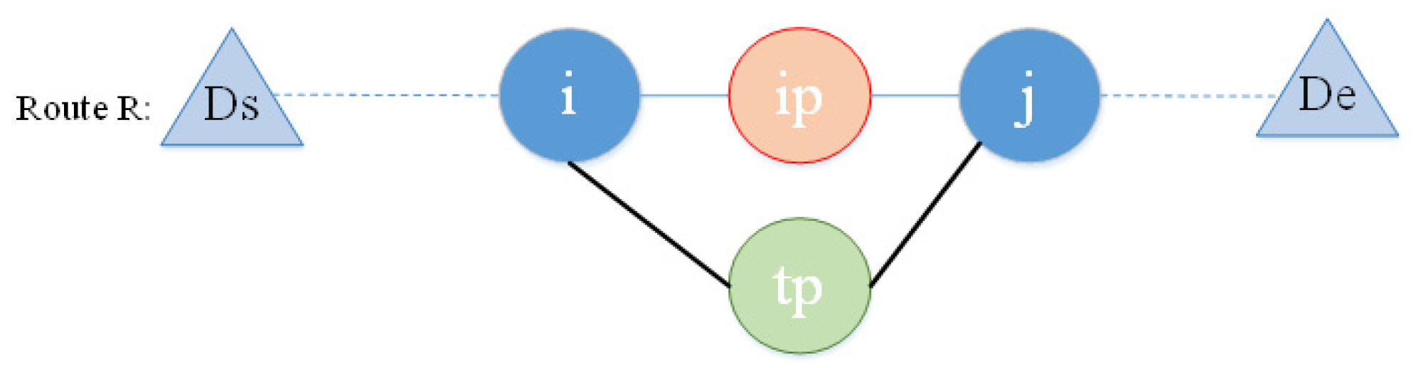
  • Heuristic approach for selected suppliers—in this algorithm, we replace the supplier of each product with another supplier of that product, resulting in maximum saving. Consider route r in Figure 5.
Figure 5. The position of supplier i p in route R ( i p : selected supplier, t p : substitute supplier, D s : start depot, D e : end depot).
Sustainability 14 10190 g005
Consider t p as a substitution for i p ( t p is another supplier of product p ). The saving of this substitution ( t p ) is calculated as follows:
t p = d i s t a n c e ( i , t p   ) + d i s t a n c e ( t p   , j ) + p r i c e t p d i s t a n c e ( i , i p   ) d i s t a n c e ( i p , j   ) p r i c e i p
We exchange supplier i p with a supplier with the minimum negative m i n i p .
m i n i p = min { j | j S p   a n d   j < 0 }
where S p is the set of suppliers of product p . The current supplier of product p ( i p ) is replaced by the corresponding supplier of m i n i p .
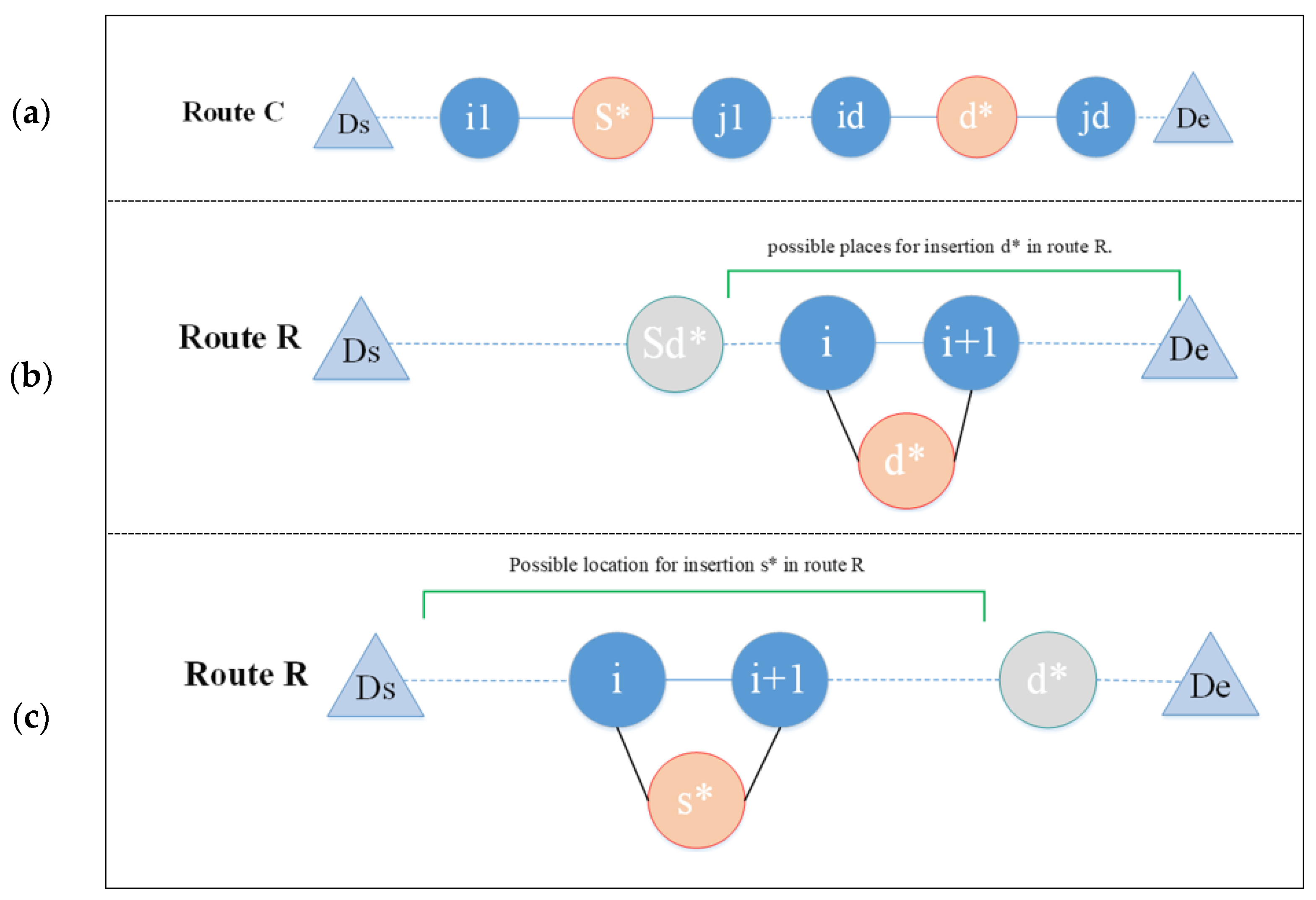
  • Heuristic approach for assigning products to the vehicles of the other depots—as mentioned earlier, in the case of assigning a product to a depot’s vehicle, a better assignment (supplier assignment to a depot’s vehicle) might be set. So, this heuristic algorithm tests the reassigning of the suppliers of products to a route with less transportation costs. It is clear that the purchasing cost is not changed by changing the position of a particular supplier on another route.
Without a loss of generality, the intended supplier (the supplier that is going to be relocated to another route), and its corresponding product and depot, are denoted by s * ,   p * , and d * , respectively. Moreover, for simplicity, we call the current route of the supplier s *   C , and consider the optional route (the route where s * is going) as route R . There are four different scenarios for s * , as determined by the positions of s * and d * in the current route (route C), and the possible places for inserting s * or d * into optional route R, as shown in Figure 6.
  • Scenario 1: supplier s * and its corresponding depot d * ae present on the optional route R .
In this case, the supplier s * on route R is the supplier of other products (except for product p * ), and some other products of depot d * are supplied on the optional route R . Therefore, there is no need to find the locations of s * and d * on route R .
It is clear that, if on the current route C , supplier s * supplies the product(s) of depot d * , and if other products besides product p * are purchased on C , route C undergoes no change, and, thus, the saving cost is zero.
Generally, considering Figure 6a, the saving in transportation cost is calculated as follows:
t p = θ s * [ d i s t a n c e ( i 1 , j 1 ) d i s t a n c e ( i 1   , s * ) d i s t a n c e ( s * , j 1 ) ] + θ d * [ d i s t a n c e ( i d , j d ) d i s t a n c e ( i d   , d *   ) d i s t a n c e ( d *   , j d ) ]
where θ s * and θ d * are binary parameters; θ s * takes a value of 1 if only product p * is supplied by the supplier s * (no other products are purchased from the supplier s * on route C ), and, similarly, θ d * takes a value of 1 if only product p * of depot d * is purchased on route C.
  • Scenario 2: supplier s * exists on the optional route R , but its corresponding depot d * does not exist.
Contrary to the first scenario, here, only s * is on the optional route R , and the location of depot d * should be determined on route R . As such, a strategy similar to that presented by [53] for re-optimizing a TSP tour, wherein a node is added to or dropped from an optimized TSP tour, is applied to find a suitable location for d *   here. However, it should be noted that depot d * on route R can only be located in places after its corresponding suppliers (suppliers from which the products of depot d * are purchased). Let s d * be the last supplier of depot d * on route R . So, based on Figure 6b, the saving cost of inserting depot d * on route R is calculated based on Equation (41).
i : t h e   l o c a t i o n   i   i s   a f t e r   s d *   = d i s t a n c e ( i , d * ) + d i s t a n c e ( d * , i + 1 ) d i s t a n c e ( i , i + 1 ) - θ s * [ d i s t a n c e ( i 1 , j 1 ) d i s t a n c e ( i 1   , s * ) d i s t a n c e ( s * , j 1 ) ] θ d * [ d i s t a n c e ( i d , j d ) d i s t a n c e ( i d   , d *   ) d i s t a n c e ( d *   , j d ) ]
θ s * and θ d * in Equation (41) have the same definitions as Equation (40). The location of depot d * on route R is the one that leads to the maximum cost-savings (Equation (42)).
m i n i = min { i | n o d e   i   i s   a f t e r s d *   i n   r o u t e   R   a n d   i < 0 }
  • Scenario 3: supplier s * is not included on the optional route R, while its depot d * is. In this scenario, the supplier s * can be located before depot d * (Figure 6c).
i : t h e   l o c a t i o n   i   i s   b e f o r e     d *   = d i s t a n c e ( i , s * ) + d i s t a n c e ( s * , i + 1 ) d i s t a n c e ( i , i + 1 ) - θ s * [ d i s t a n c e ( i , j ) d i s t a n c e ( i   , s * ) d i s t a n c e ( s * , j ) ] θ d * [ d i s t a n c e ( i d , j d ) d i s t a n c e ( i d   , d *   ) d i s t a n c e ( d *   , j d ) ]
After calculating the cost-saving for each possible location using Equation (43), the location with the maximum cost-savings is selected for the insertion of supplier s * on route R (Equation (43)).
m i n i = min { i | n o d e   i   i s   b e f o r e   d *   i n   r o u t e   R   a n d   i < 0 }
  • Scenario 4: neither supplier s * nor depot d * exists on route R.
In scenario 4, the locations of both d * and s * should be determined. However, location d * has to be located after the location of s * .
i , j i = 1 2 3 + 4 i n   w h i c h   1 , 2 , 3   a n d   4   a r e   a s   f o l l o w s :
1 = d i s t a n c e ( i , s * ) + d i s t a n c e ( s * , i + 1 ) d i s t a n c e ( i , i + 1 )
2 = θ s * [ d i s t a n c e ( i s , j s ) d i s t a n c e ( i s   , s * ) d i s t a n c e ( s * , j s ) ]
3 = θ d * [ d i s t a n c e ( i d , j d ) d i s t a n c e ( i d   , d *   ) d i s t a n c e ( d *   , j d ) ]
4 = m i n j i : j   i s   a f t e r   i (   d i s t a n c e ( j i , d * ) + d i s t a n c e ( d * , j i + 1 ) d i s t a n c e ( j i , j i + 1 ) )
In scenario 4, the cost saving of inserting s * and d * is shown via Equation (45). In Equation (46), 1 is the distance cost of inserting s * into route R. In 2 (Equation (47)), i s and j s are pre- and post-nodes of s * on the current route C. Similarly, in 3 (Equation (48)), i d and j d are the pre- and post-nodes of d * on the current route C. As can been seen in Equation (49), location i is considered as a potential location for the insertion of supplier s * , and location j (which is after location i ) is suitable for the insertion of depot d * . The distance cost of inserting d * in route R is shown as 4 in Equation (49). Finally, the locations selected for the insertion of s * and d * lead to the maximum reduction in transportation cost.

6. Computational Experiments

In this section, the computational results of different experimental cases are presented to evaluate the performance of the proposed solution algorithm. The test problems were run on Intel Core i3 with 2.30 GHz and RAM 10.00 GB.

6.1. Structure of Instances

There is no specific dataset for our proposed problem (MDTPPSR) in the literature. Thus, the benchmark instances presented by [28] have been modified for our proposed model. In this benchmark, the suppliers’ and depots’ integer coordinates are randomly generated in a [ 0 , 1000 ] × [ 0 , 1000   ] square according to a uniform distribution. Moreover, routing costs are computed by Euclidean distances through the EUC_2D function from TSPLIB [54]. The product’s demand is unitary [28].
After calculating the distance matrix of n city, | D | different points from the | V | points are randomly selected as the depots. Each product k is randomly associated with | S k | selected suppliers, where | S k | is randomly generated in the interval [ 1 , | S |   ] . For each product k and each supplier i , the prices p i k are selected in the interval [ 1 , 200   ] according to a discrete uniform distribution.
To generate the required products of each depot, without a loss of generality, the members of the total product set P are numbered consecutively from the products of the first depot to the products of the last depot. Let | P | be the total number of products (the products of all depots). In our instance set, we choose   ( | D | 1 ) separators such that the places of these separators are randomly generated in the interval (2,   | P | 1 ) according to a discrete uniform distribution. The products of each subsection (created by the separators) yield the required products of each | D | depot.

6.2. Computational Results

In this part, the proposed heuristic algorithm for the Multi-Depot TPP under Shared Resources is compared to the individual case in which each purchaser performs its purchasing on its own. This is primarily done to compare the cost-savings achieved for whole purchasers by using shared resources. Before this comparison, in order to analyze the function of our proposed heuristic algorithm, some random problems have been generated, and the results are compared with the exact Branch and Cut (B&C) technique of the IBM ILOG CPLEX 12.6 solver [55]. It should be mentioned that CPLEX 12.6 is one of the versions of IBM ILOG CPLEX Optimization Studio that is a well-known commercial optimization software package [56].
The results are shown in Table 5. As can be seen, the proposed algorithms achieve an acceptable performance; in most instances, the gap in the percentage of the CPLEX between our algorithm and B&C is less than 1%. From the perspective of CPU time, our proposed algorithm reaches the optimal (near-optimal) solution in considerably less time. In fact, by increasing the sizes of the problems, the CPU time of B&C technique increases exponentially. Meanwhile, when increasing the sizes of the problems, the B&C cannot reach the solution in a reasonable time. However, our algorithm is capable of finding the solution in an acceptable time. For example, in instance number 7, the time required to reach the near-optimal solution (with an optimal gap of 0.7%) is less than one minute, while this time in the exact method is about two hours.
As mentioned earlier, when increasing the sizes of the problems (especially the number of purchasers), the exact method of CPLEX is not capable of finding the optimal solution. So, in order to compare the results of our proposed collaborative model with the individual case, the performance of the decomposed heuristic-based algorithm (with and also without two improving heuristic algorithms) is compared with multi-independent TPPs. Note that individual cases are solved optimally via CPLEX 12.6.
The computational results are presented in Table 6, where the columns show the problem’s size and its specifications. For example, in V10-d3-s7-p15-park2, the numbers of depots and all suppliers are three and seven, respectively. Therefore, the number of all nodes (depots and suppliers) is 10. p15 refers to the total number of all required products. Finally, park2 means that the parking spaces of each depot are assumed to number two. The column “Phases 1 and 2 (without heuristic)” and “Phases 1 and 2 (with heuristic 1 and 2)” denotes the total cost of all purchasers, calculated from the proposed two-phase decomposition algorithm without and with improving heuristics. As described in Section 5, the MDTPPSR is first solved through two phases, and then, to improve the quality of the solutions, two types of heuristic algorithms are applied to it. In Table 6, the two columns of saving A and saving B refer to the cost-savings of the two phases without and with the implementation of heuristic algorithms. The cost-saving percentage in columns 5 and 7 is calculated as follows:
SH 1 = O F _ M D T P P O F _ M D T P P S R O F _ M D T P P
where SH1 is the total of the heuristic one, and O F _ M D T P P S R and O F _ M D T P P are the objective values of the MDTPPSR and MDTPP, respectively. Note that these cost savings are compared with their corresponding individual cases, whose costs are shown in the last column. Moreover, we calculated the total number of dispatched vehicles in the collaborative structure. Cleary, in individual cases, all vehicles are sent from their depots.
Based on the results, the average cost-saving achieved by phases 1 and 2 (without applying heuristic algorithms) is about 11.96%. Meanwhile, in 69% of instances, the proposed phases 1 and 2 algorithms solely help to reduce the total purchasers’ costs compared to individual cases. However, in some instances, the two-phase algorithm was not able to save cost compared to the classical TPP problem (the equivalent individual forms). However, when applying two types of improvement heuristics, the total cost decreased, and more cost savings were achieved. On average, applying heuristic type one (H1) leads to a 13.70% cost saving. This saving increases up to 16.87% when heuristic type two (H2) is applied. The maximum savings achieved when applying heuristic type one (H1) and type two (H2) are, respectively, 26.42% (case 6) and 29.11% (case 13).
From the data in Table 5, it can be inferred that applying the heuristic H1 to the primary algorithm (the two-phase algorithm) improves the cost-saving percentage by up to 1.6%. However, when the second type of heuristic is applied to the primary algorithm, the improvement is about 8.94%. These results accentuate the importance of choosing suitable collaborator carriers to total purchasers’ costs. In other words, a supplier that used to be visited by the vehicle of a specific purchaser is visited by another purchaser’s vehicle, with the exchange likely affecting the whole structure of collaboration.
Based on the results, it can be concluded that the number of potential collaborators (and equivalently, the number of purchasers) has a remarkable effect on the total saving achieved through collaboration. Figure 7 shows a downward trend in saving percentage with an increase in the number of purchasers. Furthermore, comparing these three solution methods highlights the superior performance of the last solution algorithm (phases 1 and 2 with heuristic H2) regarding total cost-saving.
Another positive aspect of using shared resources is the reduction in the number of dispatched vehicles, which helps to reduce the cost of vehicles (the fixed and operation costs) on the one hand, and protect the environment by emitting fewer pollutants into the atmosphere on the other hand. As can be seen, using about half of the available vehicles is sufficient to enable the purchasing of all the purchasers’ products at a lower total cost (Figure 8).

7. Sensitivity Analysis

A sensitivity analysis has been performed in order to study the behavior of the mathematical model. So, in the first part of this section, we show the effect of collaboration rate on the problem structure, and then in the second part, we present some theoretical analyses for determining the optimal range of the partial collaboration rate. Moreover, we calculate the minimum number of required vehicles in the case of partial collaboration.

7.1. Sensitivity Analysis of the Collaboration Rate

In this section, we try to investigate the behavior of our proposed model by changing the collaboration rate. The problem size is as follows: | V | = 5 , | D | = 2 , | S | = 3 , | P 1 | = 4   , and | P 2 | = 3 . Figure 8 demonstrates how all purchasers’ network costs will change with a decrease in the rate of allowed collaboration between different purchasers.
As the collaboration rate decreases, the feasible solution space is limited, and the total cost increases. However, as shown in Figure 9, an optimal range in the collaboration rate can be considered in the range [ 0.57 ,   1 ] . Thus, if some purchasers resist full collaboration, the central manager can determine a partial collaboration range with the same optimality as the full collaboration. For instance, there might be cases when a certain purchaser is willing to collaborate with other purchasers but not all purchasers, due to strong competition. In other words, in the case of full collaboration, a purchaser’s vehicle might have to carry others’ products, even without carrying one product of its own, likely causing an increase in the purchaser’s dissatisfaction with the collaboration structure. So, as members’ satisfaction is a fundamental factor contributing to the success of every collaboration structure, the central decision-maker should implement a collaboration structure that can satisfy the purchasers; thus, when some purchasers are opposed to full collaboration, the central decision-maker can analyze the sensitivity of the collaboration rate and offer the appropriate range of collaboration.

7.2. The Optimal Range of the Partial Collaboration Rate

As mentioned earlier, clearly, the optimal solution is achieved through full collaboration. However, the optimal range of the collaboration rate that leads to the optimal solution can be achieved by having the optimal answer. For simplicity, the number of the corresponding products of depot k that are carried by vehicle k is shown by Y , and X denotes the products of the other depots that are carried by vehicle k. Additionally, α is the symbol of the collaboration rate of each vehicle. Using Equation (15) in our problem, the lower bound of y 1 1 + y 2 2 can be calculated as follows:
( y 1 1 + y 2 2 ) ( 1 α ) ( | P 1 | + | P 2 | )
y d d is the number of products from depot d   carried by its vehicle. With some calculation, we achieve:
    1 α α   ( x 2 1 + x 1 2 ) ( y 1 1 + y 2 2 )
So, by considering the lower limit of Equation (51), we should derive:
    1 α α     ( x 2 1 + x 1 2 ) ( 1 α ) ( | P 1 | + | P 2 | )
Since the optimal solution is calculated based on full collaboration, clearly, α > 0.5 . By simplifying the above equation, the lower bound of the collaboration rate can be calculated as follows:
    α   ( x 2 1 + x 1 2 ) ( | P 1 | + | P 2 | )
So, in this example, the optimal range of the collaboration rate can be considered to lie in the range [ 0.57 ,   1 ] . Moreover, when the collaboration rate is above 0.57, only one vehicle can load the products of both purchasers. Generally, in a problem with n purchasers and an α collaboration rate, we concluded that the minimum required vehicles can be calculated based on the following formulation (the proof is presented in Appendix A):
    i f   i D :   | P i | 1 α α j ! = i | P j |           t h e   m i n i m u m   r e q u i r e d   v e h i c l e s : 1 E l s e i f   i , j D ,   i j :   | P i | + | P i | 1 α α k ! = i , j | P k |           t h e   m i n i m u m   r e q u i r e d   v e h i c l e s : 2 E l s e i f   i 1 , i 2 , , i T D ,   i u i v   u , v :   s = 1 T | P i s | 1 α α k ! = ( i 1 , i 2 , , i T ) | P k |           t h e   m i n i m u m   r e q u i r e d   v e h i c l e s : T

8. Conclusions and Suggestions for Future Research

In this paper, we present a collaborative structure between different purchasers for the sustainable development of the procurement network. For this purpose, a new variant of the Multi-Depot TPP was presented as a Multi-Depot Travelling Purchaser Problem under Shared Resources (MDTPPSR). In the classical TPP, each purchaser buys its required products individually. Each purchaser might incur extra costs in this independent structure thanks to vehicle underutilization, and additional transportation and purchasing costs. Thus, a new type of TPP wherein multiple purchasers can purchase their products using others’ vehicles is presented in this paper. In our model, the whole network of purchasers is more efficient, and the total cost decreases as well. In this collaborative network, a novel routing problem has been developed as a Multi-Trip, Open Vehicle Routing Problem; according to this problem, despite using shared vehicles, each depot’s vehicle is allowed to park in other depots’ parking spaces without returning to its initial depot. Our proposed model works in the forms of both full and partial collaboration. As the names suggests, in the former case, every form of collaboration is allowed. However, in the latter, a purchaser’s vehicle can load other purchasers’ products only if it loads a portion of its products as well.
Given the highly complex nature of the proposed MDTPPSR, a decomposition-based algorithm has been presented in the case of full collaboration. Then, to improve the quality of the solutions, two types of insertion heuristic algorithms were suggested that amend the decisions made in the decomposition algorithm. The results indicate that applying the decomposition-based algorithm can reduce the total cost by up to 22.81%. Moreover, applying two types of improving heuristic algorithms (H1 and H2) can lead to cost-savings of up to 26.42% and 29.11%, respectively. Moreover, by using shared resources, the number of required vehicles is decreased significantly, which has a great impact on the sustainability of the network of purchasers. In addition, it can be inferred that the number of potential collaborators has a notable effect on the total saving achieved through collaboration; as the number of purchases increases, the total cost saving decreases. It should be noted that partial collaboration is much more complex than full collaboration, and some theoretical formulations for calculating the minimum number of required vehicles have been developed.
As regards future research, various extensions can be suggested. First, since our proposed topic has been presented in a centralized collaborative framework, it seems necessary to find a means for cost allocation among different purchasers. A review of cost allocation methods has been presented in [47], and the interested readers can refer to it.
Another attractive field of research is to consider quantity discount policies offered by potential suppliers. In this way, different purchasers can aggregate their demands to benefit from discounted prices. Fair profit-sharing among buyers can be a strong incentive for buyers to work on collaborative logistics. However, some uncertain changes in the business environment (such as changes in purchasers’ demands or products’ prices) could have negative impacts on joint structure. Therefore, future research could provide a comprehensive model considering the above-mentioned elements.

Author Contributions

Conceptualization, Z.S.H.J.; methodology, Z.S.H.J.; supervision, K.E.; supervision, M.R.; visualization, Z.S.H.J.; writing—original draft, Z.S.H.J., review and editing, T.V.W. All authors have read and agreed to the published version of the manuscript.

Funding

This research received no external funding.

Institutional Review Board Statement

Not applicable.

Informed Consent Statement

Not applicable.

Data Availability Statement

The authors confirm that the data supporting the findings of this study are available upon request.

Conflicts of Interest

The authors declare no conflict of interest.

Appendix A. The Proof of Minimum Required Vehicles in Partial Collaboration

As mentioned in Equation (15), the collaboration structure is determined by:
p P d k i I p z p , d , i k       α k × p P d i I p z p , d , i k                                                 k K          
As mentioned earlier, for simplicity, for each vehicle k (depot k ), the number of corresponding products of depot k carried by vehicle k is shown by Y , and the number of products of other depots carried by vehicle k is denoted by X.
X k α ( X k + Y k ) X k α 1 α   Y k                               k K    
Considering x m k ( m k ) as the number of products of depot m carried by a vehicle of depot k , in a network with three depots, we have the following.
Carrier vehicle—vehicle 1 for depot 1
x 2 1 + x 3 1 α 1 α   y 1 1
Carrier vehicle—vehicle 2 for depot 2
                        x 1 2 + x 3 2 α 1 α   y 2 2
Carrier vehicle—vehicle 3 for depot 3
x 1 3 + x 2 3 α 1 α   y 3 3
By summation of the above equations, we have:
x 2 1 + x 3 1 + x 1 2 + x 3 2 + x 1 3 + x 2 3 α 1 α   (   y 1 1 + y 2 2 + y 3 3 )
Consider the set of P consisting of the products of all depots:
P = { p 1 , p 2 , , p d 1 | P 1 | ,   p d 1 + 1 , , p d 2 | P 2 | , .. , p d n 1 + 1 , , p d n | P n | }
where | P i | is the number of products of depot i ( d i ). We know:
x 1 2 + x 1 3 + y 1 1 = | P 1 | x 1 2 + x 1 3 = | P 1 | y 1 1 x 2 1 + x 2 3 + y 2 2 = | P 2 | x 2 1 + x 2 3 = | P 2 | y 2 2 x 3 1 + x 3 2 + y 3 3 = | P 3 | x 3 1 + x 3 2 = | P 3 | y 3 3
By replacing the above formulations in Equation (A6), the equivalent equation is calculated as follows:
( | P 1 | y 1 1 ) + ( | P 2 | y 2 2 ) + ( | P 3 | y 3 3 ) α 1 α   (   y 1 1 + y 2 2 + y 3 3 )
or
(   y 1 1 + y 2 2 + y 3 3 )   ( 1 α ) ( | P 1 | + | P 2 | + | P 3 | )
Generally, for a problem with n depots, we can conclude Equation (A11):
(   y 1 1 + y 2 2 + + y n n )   ( 1 α ) ( | P 1 | + | P 2 | + + | P n | )
and we thus know that
      y 1 1 | P 1 | ,     y 2 2 | P 2 |           , y n n | P n |
By considering Equations (A11) and (A12), we can calculate the minimum number of required vehicles based on Equation (A13):
    { i f   i D :   | P i | 1 α α j ! = i | P j |           t h e   m i n i m u m   r e q u i r e d   v e h i c l e s : 1 E l s e i f   i , j D ,   i j :   | P i | + | P i | 1 α α k ! = i , j | P k |           t h e   m i n i m u m   r e q u i r e d   v e h i c l e s : 2 E l s e i f   i 1 , i 2 , , i T D ,   i u i v   u , v :   s = 1 T | P i s | 1 α α k ! = ( i 1 , i 2 , , i T ) | P k |           t h e   m i n i m u m   r e q u i r e d   v e h i c l e s : T
As mentioned earlier, in the case of partial collaboration, if a depot’s vehicle is dispatched, it has to carry some of its own depot’s products (Equation (A11)). However, by no means does it suggest that all depots’ vehicles have to be dispatched; based on Equation (A13), in a network with n purchasers intending to collaborate, one vehicle might be able to carry the products of its own depot and those of others.

References

  1. Manerba, D.; Mansini, R.; Riera-Ledesma, J. The traveling purchaser problem and its variants. Eur. J. Oper. Res. 2017, 259, 1–18. [Google Scholar] [CrossRef]
  2. Gansterer, M.; Hartl, R.F. Shared resources in collaborative vehicle routing. TOP 2020, 28, 1–20. [Google Scholar] [CrossRef]
  3. Schmelzer, H.; Bütikofer, S.; Hollenstein, L. Kooperieren? Ja! Aber wie?: Chancen und Herausforderungen bei der Entwicklung einer Kooperationsplattform für urbane Güterlogistik in der Stadt Zürich. Logist. Innov. 2016, 2016, 16–19. [Google Scholar]
  4. NextTrust. What is NextTrust? 2AD. 2018. Available online: https://nextrust-project.eu/ (accessed on 8 August 2022).
  5. Li, J.; Wang, R.; Li, T.; Lu, Z.; Pardalos, P.M. Benefit analysis of shared depot resources for multi-depot vehicle routing problem with fuel consumption. Transp. Res. Part D Transp. Environ. 2018, 59, 417–432. [Google Scholar] [CrossRef]
  6. Gansterer, M.; Hartl, R.F. Collaborative vehicle routing: A survey. Eur. J. Oper. Res. 2018, 268, 1–12. [Google Scholar] [CrossRef]
  7. HasanpourJesri, Z.; Eshghi, K. The Multi-Vehicle Traveling Purchaser Problem with Priority in Purchasing and Uncertainty in Demand. Int. J. Logist. Syst. Manag. 2021, 39, 359–389. [Google Scholar] [CrossRef]
  8. Montoya-Torres, J.R.; Franco, J.L.; Isaza, S.N.; Jiménez, H.F.; Herazo-Padilla, N. A literature review on the vehicle routing problem with multiple depots. Comput. Ind. Eng. 2015, 79, 115–129. [Google Scholar] [CrossRef]
  9. Li, J.; Li, Y.; Pardalos, P.M. Multi-depot vehicle routing problem with time windows under shared depot resources. J. Comb. Optim. 2016, 31, 515–532. [Google Scholar] [CrossRef]
  10. Liu, R.; Jiang, Z.; Geng, N. A hybrid genetic algorithm for the multi-depot open vehicle routing problem. OR Spectr. 2014, 36, 401–421. [Google Scholar] [CrossRef]
  11. Sombuntham, P.; Kachitvichyanukul, V. Multi-depot vehicle routing problem with pickup and delivery requests. In AIP Conference Proceedings; American Institute of Physics: College Park, MD, USA, 2010; Volume 1285, pp. 71–85. [Google Scholar]
  12. European Commission. Guidelines on the Applicability of Article 101 of the Treaty on the Functioning of the European Union to Horizontal Co-Operation Agreements. Available online: https://eur-lex.europa.eu/LexUriServ/LexUriServ.do?uri=OJ:C:2011:011:0001:0072:EN:PDF (accessed on 8 August 2022).
  13. Buijs, P.; Alvarez, J.A.L.; Veenstra, M.; Roodbergen, K.J. Improved collaborative transport planning at dutch logistics service provider fritom. Interfaces 2016, 46, 119–132. [Google Scholar] [CrossRef]
  14. Cruijssen, F.; Bräysy, O.; Dullaert, W.; Fleuren, H.; Salomon, M. Joint route planning under varying market conditions. Int. J. Phys. Distrib. Logist. Manag. 2007, 37, 287–304. [Google Scholar] [CrossRef]
  15. Almeida, C.P.; Gonçalves, R.A.; Delgado, M.R.; Goldbarg, E.F.; Goldbarg, M.C. A transgenetic algorithm for the bi-objective traveling purchaser problem. In Proceedings of the IEEE Congress on Evolutionary Computation, Barcelona, Spain, 18–23 July 2010; pp. 1–8. [Google Scholar]
  16. Lin, C.K.Y. A cooperative strategy for a vehicle routing problem with pickup and delivery time windows. Comput. Ind. Eng. 2008, 55, 766–782. [Google Scholar] [CrossRef]
  17. Gouveia, L.; Paias, A.; Voß, S. Models for a traveling purchaser problem with additional side-constraints. Comput. Oper. Res. 2011, 38, 550–558. [Google Scholar] [CrossRef]
  18. Liu, R.; Jiang, Z.; Fung, R.Y.K.; Chen, F.; Liu, X. Two-phase heuristic algorithms for full truckloads multi-depot capacitated vehicle routing problem in carrier collaboration. Comput. Oper. Res. 2010, 37, 950–959. [Google Scholar] [CrossRef]
  19. Cambazard, H.; Penz, B. A constraint programming approach for the traveling purchaser problem. In Principles and Practice of Constraint Programming; Springer: Berlin/Heidelberg, Gemany, 2012; pp. 735–749. [Google Scholar]
  20. Hernández, S.; Peeta, S.; Kalafatas, G. A less-than-truckload carrier collaboration planning problem under dynamic capacities. Transp. Res. Part E Logist. Transp. Rev. 2011, 47, 933–946. [Google Scholar] [CrossRef]
  21. Kang, S.; Ouyang, Y. The traveling purchaser problem with stochastic prices: Exact and approximate algorithms. Eur. J. Oper. Res. 2011, 209, 265–272. [Google Scholar] [CrossRef]
  22. Sprenger, R.; Mönch, L. A methodology to solve large-scale cooperative transportation planning problems. Eur. J. Oper. Res. 2012, 223, 626–636. [Google Scholar] [CrossRef]
  23. Riera-Ledesma, J.; Salazar-González, J.-J. Solving school bus routing using the multiple vehicle traveling purchaser problem: A branch-and-cut approach. Comput. Oper. Res. 2012, 39, 391–404. [Google Scholar] [CrossRef]
  24. Nadarajah, S.; Bookbinder, J.H. Less-than-truckload carrier collaboration problem: Modeling framework and solution approach. J. Heuristics 2013, 19, 917–942. [Google Scholar] [CrossRef]
  25. Batista-Galván, M.; Riera-Ledesma, J.; Salazar-González, J.J. The traveling purchaser problem, with multiple stacks and deliveries: A branch-and-cut approach. Comput. Oper. Res. 2013, 40, 2103–2115. [Google Scholar] [CrossRef]
  26. Bianchessi, N.; Mansini, R.; Speranza, M.G. The distance constrained multiple vehicle traveling purchaser problem. Eur. J. Oper. Res. 2014, 235, 73–87. [Google Scholar] [CrossRef]
  27. Defryn, C.; Sörensen, K.; Cornelissens, T. The selective vehicle routing problem in a collaborative environment. Eur. J. Oper. Res. 2016, 250, 400–411. [Google Scholar] [CrossRef]
  28. Gendreau, M.; Manerba, D.; Mansini, R. The multi-vehicle traveling purchaser problem with pairwise incompatibility constraints and unitary demands: A branch-and-price approach. Eur. J. Oper. Res. 2016, 248, 59–71. [Google Scholar] [CrossRef]
  29. Angelelli, E.; Mansini, R.; Vindigni, M. The stochastic and dynamic traveling purchaser problem. Transp. Sci. 2016, 50, 642–658. [Google Scholar] [CrossRef]
  30. Lai, M.; Cai, X.; Hu, Q. An iterative auction for carrier collaboration in truckload pickup and delivery. Transp. Res. Part E Logist. Transp. Rev. 2017, 107, 60–80. [Google Scholar] [CrossRef]
  31. Beraldi, P.; Bruni, M.E.; Manerba, D.; Mansini, R. A stochastic programming approach for the traveling purchaser problem. IMA J. Manag. Math. 2017, 28, 41–63. [Google Scholar] [CrossRef]
  32. Fernández, E.; Roca-Riu, M.; Speranza, M.G. The shared customer collaboration vehicle routing problem. Eur. J. Oper. Res. 2018, 265, 1078–1093. [Google Scholar] [CrossRef]
  33. Angelelli, E.; Gendreau, M.; Mansini, R.; Vindigni, M. The traveling purchaser problem with time-dependent quantities. Comput. Oper. Res. 2017, 82, 15–26. [Google Scholar] [CrossRef]
  34. Gansterer, M.; Hartl, R.F.; Salzmann, P.E.H. Exact solutions for the collaborative pickup and delivery problem. Cent. Eur. J. Oper. Res. 2018, 26, 357–371. [Google Scholar] [CrossRef]
  35. Hamdan, S.; Larbi, R.; Cheaitou, A.; Alsyouf, I. Green traveling purchaser problem model: A bi-objective optimization approach. In Proceedings of the 2017 7th International Conference on Modeling, Simulation, and Applied Optimization (ICMSAO), Sharjah, United Arab Emirates, 4–6 April 2017; pp. 1–6. [Google Scholar]
  36. Wang, Y.; Yuan, Y.; Assogba, K.; Gong, K.; Wang, H.; Xu, M.; Wang, Y. Design and profit allocation in two-echelon heterogeneous cooperative logistics network optimization. J. Adv. Transp. 2018, 2018, 4607493. [Google Scholar] [CrossRef]
  37. Bernardino, R.; Paias, A. Metaheuristics based on decision hierarchies for the traveling purchaser problem. Int. Trans. Oper. Res. 2018, 25, 1269–1295. [Google Scholar] [CrossRef]
  38. Vaziri, S.; Etebari, F.; Vahdani, B. Development and optimization of a horizontal carrier collaboration vehicle routing model with multi-commodity request allocation. J. Clean. Prod. 2019, 224, 492–505. [Google Scholar] [CrossRef]
  39. Palomo-Martínez, P.J.; Salazar-Aguilar, M.A. The bi-objective traveling purchaser problem with deliveries. Eur. J. Oper. Res. 2019, 273, 608–622. [Google Scholar] [CrossRef]
  40. Quintero-Araujo, C.L.; Gruler, A.; Juan, A.A.; Faulin, J. Using horizontal cooperation concepts in integrated routing and facility-location decisions. Int. Trans. Oper. Res. 2019, 26, 551–576. [Google Scholar] [CrossRef]
  41. Yang, T.; Wang, W. Logistics Network Distribution Optimization Based on Vehicle Sharing. Sustainability 2022, 14, 2159. [Google Scholar] [CrossRef]
  42. Kang, H.-Y.; Lee, A.H.I.; Yeh, Y.-F. An optimization approach for traveling purchaser problem with environmental impact of transportation cost. Kybernetes 2020, 50, 2289–2317. [Google Scholar] [CrossRef]
  43. Wang, Y.; Zhe, J.; Wang, X.; Sun, Y.; Wang, H. Collaborative Multidepot Vehicle Routing Problem with Dynamic Customer Demands and Time Windows. Sustainability 2022, 14, 6709. [Google Scholar] [CrossRef]
  44. Pradhan, K.; Basu, S.; Thakur, K.; Maity, S.; Maiti, M. Imprecise Modified Solid Green Traveling Purchaser Problem for Substitute Items using Quantum-inspired Genetic Algorithm. Comput. Ind. Eng. 2020, 147, 106578. [Google Scholar] [CrossRef]
  45. Wang, Y.; Assogba, K.; Fan, J.; Xu, M.; Liu, Y.; Wang, H. Multi-depot green vehicle routing problem with shared transportation resource: Integration of time-dependent speed and piecewise penalty cost. J. Clean. Prod. 2019, 232, 12–29. [Google Scholar] [CrossRef]
  46. Cheaitou, A.; Hamdan, S.; Larbi, R.; Alsyouf, I. Sustainable traveling purchaser problem with speed optimization. Int. J. Sustain. Transp. 2021, 15, 621–640. [Google Scholar] [CrossRef]
  47. Wang, Y.; Li, Q.; Guan, X.; Xu, M.; Liu, Y.; Wang, H. Two-echelon collaborative multi-depot multi-period vehicle routing problem. Expert Syst. Appl. 2021, 167, 114201. [Google Scholar] [CrossRef]
  48. Hamdan, S.; Cheaitou, A.; Larbi, R.; Alsyouf, I. Moving toward sustainability in managing assets: A sustainable travelling purchaser problem. In Proceedings of the 2018 4th International Conference on Logistics Operations Management (GOL), Le Havre, France, 10–12 April 2018; pp. 1–5. [Google Scholar]
  49. Wang, Y.; Ma, X.; Li, Z.; Liu, Y.; Xu, M.; Wang, Y. Profit distribution in collaborative multiple centers vehicle routing problem. J. Clean. Prod. 2017, 144, 203–219. [Google Scholar] [CrossRef]
  50. Roy, A.; Gao, R.; Jia, L.; Maity, S.; Kar, S. A noble genetic algorithm to solve a solid green traveling purchaser problem with uncertain cost parameters. Am. J. Math. Manag. Sci. 2020, 40, 17–31. [Google Scholar] [CrossRef]
  51. Liu, R.; Jiang, Z. The close–open mixed vehicle routing problem. Eur. J. Oper. Res. 2012, 220, 349–360. [Google Scholar] [CrossRef]
  52. Azadeh, A.; Farrokhi-Asl, H. The Close–Open Mixed Multi Depot Vehicle Routing Problem Considering Internal and External Fleet of Vehicles. Transp. Lett. 2019, 11, 78–92. [Google Scholar] [CrossRef]
  53. Archetti, C.; Bertazzi, L.; Speranza, M.G. Reoptimizing the traveling salesman problem. Networks 2003, 42, 154–159. [Google Scholar] [CrossRef]
  54. Reinhelt, G. {TSPLIB}: A Library of Sample Instances for the TSP (and Related Problems) from Various Sources and of Various Types. 2014. Available online: http//comopt.ifi.uniheidelberg.de/software/TSPLIB95 (accessed on 8 August 2022).
  55. I.A.P.S.A. AP14-0427. IBM ILOG CPLEX Optimization Studio V12.6.1 Delivers Better Performance and a New Licensing Option. Available online: https://www.ibm.com/common/ssi/ShowDoc.wss?docURL=/common/ssi/rep_ca/7/872/ENUSAP14-0427/index.html (accessed on 8 August 2022).
  56. Anand, R.; Aggarwal, D.; Kumar, V. A comparative analysis of optimization solvers. J. Stat. Manag. Syst. 2017, 20, 623–635. [Google Scholar] [CrossRef]
Figure 1. Vehicle loading in individual and collaborative cases ((a) is related to purchasing and loading products individually; (b) is related to purchasing and loading products collaboratively; (c) is the legend of Figure 1).
Sustainability 14 10190 g001
Figure 2. The vehicle routes of each depot in the individual case.
Sustainability 14 10190 g002
Figure 3. The vehicle routes set out via two approaches. (The red route: the route of the empty vehicle). ((a) is related to first approach; (b) is related to second approach).
Sustainability 14 10190 g003
Figure 4. The input and output flows of depots (real and virtual).
Sustainability 14 10190 g004
Figure 6. The schematic view of positions of s * and d * (a) the current position of s * and d * in the route C; (b) the possible places for insertion d* in route R in scenario 2; (c) the possible places for insertion s* in route R in scenario 3.
Sustainability 14 10190 g006
Figure 7. A comparison of the average cost-savings for different sizes of purchasers.
Sustainability 14 10190 g007
Figure 8. The proportion of dispatched vehicles in shared resource cases for different numbers of purchasers.
Sustainability 14 10190 g008
Figure 9. Sensitivity analysis with changing collaboration rate.
Sustainability 14 10190 g009
Table 1. Summarized literature review.
Collaborative VRPTPP
ReferenceLTLFTLObjectiveCost Allocation AllocationCase StudyMethodologyReferenceCollaborationDepotDeterministicUncertainObjectiveUnitary DemandNon-Unitary DemandSingle VehicleMulti Vehicle
[14] cost Empirical analysis[15] single Bi-objective (travel distance and purchasing cost)
[16] cost Heuristic algorithm[17] single Total cost
[18] minimizing empty vehicle movements Heuristic algorithms[19] single Total cost
[20] cost Exact algorithm[21] single Expected total cost
[22] cost Heuristic algorithms[23] single Total cost
[24] cost Heuristic algorithms[25] single Total cost
[13] costHeuristic algorithms[26] single Total cost
[27] cost Heuristic algorithms[28] single Total cost
[9] cost Hybrid metaheuristic algorithm[29] single Total cost
[30] costHeuristic algorithms[31] single Total cost
[32] cost Exact algorithm[33] single Total cost
[34] cost Exact algorithm[35] single Bi-objective (total cost and CO2 emissions)
[36] costHybrid metaheuristic algorithm[37] single Total cost
[38] costHybrid metaheuristic algorithm[39] single Bi-objective (total cost and waiting time of customers)
[40] cost A hybrid metaheuristic algorithm[7] single Total cost
[41] cost Metaheuristic algorithm[42] single Cost (assigning cost, traveling cost and purchasing cost, emission cost, earliness and tardiness)
[43] cost Hybrid metaheuristic algorithm[44] single Total cost with hard constraint on maximum emission level
[45] minimizing total carbon emission and operating cost Hybrid heuristic algorithm[46] single Minimizing total cost, Co2 emission and maximizing total sustainability value
[47] Minimizing operational cost and service timeHybrid heuristic algorithm[48] single Minimizing total cost and maximizing total sustainability score
[49] minimizing the total network costsMulti-phase hybrid approach[50] single Minimizing cost by considering the environmental impact
This paper cost Heuristic algorithmsThis papermultiple Total collaborative cost
Legend for the columns of Collaborative VRP. LTL (less than truckload), FTL (full truckload), Objective (the main focus or the objective function), Cost allocation (allocating the total cost between the members of collaboration in a collaborative VRP), Methodology (the type of solution method for solving the proposed model). Legend for the columns of TPP. Collaboration (a collaboration structure between different purchasers in a Multi-Depot TPP), Unitary demand (the demand for each required product of the purchaser is only one unit), Non-unitary demand (the demand for each required product of the purchaser is more than one), Single vehicle (there is only one vehicle in the depot of the purchaser), Multi vehicle (there are multiple vehicles in the depot of the purchaser).
Table 2. A comparison of collaborative frameworks in terms of inbound and outbound logistics.
Basis FeaturesCollaborative Inbound Logistics (CIL)Collaborative Outbound Logistics (COL)
CollaborationProduct’s Demand AggregationOrder Exchange
Final DeliveryPurchaserCustomer
DimensionMulti-ProductsSingle Product
InteractionDifferent Potential Suppliers and PurchasersKnown Set of Customers and Distributors
Potential OpportunitiesResource Sharing and Group PurchasingResource Sharing
Table 3. The set, parameters, and decision variables for the MDTPPSR model.
Set
A The set of arcs
D , d The set and index of depots (Each depot corresponds to a certain purchaser) ( | D | : number of depots)
I The set of suppliers ( | I | : number of suppliers)
K , k The set and index of purchasers’ vehicles
P , p The set and index of all purchasers’ products
V The set of real network nodes ( V = D   I )
V ´ The set of all nodes in the network (including suppliers, depots, and virtual depots, | V ´ | =2 × | D | + | I | )
Para-meters
α k The allowed collaboration rate between depots ( α k [ 0 , 1 ] )
c i j The traveling cost between two nodes i and j ( i , j V )
f p , d The demand for product P of depot d
P S d The number of parking spaces of depot d
Q k The capacity of vehicle k
w p , i The purchasing cost of product p ( p P ) from supplier i ( i I )
Decisionvariables:
h i k The number of loadings (unloadings) of vehicle k   at the time of visiting node i ( i V ´ ).
L i k The upper limit of the vehicle’s load k when entering node i ( i V ´ ).
s d + | D | k 1, if vehicle k parks at virtual depot d + | D | corresponding to real depot d , 0 otherwise.
u i k An arbitrary variable for subtour elimination in the Miller–Tucker–Zemlin method ( i V ´ ).
x i j k 1, if vehicle k goes from node i to node j , 0 otherwise ( i , j V ´ ).
y i k 1, if supplier i is visited by vehicle k , 0 otherwise ( i I ).
z p , d , i k 1, if product p of depot d is purchased from supplier i by the purchaser’s vehicle k , 0 otherwise.
Table 4. The set, parameters, and decision variable for the routing model.
Set and Parameters
D The set of delivery depots in phase 1
d s The virtual starting depot
I The set of selected suppliers in phase 1
( d , i ) Take value 1 if a product of depot d is purchased from supplier i .
Q The vehicle capacity
S i The demand for node i ( i T ) (the demand for the virtual depot is zero)
T The set of network nodes ( T = I   D   d s )
Decision variables
u i The sequence of visiting node i on the route
x i j 1 if the vehicle goes directly from node i to node j , 0 otherwise
Table 5. Computational results obtained through the proposed heuristic algorithms and the branch and cut method in CPLEX.
RowInstanceHeuristic ResultCPU Time of Heuristic (s)Exact Result of CPLEXCPU Time of CPLEX (s)Optimality Gap (%)
1V10-d3-s7-p15-park24061.437.424046.9413.490.03
2V10-d3-s7-p25-park25025.6517.654980.8325.680.91
3V10-d4-s6-p15-park23871.521.143871.9939.770
4V10-d5-s5-p15-park24971.1247.654971.23421.160
5V10-d5-s5-p25-park26189.0363.086105.386540.261.37
6V11-d5-s6-p15-park24263.7150.644193.266103.781.68
7V11-d6-s5-p15-park25313.4657.135276.536973.130.7
8V12-d5-s7-p15-park24463.9870.344376.454920.372
9V13-d5-s8-p15-park24671.3353.674246.675451.741.01
10V15-d5-s10-p15-park24346.1461.73Out of memory866-
Table 6. Computational results.
RowInstancePhases 1 and 2 (without Heuristic)Number of Dispatched VehiclesSaving A (without Heuristic)Phases 1 and 2 (with Heuristic 1 and 2)Saving B (with Heuristic 1 and 2)Independent Case (Collaboration = 0)
1V10-d3-s7-p15-park24594.42 out of 39.03%H1 + = 4061.11
H2 ++ = 4416.40
SH1 * = 19.60%
SH2 ** = 12.56%
5050.5
2V10-d5-s5-p15-park25170.112 out of 513.20%H1 = 5075.80
H2 = 4971.11
SH1 = 14.78%
SH2 = 16.53%
5956.08
3V10-d5-s5-p20-park25719.62 out of 522.81%H1 = 5713.60
H2 = 5332.69
SH1 = 22.88%
SH2 = 28.02%
7409.36
4V15-d5-s10-p15-park24909.12 out of 5−5.41% *H1 = 4836.30
H2 = 4346.14
SH1 = −3.85% *
SH2 = 6.68%
4657.09
5V15-d5-s10-p25-park29329.535 out of 50.10%H1 = 9280.54
H2 = 7837.82
SH1 = 0.61%
SH2 = 16.07%
9339.13
6V20-d5-s15-p15-park24264.492 out of 525.32%H1 = 4201.50
H2 = 4126.16
SH1 = 26.42%
SH2 = 27.73%
5710.15
7V20-d10-s10-p25-park29302.475 out of 109.30%H1 = 9266.47
H2 = 8112.27
SH1 = 9.65%
SH2 = 20.90%
10,256.65
8V25-d10-s15-p25-park27512.265 out of 109.44%H1 = 7512.26
H2 = 6397.76
SH1 = 9.44%
SH2 = 22.87%
8295.14
9V25-d10-s15-p35-park28920.155 out of 101.17%H1 = 8920.10
H2 = 7821.83
SH1 = 1.17%
SH2 = 13.34%
9026.05
10V25-d5-s20-p20-park24523.683 out of 5−1.98% *H1 = 4235.23
H2 = 4068.62
SH1 = 4.51%
SH2 = 8.27%
4435.67
11V30-d10-s20-p25-park28873.245 out of 10−9.99% *H1 = 6094.34
H2 = 8691.45
SH1 = 24.45%
SH2 = −7.73% *
8067.68
12V30-d10-s20-p40-park214,090.227 out of 10−18.48% *H1 = 14,041.01
H2 = 11,619.46
SH1 = −18.06% *
SH2 = 2.30%
11,892.48
13V35-d10-s25-p20-park25436.024 out of 1021.53%H1 = 5353.12
H2 = 4911.17
SH1 = 22.73%
SH2 = 29.11%
6927.85
14V35-d5-s30-p20-park24018.293 out of 514.14%H1 = 3990.69
H2 = 3910.78
SH1 = 14.73%
SH2 = 16.44%
4680.12
15V30-d15-s15-p20-park29546.9710 out of 155.55%H1 = 9380.82
H2 = 7440.36
SH1 = 7.19%
SH2 = 26.38%
10,107.45
16V35-d15-s20-p30-park212,556.98 out of 15−22.05% *H1 = 12,443.30
H2 = 9691.02
SH1 = −20.94%
SH2 = 5.81%
10,288.3
The negative sign in column 5 shows there is no saving in total cost. +: Total cost from heuristic one (changing supplier with another supplier); ++: Total cost from heuristic two (changing the route of a supplier); *: Saving derived from heuristic one (compared to individual case); **: Saving derived from heuristic two (compared to individual case).
Publisher’s Note: MDPI stays neutral with regard to jurisdictional claims in published maps and institutional affiliations.

