A Hesitant Fuzzy Method for Evaluating Risky Cold Chain Suppliers Based on an Improved TODIM

Abstract

Enterprises need sustainable development in order to reduce costs and increase income. The cold chain logistics industry needs to promote sustainable supply chains more. As the beginning of the supply chain, the choice of suppliers is particularly important. Considering the risky attitude of decision-makers, an improved hesitant fuzzy TODIM approach is adopted to select suppliers. In order to calculate a more objective indicator weight, the generalized Shapley function of the hesitant fuzzy measure is adopted by analyzing the relationships among indicators. The uncertain supplier evaluation information given by decision-makers is obtained by using hesitant fuzzy information. The improved Interactive and Multi-criteria Decision-Making (TODIM) method based on hesitant fuzzy numbers is used to analyze the psychological behavior of decision-makers under different market prospects and comprehensively rank the candidate suppliers. Finally, a case study of selecting cold chain logistics suppliers is provided to verify the effectiveness and feasibility of the method in this paper.

1. Introduction

In the current economic context, the success of any enterprise should be based not only on its profitability, but also on its contribution to the future development of mankind and the Earth. As a supply chain is an indispensable system for enterprises, adding sustainability considerations to the supply chain has been considered an emerging field requiring systematic research. Enterprises must accept sustainability and implement sustainability in their supply chain as part of a long-term strategy to seek a competitive advantage.

In recent years, consumers’ demand for cold chain products has increased with the improvement of people’s material living standards. Dairy products, seafood, fruit, and other cold chain products have increasingly become a part of people’s daily lives.

Since 2015, the cold chain product industry has entered the “Internet era”, and with the development of modern logistics, the relationship between enterprises in the supply chain has gradually evolved from the traditional buying and selling relationship to a cooperative relationship. The difference between this cooperative relationship and the traditional cooperative relationship is that the objectives of all cooperating parties are the same, and all parties who are cooperating have their own interests to consider. Therefore, in order to achieve cooperation, production enterprises not only have strict requirements for the high standards of the products provided; the products should also meet the personalized needs of customers. At present, China’s cold chain logistics system is in the stage of rapid development. In order to make the services of cold chain logistics suppliers meet the requirements of cold chain product manufacturers and their customers, it is very necessary for enterprises and customers to cooperate to select cold chain logistics suppliers.

The cold chain supply chain is a systematic process. All kinds of perishable products have different requirements for harvest time, temperature, humidity, and other conditions. In addition, for the whole supply chain, there are many enterprises involved in its circulation. The selection and evaluation of suppliers have important theoretical and practical significance for the survival and development of enterprises. Supplier selection is mostly a multi-attribute decision-making problem. Through reviewing the previous research, different multi-attribute methods are used to evaluate and select suppliers, such as the Analytic Hierarchy Process (AHP) [1], the Technique Order Preference by Similarity to Ideal Solution (TOPSIS) [2] method, Vlsekriterijumska Optimizacija I Kompromisno Resenje (VIKOR) [3], and the mixed multi-attribute decision-making method [4,5,6] considering uncertain information processing, etc. However, the above supplier selection methods do not consider the market risk factors and the risk attitudes of the decision-makers. The evaluation value of each indicator of candidate suppliers is static and has no relation to the market prospect and other factors. In addition, these methods assume that the decision-maker is completely rational and takes advantage of the expected utility theory. However, in general, decision-makers do not always pursue the maximum utility in their behaviors but choose the solution that makes them satisfied; that is, decision-makers are bounded rational agents. Kahneman and Tversky [7,8] put forward the prospect theory considering the psychological behavior of decision-makers, which has been widely used to solve various multi-attribute decision-making problems. Dai et al. [9] proposed a multi-stage multi-attribute decision-making method based on the prospect theory and the triangular fuzzy multiple objective optimization of full multiplication proportional analysis (MULTIMOORA). Li et al. [10] proposed an approach for the selection of third-party reverse logistics providers based on hybrid-information multi-criteria decision-making (MCDM) and cumulative prospect theory. However, there is no direct data connection between utility and selection in the analysis with the prospect theory. Gomes and Lima [11] proposed the Interactive and Multi-criteria Decision-Making (TODIM) method, which has been widely studied and applied in the field of multi-attribute decision making. Tian et al. [12] proposed a novel TODIM method combined with probabilistic hesitant fuzzy information and applied it in green supplier selection. Liu et al. [13] considered decision-makers’ bounded rationality and vagueness of judgements. Based on the rough set theory, the TODIM method is proposed. Li et al. [14] provide a risk decision analysis method based on the TODIM method. This method directly selects the index values of other alternative schemes as a reference point, which can make the decision-making process more convenient and objective [15]. Therefore, the TODIM method is used to sort the suppliers.

In the decision-making process of supplier selection, due to the complexity and uncertainty of things, as well as the limitations of decision-makers, decision-makers are more inclined to evaluate using uncertain information. In the decision-making process of supplier selection, due to the complexity and uncertainty of things, as well as the limitations of decision-makers, decision-makers are more inclined to evaluate using uncertain information. The traditional TODIM methods typically use accurate numerical values to evaluate indicators. Fuzzy set theory is often adopted to deal with uncertain information, but it relies too much on subjective experience and has the drawback of computational complexity. For the uncertain decision-making environment, the idea of the fuzzy set has been used in the TODIM method [16,17,18]. Based on hesitant fuzzy sets, there has been a wide range of research on, as well as applications of, the decision-making method based on the hesitant fuzzy set (HFS) in recent years. The biggest feature of HFS is that it allows different evaluation values to appear at the same time in a single indicator, which can not only effectively reflect the opinions of decision-makers, but also reflect the decision makers’ hesitation. Therefore, to some extent, hesitant fuzzy sets are more flexible and natural in dealing with uncertain information [19]. In the actual decision-making process, decision-makers often use hesitant fuzzy numbers instead of hesitant fuzzy sets to express their preference information. Compared with traditional fuzzy numbers and intuitionistic fuzzy numbers, hesitant fuzzy numbers allow organizations or individuals to give multiple possible values, increasing the flexibility of assignment and enabling a more detailed description of the uncertainty of things [20,21]. In this paper, hesitant fuzzy and TODIM methods are combined to analyze the psychological preferences of decision-makers. Therefore, hesitant fuzzy and TODIM methods are combined to analyze the psychological preferences of decision-makers.

When calculating the perceived value function in the TODIM method, the index weight needs to be considered. The traditional method for calculating index weight calculation is subjective and given by experts. It does not consider the interrelationship among the indicators. The indicators are complementary. For example, when selecting the supplier of excavator rescue and on-site maintenance, service cost, service efficiency and service quality are usually considered. Usually, the efficiency and quality of the service with lower charges will be relatively low; efficiency conflicts with cost. The indicator weights will be inaccurate without considering the interrelationships among indicators [22]. The additivity rigid constraint in classical probability is replaced by the fuzzy measure with the monotonicity and continuity of weak constraint conditions, which can effectively describe any interaction among the indicators [22]. The fuzzy measure has been used to analyze the influence relationship among indica-tors [23,24]. In this paper, the hesitant fuzzy generalized Shapley function based on the fuzzy measure is used to calculate the index weight that can reflect the mutual influence among indicators.

In this paper, a risky supplier selection method based on the hesitant fuzzy generalized Shapley function is adopted. Firstly, the evaluation index system for cold chain logistics suppliers is constructed. Secondly, the hesitant fuzzy set is used to standardize the evaluation value of suppliers given by experts. Thirdly, considering the mutually influential relationship among the indicators, the generalized Shapley function based on the hesitant fuzzy measure is adopted to analyze the mutually influential relationship among indicators. Finally, considering the risk attitudes of decision-makers, the TODIM method is used to capture the psychological behavior of decision-makers and rank the candidates. Three psychological behavioral preferences are shown by decision-makers in the face of risks: risk aversion, risk neutrality, and risk preference. The effectiveness of this method is illustrated by the selection of a cold chain logistics supplier.

The structure of this paper is shown as follows. Section 1 introduces the background of the cold chain for supplier selection and the causes of the fuzzy hesitant TODIM methods. Section 2 reviews the dependent literatures of cold chain for supplier evaluation and the comparison of the multi-attribute decision-making methods. Section 3 constructs the evaluation index system for cold chain logistics suppliers. Section 4 determines the index weight based on fuzzy measure. Section 5 proposed the integrated fuzzy hesitant Shapely-TODIM method. In Section 6, a case study of selecting cold chain logistics suppliers is provided to verify the effectiveness and feasibility of the method. Section 7 gives the managerial implications, research summary, the limitations, and research prospects.

2. Relevant Literature

2.1. Cold Chain Supplier Evaluation

The cold chain logistics system has higher requirements and is more complex than the general logistics system, and the construction investment is much larger. Researchers have paid a great deal of attention to the cold chain logistics system in recent years. Weng et al. [25] analyzed the development and the trend of the cold chain logistics system. Li. [26] proposed the development of the cold chain logistics transportation system based on 5G network and Internet of things system. However, there is limited research literatures on supplier selection of cold chain logistics. Xiong et al. [27] evaluated the performance of food cold chain logistics enterprises based on the AHP and entropy method. Lau et al. [28] proposed a business process decision model for fresh-food supplier evaluation, thereby taking precautions against the supplier evaluation of the cold chain.

2.2. Common Multi-Attribute Decision-Making Methods

Supplier evaluation is a multi-attribute decision-making process. Common multi-attribute decision-making methods include the Analytic Hierarchy Process (AHP) [29,30,31], the Technique Order Preference by Similarity to Ideal Solution (TOPSIS) method [32,33,34], VIKOR [35,36], DEA [37,38], ELECTRE [39], grey correlation analysis (GCA) [40], and the mixed multi-attribute decision-making method considering uncertain information processing [40,41,42], etc. Different decision-making methods have their own advantages and disadvantages. The comparison of these methods is shown in

Table 1. The Advantage and Disadvantage of Different Decision-making Methods.

Methods	Advantages	Shortcomings
AHP	Decomposes the problem layer by layer, which helps it to be understood and mastered [31]. The consistency can be effectively evaluated.	Needs multiple comparisons, which is cumbersome.
TOPSIS	Refrains from the subjectivity of information [32]. There is no strict limit on the sample’s capacity. It is applicable to large-scale systems with many variables and attributes [34].	The experts have enormous implications for the result [41]. The importance of the distances between ideal points and negative ideal points is not considered.
VIKOR	Maximizes the group utility and minimizes individual regret. The subjective preferences of experts can be effectively expressed [35]. Can provide more than one set of optima solutions out of compromise.	The reasons why some schemes do not meet the conditions cannot be explained [43].
DEA	The evaluation value of each index can be used to provide non-parametric reference values [37]. Can give the reasons why the conditions are not met. The index weight is calculated by a mathematical formula, which is more objective.	The index’s weight obtained through calculation is highly flexible, so it is easy to weaken the differences between the schemes [44]. For the evaluation of schemes, it is only a relative evaluation, not an absolute evaluation.
ELECTRE	The incomplete information can be modeled [45]. Can abate the compensation among indicators.	Just minimizes individual regret. There are defects in dealing with the pure ordinal scale [41]. It is very complicated to calculate the parameters.

.

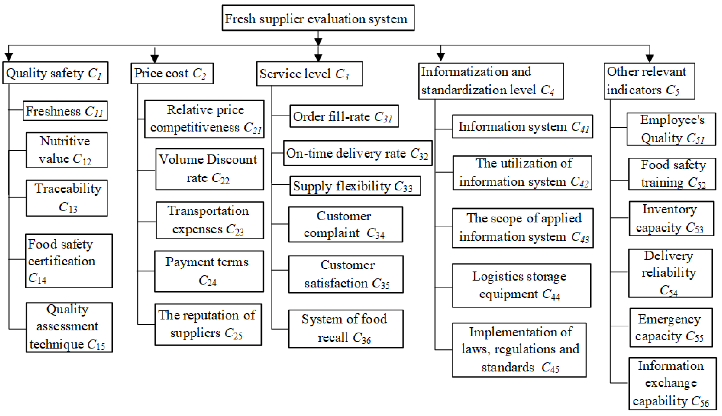
3. Construction of the Evaluation Index System for Cold Chain Logistics Suppliers

The identification and construction of the evaluation index for cold chain logistics suppliers is a very important part of the process of supplier selection and can help decision-makers acquire better decision-making results and provide effective decision results and a basis for the accurate connection of supplier selection. A comprehensive index evaluation system of cold chain logistics suppliers is constructed in Section 2 and includes quality safety, price cost, service level, informatization and standardization level, and other relevant indicators. Every index has a relevant explanation. The interrelationship among attributes is confirmed by relevant literature and experts’ advice. Figure 1 shows the whole scale of evaluation index system for the cold chain logistics supplier. The explanation of each indicator is shown as in

Table 2. Summarizes the evaluation index system for cold chain logistics suppliers.

First-Class Indicators	Second-Class Indicators	Explanation
Quality and safety aspects	Freshness [26,46,47]	The freshness, and the chemical, biological, sensory, and other properties of aquatic products need to meet the standards.
	The nutritive value [27,47]	This refers to the nutrients in food.
	Traceability [28,48]	Food safety can only be guaranteed if food traceability is realized.
	Food safety certifications [25,49]	There are the written guarantees or certificates of conformity given by a third party to the food.
	Quality assessment techniques [47]	Rational quality assessment can make up for the deficiency in quality monitoring.
Price cost aspect	Relative price competitiveness [46]	Price measures are used to compete for market share with competitors.
	The volume discount rate [26,50]	Batch the discount amount as a percentage of the sales price.
	Transportation expenses [46,51]	Transportation expenses that are paid for transporting goods.
	Payment terms [25,51]	A specified discount is promised by the enterprise within a certain period of time.
	The reputation of suppliers [35,46]	The reputation of suppliers mainly depends on the actual performance, rather than advertising or other forms of publicity.
Service level aspect	Order fill-rate [51,52]	It refers to the degree of ability to meet customers’ inventory needs.
	On-time delivery rate [50,52]	The on-time delivery rate is the percentage of on-time deliveries times of lower-tier suppliers out of their total delivery times within a certain period of time.
	Supply flexibility [53,54]	Under the premise of the changing market demand, improving product quality and the delivery completion rate, flexible adjustment, and quickly returning goods comprise a comprehensive management and control model.
	Customer complaints [27,46,54]	Customer complaints are a behavioral mechanism to reduce cognitive imbalance when customers are dissatisfied with products or services.
	Customer satisfaction [48,54]	Customer satisfaction is a psychological reaction after customers’ needs are met.
	System of food recall [49,53]	When food producers and business operators find that the food does not meet food safety standards and may endanger the health of consumers, they shall report to the government departments according to the law and notify relevant producers and consumers.
Informatization and standardization level	Information system [27,51,55]	This refers to the deployment of computer technology.
	The utilization of the information system [55,56]	The full use of the information system can effectively improve work efficiency.
	The scope of applied the information system [56,57]	Increasing the scope of applied information systems can enhance the competitiveness of enterprises.
	Logistics storage equipment [48,56]	This is the technical basis for organizing warehousing and logistics activities and reflects the logistics capacity of enterprises.
	The implementation of laws, regulations, and standards [25,27,46]	The strict implementation of relevant national laws and regulations leads to a high degree of food safety.
Other relevant indicators	The quality of employees [43,46]	The cultivation and improvement of staff quality can directly affect the basic strength and development potential of the enterprise.
	Food safety training [48,49]	It is necessary to conduct safety and hygiene training for employees.
	Inventory capacity [47,54]	The higher the frequency of warehousing, the higher the efficiency and economic benefits of warehousing.
	Delivery reliability [47]	The delivery reliability refers to the degree to which enterprise’s orders are satisfied in time.
	Emergency capacity [58]	The operational mechanism is established to deal with food safety accidents.
	Information exchange capability [46]	It can also help enterprises obtain sustainable competitive advantages and finally adapt to the new economic normal.

.

3.1. Quality and Safety Aspects

The quality and safety of cold chain logistics is one of the most important indexes. Once there is a negative food safety problem, it will lead to extremely serious consequences. The customers will quickly lose faith in the brand which will cause huge losses in sales revenue and brand damage, such as with the Sanlu milk powder incident.

Freshness (C₁₁) [46]: Cold chain logistics is different from ordinary food, since timeliness and freshness are very important to fresh food. The freshness, and the chemical, biological, sensory, and other properties of aquatic products need to meet the standards. It is an important quality index that reflects whether the product is fresh and plump.

The nutritive value (C₁₂) [46]: This refers to the nutrients in food. Foods with more nutrients and higher quality have higher nutritional value.

Traceability (C₁₃) [48]: If food safety problems endanger human health, we can track the flow of food according to the recorded information, recall the problem food, cut off the source, and eliminate the harm. Food safety can only be guaranteed if food traceability is realized.

Food safety certifications (C₁₄) [49]: There are the written guarantees or certificates of conformity given by a third party to the food and the production process, certifying that the enterprise conforms to the specified requirements according to the procedures. It can prove that the enterprise has met the requirements of international standards for food safety management.

Quality assessment techniques (C₁₅) [47]: Rational quality assessment can make up for the deficiency in quality monitoring. The test quality of samples shall be comprehensively and reasonably evaluated. The better this technology is, the easier it is to improve product quality and obtain greater economic benefits.

3.2. Price Cost Aspect

Relative price competitiveness (C₂₁) [46]: Price measures are used to compete for market share with competitors by raising, maintaining, or lowering prices and flexibly responding to competitors’ pricing or price changes. It represents the stability of the company.

The volume discount rate (C₂₂) [50]: Batch the discount amount as a percentage of the sales price (wholesale price or retail price). The discount amount rate can increase sales and speed up sales, increase the number of capital turnovers, reduce circulation costs, reduce product costs, and lead to an increase in the overall profitability of the enterprise.

Transportation expenses (C₂₃) [46]: Transportation expenses that are paid for transporting goods. The lower the transportation cost, the lower the cost.

Payment terms (C₂₄) [51]: A specified discount is promised by the enterprise within a certain period of time in order to encourage customers to repay the payment for goods. The earlier the payment time, the greater the discount.

The reputation of suppliers (C₂₅) [46]: The evaluation of a supplier’s reputation should be highly valued. The reputation of suppliers mainly depends on the actual performance, rather than advertising or other forms of publicity. It is necessary to communicate with peers in the industry or other suppliers in similar fields to gain an understanding of their reputation that is closer to the truth. The better the supplier’s reputation, the more reliable it is.

3.3. Service Level Aspect

Order fill-rate (C₃₁) [52]: The fulfillment of the order is when the supplier delivers certain data to a customer at a certain time according to a certain quantity and quality. It refers to the degree of ability to meet customers’ inventory needs.

On-time delivery rate (C₃₂) [52]: The on-time delivery rate is the percentage of on-time deliveries times of lower-tier suppliers out of their total delivery times within a certain period of time. A supplier’s low on-time delivery rate indicates that its production capacity cannot meet the needs of its customers, or the organization and management of the production process cannot keep up with the requirements of the supply chain operation. A supplier’s high on-time delivery rate indicates that its production capacity is strong and its production management level is high.

Supply flexibility (C₃₃) [53]: Under the premise of the changing market demand, improving product quality and the delivery completion rate, flexible adjustment and quickly returning goods comprise a comprehensive management and control model. The purpose is to achieve rapid supply. It reflects the flexibility of suppliers.

Customer complaints (C₃₄) [54]. Customer complaints are a behavioral mechanism to reduce cognitive imbalance when customers are dissatisfied with products or services. Complaints are also considered a way to vent anger and frustration, as well as to seek compensation. The lower the customer complaint rate, the higher the service quality.

Customer satisfaction (C₃₅) [54]: Customer satisfaction is a psychological reaction after customers’ needs are met. It is a judgment of customers on the performance of products and services or the extent to which products and services themselves meet their needs. Contrary to customer complaints, the higher the customer satisfaction, the higher the service quality.

System of food recall (C₃₆) [55]: When food producers and business operators find that the food does not meet food safety standards and may endanger the health of consumers, they shall report to the government departments according to the law and notify relevant producers and consumers. They should take back the problem food from the market and consumers in time and offer a replacement and compensation. It shows the perfection of the supplier’s system.

3.4. Informatization and Standardization Level

Information system (C₄₁) [56]: This refers to the deployment of computer technology to improve the production and operation efficiency of enterprises and reduce operating risks and costs, thereby improving the overall management level and sustainable management capabilities of enterprises.

The utilization of the information system (C₄₂) [57]: The full use of the information system can effectively improve work efficiency, reduce labor costs, and establish a perfect cost control system.

The scope of applied the information system (C₄₃) [56]: Increasing the scope of applied information systems can speed up logistics distribution, reduce costs, improve the profitability and development ability of enterprises, and enhance the competitiveness of enterprises. It can also reduce the size of the organization, realize dynamic management, make information communication smoother, reduce the cost of supervision and prevention, and mobilize the enthusiasm of organization members.

Logistics storage equipment (C₄₄) [46]: This is the technical basis for organizing warehousing and logistics activities and reflects the logistics capacity of enterprises.

The implementation of laws, regulations, and standards (C₄₅) [45]: The strict implementation of relevant national laws and regulations leads to a high degree of food safety.

3.5. Other Relevant Indicators

The quality of employees (C₅₁) [46]: The cultivation and improvement of staff quality are among the important contents of the enterprise’s construction, which directly affect the basic strength and development potential of the enterprise. The quality of employees directly determines the formation and development of the corporate culture.

Food safety training (C₅₂) [48]: It is necessary to conduct safety and hygiene training for employees, so that they can understand food safety knowledge and their legal responsibilities, and thereby strengthen the importance of food safety awareness. Cultivating good safety awareness will help employees consciously abide by various business health systems, prevent food pollution, and ensure food safety and hygiene.

Inventory capacity (C₅₃) [47]: At present, production is determined by sales. “Zero inventory” has become the goal of enterprises. The flow of goods is faster and faster. Therefore, the index of warehouse capacity is no longer the most important factor to measure the performance of the warehouse. The frequency of the input output warehouse process has become more and more important. The higher the frequency of warehousing, the higher the efficiency and economic benefits of warehousing, which greatly speeds up the capital turnover.

Delivery reliability (C₅₄) [47]: The delivery reliability refers to the degree to which enterprise’s orders are satisfied in time, expressed by the ratio of the number of orders delivered in time to the total number of orders. The larger the indicator value, the better.

Emergency capacity (C₅₅) [58]: The operational mechanism is established to deal with food safety accidents. It can effectively prevent and actively deal with food safety accidents and efficiently organize emergency disposal. The stronger the emergency response capacity, the more it can reduce the harm of food safety accidents and ensure public health and life safety.

Information exchange capability (C₅₆) [46]. The stronger the ability of information interrelationship, the more enterprises can enhance dialogue, realize value creation, achieve win-win development, and obtain significant competitive advantages. When the information interrelationship ability is combined with the cold chain logistics industry, it will greatly promote the transformation and upgrading of enterprises, as well as help to build valuable enterprises. It can also help enterprises obtain sustainable competitive advantages and finally adapt to the new economic normal.

4. Index Weight Determination Method Based on Fuzzy Measure

4.1. Basic Concept of Hesitant Fuzzy Numbers

Definition 1

([19]). Let T be a given ordered set. The hesitant fuzzy set H defined on the set T is a mapping function of T in a subset of the interval (0,1). Then the mathematical form of H can be defined as:

$$H=\{(t,h_H(t))|t\in T\}$$

(1)

where $h_H(t)$ is a set of several different real values in the interval (0,1). It means that $t\in T$ is several possible degrees of the hesitant fuzzy set H, which is the basic element of the hesitant fuzzy set H. Let $h=h_H(t)=\left\{\gamma \right|\gamma \in h_H(t)\}$ = $H\{{\gamma }^1,{\gamma }^2,$$\cdots ,{\gamma }^l\}$ be a hesitant fuzzy number, where ${\gamma }^{\lambda }\in [0,1],$$\lambda =1,2,\cdots ,l$. l is the number of elements in the hesitant fuzzy number h.

Definition 2

([19]). For any of the three hesitant fuzzy numbers h, h₁ and h₂, their basic operational laws are as follows (where $\theta$ is a constant):

(1)

$h_1\cup h_2=H\{\max ({\gamma }_1,{\gamma }_2)|{\gamma }_1\in h_1,{\gamma }_2\in h_2\}$;

(2)

$h_1\cap h_2=H\{\min ({\gamma }_1,{\gamma }_2)|{\gamma }_1\in h_1,{\gamma }_2\in h_2\}$;

(3)

$\theta h=H\{(1-{(1-\gamma )}^{\theta }\left\}\right|\gamma \in h\}(\theta >0)$;

(4)

$h^{\theta }=H\left\{{\gamma }^{\theta }\right|\gamma \in h\}(\theta >0)$;

(5)

$h^c=H\{(1-\gamma )|(\gamma \in h)\}$;

(6)

$h_1\oplus h_2=H\{{\gamma }_1+{\gamma }_2-{\gamma }_1{\gamma }_2|{\gamma }_1\in h_1,{\gamma }_2\in h_2\}$;

(7)

$h_1\otimes h_2=H\left\{{\gamma }_1{\gamma }_2\right|{\gamma }_1\in h_1,{\gamma }_2\in h_2\}$.

Definition 3

([19]). Let $h_1=H\left\{{\gamma }_1^{\lambda }\right|$$\lambda =1,2,\cdots ,l_1\}$ and $h_2=H\left\{{\gamma }_2^{\lambda }\right|\lambda =1,2,\cdots ,l_2\}$ be two hesitant fuzzy numbers. Assume that the elements are in ascending order and have the same number, namely l = l₁ = l₂. Let ${\gamma }_1^{\lambda }$ and ${\gamma }_2^{\lambda }$ be the $\lambda$th smallest values in the hesitant fuzzy numbers h₁ and h₂, respectively. Then, $h_1$ $\le$ $h_2$, if and only if ${\gamma }_1^{\lambda }$ $\le$ ${\gamma }_2^{\lambda }$, $\lambda =1,2,\cdots ,l$.

For any two hesitant fuzzy numbers h₁ and h₂, if the number of their elements is different, namely $l_1\ne l_2$, then the hesitant fuzzy number with fewer elements should be expanded, so that the two hesitant fuzzy numbers have the same number of elements, according to the extension rules in the literature [19]. These are shown below:

Definition 4

([19]). For a hesitant fuzzy number $h=H\left\{{\gamma }_1^{\lambda }\right|$$\lambda =1,2,\cdots ,l\}$, let ${\lambda }^{+}$ and ${\lambda }^{-}$ be the maximum and minimum in the hesitant fuzzy number h, respectively. Then $\overline{\lambda }=\eta {\lambda }^{+}+(1-\eta ){\lambda }^{-}$ is regarded as an extended value with parameters, where the parameter $\eta (0<\eta <1)$ is given in advance by decision-makers according to their own risk preferences.

(1)

When$\eta$= 1, the extended value is $\overline{\lambda }={\lambda }^{+}$. The maximum of the hesitant fuzzy number should be added at this time. In this case, the decision-maker is the type of risk preference.

(2)

When$\eta$= 0, the extended value is $\overline{\lambda }={\lambda }^{-}$. At this time, the minimum in the hesitant fuzzy number should be added. In this case, the decision-maker is the type of risk aversion.

(3)

When$\eta$= 1/2, the extended value is $\overline{\lambda }=$$({\lambda }^{+}+{\lambda }^{-})/2$. At this time, the average of the maximum and minimum in the hesitant fuzzy number should be added. In this case, the decision-maker is a of risk-neutral type.

4.2. Fuzzy Measure and Generalized Shapely Function

Definition 5

([59]). Let P(X) be the power set of non-empty set X = {x₁, x₂, …, x_n}, given $\lambda \in (-1,\infty )$, $\mu :P(X)\to [0,1]$. If satisfies. (1) the boundary conditions, $\mu (\varnothing )=0$, and $\mu (X)=1$; (2) monotonicity, such that $\forall A,B\in P(X)$, if $A\subset B$, then $\mu (A)\le \mu (B)$; and (3) $\mu (A\cup B)=\mu (A)+\mu (B)$$+\lambda \mu (A)\mu (B)$, then $\mu$ refers to the $\lambda$- fuzzy measure on X.

If $\lambda =0$, namely $\mu (A\cup B)=\mu (A)+\mu (B)$, then $\mu$ refers to an additive measure on X, indicating that there is no correlation between the indicator sets A and B, and A and B are independent of each other. If $\lambda <0$, namely $\mu (A\cup B)<\mu (A)+\mu (B)$, then $\mu$ refers to the sub-additive measure on X, indicating that there is a substitution between the indicator sets A and B, and information redundancy exists between A and B. If $\lambda >0$, namely $\mu (A\cup B)<\mu (A)+\mu (B)$, then $\mu$ is the super-additive measure on X, indicating that the index sets A and B have a multiplication effect, and there is information complementation between A and B.

In the multi-attribute decision problem, the $\lambda$-fuzzy measure can accurately describe the mutually influential relationship among the indicators. Let $\mu (x_i)$ be a fuzzy measure of $x_i$ and P(X) be the power set of X. Reference [59] gives the computation of the subset’s fuzzy measure, where $\forall A\in P(X)$. The fuzzy measure of A is calculated by the following formula:

$$\mu (A)=\{\begin{array}{l}\frac{1}{\lambda }({\displaystyle \prod _{x_j\in A}[1+\lambda \mu (x_j)-1]}),\hspace{0.17em}\hspace{0.17em}\hspace{0.17em}\lambda \ne 0\\ {\displaystyle \sum _{x_j\in A}\mu (x_j)},\hspace{0.17em}\hspace{0.17em}\hspace{0.17em}\hspace{0.17em}\lambda =0\end{array}\hspace{0.17em}$$

(2)

When A = X, $\mu (A)=\mu (X)=1$. Therefore, considering that the elements in the set $X=\{x_1,x_2,\cdots ,x_m\}$ are correlated with each other, the following formula is established:

$$\lambda +1={\displaystyle \prod _{j=1}^m[1+\lambda \mu (x_j)],\hspace{0.17em}-1<\lambda <\infty \mathrm{and} }\lambda \ne 0$$

(3)

Definition 6

([59]). If f is a non-negative function defined on X and $\mu$ is defined as the fuzzy measure on X, then the discrete Choquet integral of f with respect to the fuzzy measure $\mu$ is expressed as follows:

$${\displaystyle \int fd\mu ={\displaystyle \sum _{i=1}^{n}f(x_{(i)})[\mu (A_{(i)})-\mu (A_{(i+1)})]}}$$

(4)

When considering the mutually influential relationship among the indicators, the importance degree of the indicator set $S\in P(X)$ is not only related to $\mu (S)$ itself, but also related to other indicator sets. If $\mu (S)$ = 0, obviously, the indicator set S is not important. For the indicator set $T\in P(X)$, if $\mu (T\cup S)-\mu (T)>0$, indicating that the indicator set S is important. The generalized Shapley function based on the $\lambda$-fuzzy measure serves as a tool for handling things with interrelated properties. The importance degree of the indicator set S can be considered comprehensively. The value of the generalized Shapely function [60] can be defined as follows:

$$g_s(g,X)={\displaystyle \sum _{T\subseteq X\backslash S}\frac{(n-s-t)!t!}{(n-s+1)!}[\mu (S\cup T)-\mu (T)]}$$

(5)

where X is a set of all indicators and S is any subset of X. $X\backslash S$ represents the set of differences between X and S. T is any subset of $X\backslash S$. n, t and s are the cardinalities of X, T, and S, respectively. $\mu$ is the fuzzy measure on X. The generalized Shapley value can not only reflect the contribution of a single indicator or several indicator sets to all of the indicator sets, but can also reflect the overall average contribution of a single indicator or several indicator sets to all of the indicator sets. Through the comparison between Equations (4) and (5), it can be found that the advantage of the generalized Shapley function compared with the discrete Choquet integral is that the discrete Choquet integral can only analyze the mutually influential relationship of adjacent indicators, while the generalized Shapley function can analyze the mutually influential relationship among all the indicators. The obtained generalized Shapley value can be used as the index weight.

For instance, supposing that the indicator set X = {C₁, C₂, C₃}, $\mu (C_1)=0.75$, $\mu (C_2)=0.55$, and $\mu (C_3)=0.7$, then it can be obtained according to Equation (3) that, $(1+0.75\lambda )(1+0.55\lambda )(1+0.7\lambda )=\lambda +1$. Moreover, it can be obtained from the solution that $\lambda =-0.955$. By calculating the fuzzy measure of each indicator set according to Equation (2), $\mu (C_1,C_2)=-1/0.955[(1-0.955\times \mu (C_1))\times (1-0.955$$\times$$\mu (C_2))-1]$, substituting the values of $\mu (C_1)$, $\mu (C_2)$, there is $\mu (C_1,C_2)=0.906$. Similarly, there are $\mu (C_2,C_3)=0.882$, $\mu (C_1,C_3)=0.949$, and $\mu (C_1,C_2,C_3)=1$. When $S=\left\{C_1\right\}$, according to Equation (5), it can be obtained that, $g_1(g,X)=$ 1/3$\mu (C_1)$ + 1/6 $[(\mu (C_1,C_2)-\mu (C_2))+(\mu (C_1,C_3)$$-\mu (C_3))]+1/3[\mu (C_1,C_2,C_3)-$ $\mu (C_2,C_3)]$ = 0.39; in the same way, $g_2(g,X)=0.26$, $g_3(g,X)=0.35$.

5. Selection of Suppliers Based on TODIM

The significance of criteria cold chain for the supplier selection depends on the relative importance. The decision-makers should firstly analysis the interrelationship among indicators. In order to deal with the fuzzy and uncertain information in the evaluation matrix, the fuzzy hesitant information is used to describe decision makers’ judgments, and the fuzzy hesitant number can help decision-makers more flexibly express their true views.

The fuzzy set theory is often adopted to deal with uncertain information, but it relies too much on subjective experience and has the drawback of computational complexity. The benefit of HFS is that it allows different evaluation values to appear at the same time in a single indicator, which can not only effectively reflect the opinions of decision-makers but can also reflect the decision makers’ hesitation. Therefore, HFS is used to obtain index evaluation information. The traditional supplier selection methods do not consider the market risk factors and the risk attitudes of the decision-makers. The HFS-TODIM based method is used to evaluate candidate suppliers. Generally, the interrelationship among indicators is not considered, and the generalized HFS-Shapley function based on fuzzy measures is used to analyze the interrelationship among indicators. Assuming that the candidate suppliers to be evaluated are x_i($i=1,2,\cdots ,m$), the evaluation indicators are C_j($j=1,2,\cdots ,n$) and the experts are E_k($k=1,2,\cdots ,t$), the hesitant fuzzy number is used to express the evaluation information of the candidate suppliers The framework of the TODIM method is shown in Figure 2. The process of the risky supplier selection method based on the hesitant generalized Shapley function is shown as below.

Step 1 [13]: Obtain the evaluation information of candidate suppliers. k experts evaluate m candidate suppliers in s kinds of risky conditions (s = 3, namely, risk aversion, risk neutral, and risk preference) with respect to n indicators, and the risk probability of each risky condition is $p_s$ (s = 3). Let ${\tilde{x}}_{ij}^k$ represent the hesitant fuzzy evaluation value of the kth decision-maker on the ith candidate supplier relative to the kth indicator. The expert evaluation matrix is standardized and expanded according to Definition 4. Then, the standardized evaluation matrix ${\tilde{A}}_k^s={[{\tilde{x}}_{ij}^k]}_{m\times n}$ of expert E_k under condition s is expressed as follows:

$${\tilde{A}}_k^s=\left[\begin{array}{cccc}{\tilde{x}}_{11}^k& {\tilde{x}}_{12}^k& \cdots & {\tilde{x}}_{1n}^k\\ {\tilde{x}}_{21}^k& {\tilde{x}}_{22}^k& \cdots & {\tilde{x}}_{2n}^k\\ ⋮& ⋮& ⋮& ⋮\\ {\tilde{x}}_{m1}^k& {\tilde{x}}_{m2}^k& \cdots & {\tilde{x}}_{mn}^k\end{array}\right]$$

(6)

Step 2 [13]: Aggregate and normalize the obtained evaluation matrixes by all experts. The total expert evaluation matrix ${\tilde{A}}^s={[{\tilde{x}}_{ij}^s]}_{m\times n}$ under condition s is obtained as:

$${\tilde{A}}^s=\left[\begin{array}{cccc}{\tilde{x}}_{11}^{}& {\tilde{x}}_{12}^{}& \cdots & {\tilde{x}}_{1n}^{}\\ {\tilde{x}}_{21}^{}& {\tilde{x}}_{22}^{}& \cdots & {\tilde{x}}_{2n}^{}\\ ⋮& ⋮& ⋮& ⋮\\ {\tilde{x}}_{m1}^{}& {\tilde{x}}_{m2}^{}& \cdots & {\tilde{x}}_{mn}^{}\end{array}\right]$$

(7)

Step 3 [13]: Calculate the index weights according to the generalized Shapley function, which reflects the influence relationships among the indicators. Given the importance degree of the indicator, namely, the fuzzy measure of the indicator, Equation (3) is used to calculate the $\lambda$ value. $\lambda$ is substituted into Equation (2) to calculate the fuzzy measure among the indicators, and then Equation (5) is adopted to calculate the Shapley value of each indicator, namely, the weight value of each indicator under condition s, which is ${\omega }_j^s$ = $\{g_1^s(g,X),g_2^s(g,X),\cdots g_j^s(g,X)\cdots ,g_n^s(g,X)\}$.

The indicator that determines the maximum weight value is the reference indicator ${\omega }_r^s=\max \left\{{\omega }_j^s\right|j=1,2,\cdots ,n\}$. Then, Equation (8) is used to calculate the relative weight value ${\omega }_{jr}^s$ of each indicator ${\omega }_{jr}^s$($j=1,2,\cdots ,n$, s = 3) relative to the reference indicator under condition s:

$${\omega }_{jr}^s=\raisebox{1ex}{${\omega }_j^s$}\!\left/ \!\raisebox{-1ex}{${\omega }_r^s$}\right.,j=1,2,\cdots ,n$$

(8)

Step 4 [13]: Calculate the comprehensive perceived value function of the supplier $x_i$($i=1,2,\cdots ,m$) under condition s:

The value of the perceived value function of each supplier over other candidates under condition s is calculated as:

$${\vartheta }^s(x_i,x_w)={\displaystyle \sum _{j=1}^n{\phi }_j^s(x_i,x_w)},i,w=1,2,\cdots ,m$$

(9)

where,

$${\phi }_j^s(x_i^{},x_w^{})=\{\begin{array}{l}\sqrt{({\omega }_{jr}^s{d}_E({\tilde{x}}_{ij}^{},{\tilde{x}}_{wj}^{})/{\displaystyle {\sum }_{j=1}^n{\omega }_{jr}^s})},\hspace{0.17em}\hspace{0.17em}\hspace{0.17em}\hspace{0.17em}\hspace{0.17em}\hspace{0.17em}\hspace{0.17em}\hspace{0.17em}\hspace{0.17em}\hspace{0.17em}S({\tilde{x}}_{ij}^{})-S({\tilde{x}}_{wj}^{})>0\\ 0,\hspace{0.17em}\hspace{0.17em}\hspace{0.17em}\hspace{0.17em}\hspace{0.17em}\hspace{0.17em}\hspace{0.17em}\hspace{0.17em}\hspace{0.17em}\hspace{0.17em}\hspace{0.17em}\hspace{0.17em}\hspace{0.17em}\hspace{0.17em}\hspace{0.17em}\hspace{0.17em}\hspace{0.17em}\hspace{0.17em}\hspace{0.17em}\hspace{0.17em}\hspace{0.17em}\hspace{0.17em}\hspace{0.17em}\hspace{0.17em}\hspace{0.17em}\hspace{0.17em}\hspace{0.17em}\hspace{0.17em}\hspace{0.17em}\hspace{0.17em}\hspace{0.17em}\hspace{0.17em}\hspace{0.17em}\hspace{0.17em}\hspace{0.17em}\hspace{0.17em}\hspace{0.17em}\hspace{0.17em}\hspace{0.17em}\hspace{0.17em}\hspace{0.17em}\hspace{0.17em}\hspace{0.17em}\hspace{0.17em}\hspace{0.17em}\hspace{0.17em}\hspace{0.17em}\hspace{0.17em}S({\tilde{x}}_{ij}^{})-S({\tilde{x}}_{wj}^{})=0\\ -\frac{1}{\theta }\sqrt{({\displaystyle {\sum }_{j=1}^n{\omega }_{jr}^s})d_E({\tilde{x}}_{ij}^{},{\tilde{x}}_{wj}^{})/{\omega }_{jr}^s},\hspace{0.17em}\hspace{0.17em}\hspace{0.17em}\hspace{0.17em}S({\tilde{x}}_{ij}^{})-S({\tilde{x}}_{wj}^{})<0\end{array}$$

(10)

In Equation (10), the parameter is the attenuation coefficient in the face of “loss”, which is a constant given by the decision-makers according to the specific situation. In general, the smaller the $\theta$ value, the higher the “loss” aversion degree of decision-makers. In Equation (10), there are usually three situations:

• If $S({\tilde{x}}_{ij}^{})-S({\tilde{x}}_{wj}^{})>0$, then ${\phi }_j^s(x_i^{},x_w^{})$ represents “gain”.
• If $S({\tilde{x}}_{ij}^{})-S({\tilde{x}}_{wj}^{})=0$, then ${\phi }_j^s(x_i^{},x_w^{})$ represents “neither gain nor loss”.
• If $S({\tilde{x}}_{ij}^{})-S({\tilde{x}}_{wj}^{})<0$, then ${\phi }_j^s(x_i^{},x_w^{})$ represents “loss”.

The comprehensive perceived value function of the candidate supplier $x_i$($i=1,2,\cdots ,m$) under the condition s is:

$${\mathrm{\Phi }}^s(x_i)=\frac{{\displaystyle {\sum }_{w=1}^m{\vartheta }^s(x_i,x_w)-{\min }_i\left\{{\displaystyle {\sum }_{w=1}^m{\vartheta }^s(x_i,x_w)}\right\}}}{{\max }_i\left\{{\displaystyle {\sum }_{w=1}^m{\vartheta }^s(x_i,x_w)}\right\}-{\min }_i\left\{{\displaystyle {\sum }_{w=1}^m{\vartheta }^s(x_i,x_w)}\right\}},i=1,2,\cdots ,m$$

(11)

Step 5 [13]: Rank the candidate suppliers. The final comprehensive perceived value function of the supplier $x_i$($i=1,2,\cdots ,m$) under three risky conditions is integrated as:

$$\mathrm{\Phi }(x_i)={\displaystyle \sum _{s=1}^{s=3}{p}_s{\mathrm{\Phi }}^s(x_i)}$$

(12)

Candidate suppliers $x_i$($i=1,2,\cdots ,m$) can be ranked according to the value of $\mathrm{\Phi }(x_i)(i=1,2,\cdots ,m$) in descending order.

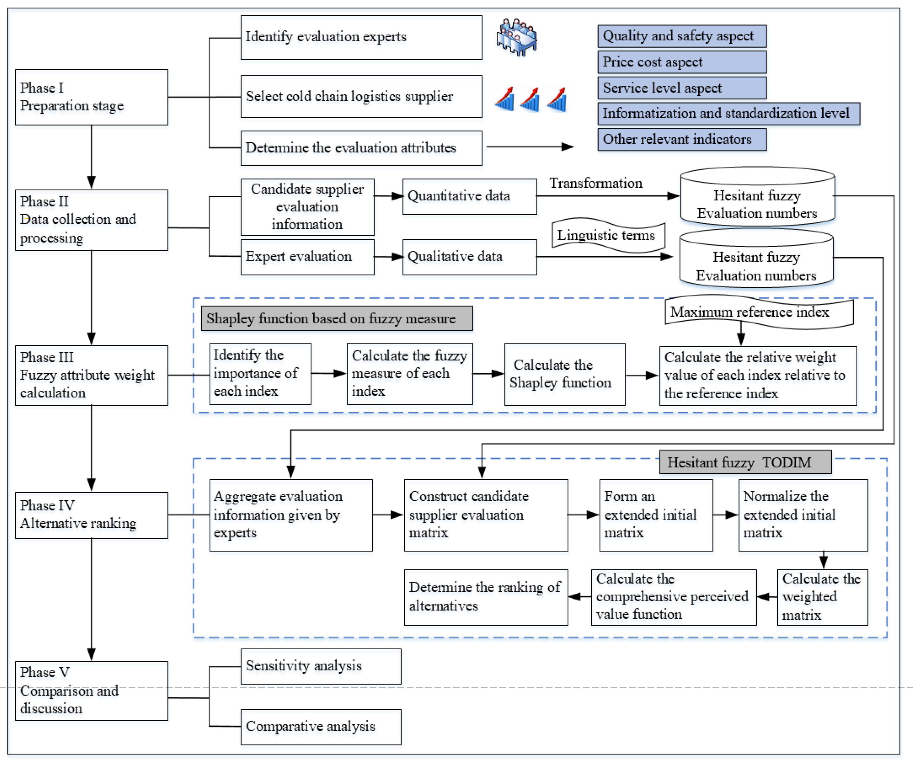
6. Case Study

6.1. A Case of Cold Chain Logistics Supplier Selection

A cold chain logistics enterprise is a livelihood guarantee for people in a city and a key supporting enterprise in the transportation industry. Since its establishment, it has always implemented and strictly implemented the business philosophy of “honest management, standardized operation; customer first, value-added service”, adhered to the management policy of “integrating safety into blood and putting customers at the top of its heart”, and won the trust of customers with high-quality, considerate, safe, and efficient cold chain logistics services, making the company enter a stage of rapid development. In order to provide consumers with fresher and more affordable raw food materials and better fresh retail services, a fresh food enterprise would like to select a cold chain logistics supplier. In the selection of candidate fresh suppliers, it is assumed that decision-makers show three psychological behavioral preferences in the face of risks: risk neutrality, risk aversion and risk preference. Three decision-makers, including a food safety engineer (E₁), a logistics management engineer (E₂), and a marketing engineer (E₃), evaluate the indicators of six candidate fresh suppliers (A₁, A₂, A₃, A₄, A₅, A₆) under the three risky conditions (good, medium, bad), wherein the probability of the future market prospect is (p₁ = 0.6, p₂ = 0.3, p₃ = 0.1). The probability of the future market prospect is also predicted by the three decision-makers.

The experts use fuzzy numbers to evaluate the five fresh suppliers under three risky conditions. In condition s₁, the evaluation information of the three decision-makers on each indicator of candidate fresh suppliers is shown in

Table 3. Hesitant Fuzzy Evaluation Information of E₁ Under Condition S₁.

	C1	C2	C4	C4	C5
A1	H{0.7,0.8,0.9}	H{0.4,0.6,0.9}	H{0.4,0.9}	H{0.3,0.5,0.8}	H{0.6,0.8}
A2	H{0.2,0.4,0.6}	H{0.1,0.3,0.5}	H{0.4,0.7,0.8}	H{0.2,0.8}	H{0.5,0.6,0.7}
A3	H{0.1,0.5,0.9}	H{0.2,0.3,0.4}	H{0.3,0.4,0.7}	H{0.4,0.6,0.7}	H{0.3,0.8,0.9}
A4	H{0.2,0.4,0.5}	H{0.3,0.5,0.7}	H{0.1,0.9}	H{0.1,0.3,0.7}	H{0.4,0.5,0.8}
A5	H{0.5,0.6,0.8}	H{0.4,0.5,0.6}	H{0.7,0.8}	H{0.2,0.3,0.6}	H{0.2,0.4,0.6}
A6	H{0.6,0.8}	H{0.5,0.8}	H{0.2,0.8,0.9}	H{0.2,0.3,0.7}	H{0.1,0.3,0.5}

,

Table 4. Hesitant Fuzzy Evaluation Information of E₂ Under Condition S₁.

	C1	C2	C4	C4	C5
A1	H{0.6, 0.9}	H{0.5,0.6,0.8}	H{0.3,0.7,0.9}	H{0.2,0.6,0.9}	H{0.7,0.8,0.9}
A2	H{0.5,0.6}	H{0.2,0.3}	H{0.5,0.6,0.8}	H{0.1,0.2,0.7}	H{0.4,0.6,0.7}
A3	H{0.3,0.4,0.8}	H{0.1,0.4}	H{0.2,0.6,0.7}	H{0.5,0.6,0.7}	H{0.5,0.6,0.7}
A4	H{0.2,0.5}	H{0.4,0.5,0.7}	H{0.4,0.5,0.9}	H{0.3,0.7}	H{0.4,0.6,0.8}
A5	H{0.5,0.6,0.7}	H{0.3,0.5,0.8}	H{0.6,0.8}	H{0.1,0.3}	H{0.3,0.4,0.6}
A6	H{0.6,0.8,0.9}	H{0.5,0.6,0.8}	H{0.1,0.8 }	H{0.3,0.6}	H{0.4,0.7}

and

Table 5. Hesitant Fuzzy Evaluation Information of E₃ Under Condition S₁.

	C1	C2	C4	C4	C5
A1	H{0.1,0.5,0.9}	H{0.3,0.9}	H{0.4,0.6,0.9}	H{0.2,0.5,0.8}	H{0.6,0.8,0.9}
A2	H{0.6,0.7}	H{0.1,0.3}	H{0.4,0.6}	H{0.2,0.5,0.6}	H{0.5,0.7}
A3	H{0.5,0.9}	H{0.1,0.4,0,7}	H{0.4,0.6,0.7}	H{0.5,0.6,0.7}	H{0.3,0.8}
A4	H{0.2,0.4,0.5}	H{0.4,0.5,0.7}	H{0.1,0.4,0.9}	H{0.3,0.6,0.7}	H{0.4,0.5,0.8}
A5	H{0.4,0.6,0.8}	H{0.4,0.5,0.6}	H{0.7,0.8}	H{0.2,0.3,0.6}	H{0.2,0.4,0.6}
A6	H{0.8,0.9}	H{0.2,0.7}	H{0.1,0.9}	H{0.2,0.6,0.7}	H{0.3,0.5}

. Among them, element H{0.7,0.8,0.9} in the table indicates that the first decision-maker holds three views on the quality safety indicator C₁ of the A₁ fresh supplier candidate, and its evaluation value maybe 0.7, 0.8 or 0.9. The other elements in the table have similar meanings.

From Table 3, Table 4 and Table 5, the numbers of elements are different. According to Definition 4, the numbers of elements are expanded to make all elements of the hesitant fuzzy evaluation value have the same number. In condition s₁, decision-makers are a type of risk aversion. Therefore, the second case in Definition 4 is used to expand the elements in the table, and the third and first cases in Definition 4 are used to expand the elements in conditions s₂ and s₃, respectively. The evaluation matrixes are normalized, and the decision matrix of the decision makers’ hesitant fuzzy standardization on the indicators of the candidate fresh suppliers is obtained under condition s₁, as shown in

Table 6. Comprehensive Evaluation Under Condition S₁.

	C1	C2	C4	C4	C5
A1	H{0.5,0.6,0.9}	H{0.4,0.5,0.9}	H{0.4,0.6,0.9}	H{0.2,0.5,0.8}	H{0.6,0.7,0.9}
A2	H{0.4,0.5,0.6}	H{0.1,0.2,0.4}	H{0.4,0.6,0.7}	H{0.2,0.3,0.7}	H{0.5,0.6,0.7}
A3	H{0.3,0.5,0.9}	H{0.1,0.3,0.5}	H{0.3,0.5,0.7}	H{0.5,0.6,0.7}	H{0.4,0.6,0.8}
A4	H{0.1,0.3,0.5}	H{0.4,0.5,0.7}	H{0.2,0.3,0.9}	H{0.2,0.4,0.7}	H{0.4,0.5,0.8}
A5	H{0.5,0.6,0.8}	H{0.4,0.5,0.7}	H{0.7,0.7,0.8}	H{0.2,0.2,0.6}	H{0.2,0.4,0.6}
A6	H{0.6,0.7,0.8}	H{0.4,0.4,0.8}	H{0.1,0.3,0.9}	H{0.2,0.4,0.7}	H{0.3,0.3,0.6}

.

The evaluation indicators of candidate fresh suppliers have mutual influences on each other, and the importance degree of each indicator is calculated. According to the importance degrees $\mu (C_1)=0.8$, $\mu (C_2)=0.4$, $\mu (C_3)=0.4$, $\mu (C_4)=0.2$, and $\mu (C_5)=0.2$ given by the experts, it can be obtained from Equation (3) that $\lambda =-0.935$. The fuzzy measures of each indicator subset are calculated according to Equation (2) and the $\lambda$ value, as shown in

Table 7. Fuzzy Measure Under Condition S₁.

Fuzzy Measure	Value	Fuzzy Measure	Value	Fuzzy Measure	Value	Fuzzy Measure	Value
$\mu (C_1)$	0.8	$\mu (C_1,C_5)$	0.552	$\mu (C_1,C_2,C_4)$	0.721	$\mu (C_3,C_4,C_5)$	0.322
$\mu (C_2)$	0.4	$\mu (C_2,C_3)$	0.331	$\mu (C_1,C_2,C_5)$	0.687	$\mu (C_1,C_2,C_3,C_4)$	0.894
$\mu (C_3)$	0.4	$\mu (C_2,C_4)$	0.461	$\mu (C_1,C_3,C_4)$	0.673	$\mu (C_1,C_3,C_4,C_5)$	0.734
$\mu (C_4)$	0.2	$\mu (C_2,C_5)$	0.319	$\mu (C_1,C_3,C_5)$	0.709	$\mu (C_1,C_2,C_3,C_5)$	0.882
$\mu (C_5)$	0.2	$\mu (C_3,C_4)$	0.345	$\mu (C_1,C_4,C_5)$	0.564	$\mu (C_1,C_2,C_4,C_5)$	0.871
$\mu (C_1,C_2)$	0.574	$\mu (C_3,C_5)$	0.376	$\mu (C_2,C_3,C_4)$	0.461	$\mu (C_2,C_3,C_4,C_5)$	0.573
$\mu (C_1,C_3)$	0.563	$\mu (C_4,C_5)$	0.176	$\mu (C_2,C_3,C_5)$	0.412	$\mu (C_1,C_2,C_3,C_4,C_5)$	1
$\mu (C_1,C_4)$	0.521	$\mu (C_1,C_2,C_3)$	0.788	$\mu (C_2,C_4,C_5)$	0.369

.

According to Equation (5) and Table 7, the Shapely weight value of each indicator is calculated as $g_1^1(g,X)={\omega }_1^1=0.36$, $g_2^1(g,X)={\omega }_2^1=0.21$, $g_3^1(g,X)={\omega }_3^1=0.24$, $g_4^1(g,X)={\omega }_4^1=0.11$, and $g_5^1(g,X)={\omega }_5^1=0.08$. The reference indicator ${\omega }_r^1={\omega }_1^1=0.36$ with the largest weight under the condition $s_1$ is obtained. According to Equation (10), the relative weight values ${\omega }_{1r}^1=1$, ${\omega }_{2r}^1=0.583$, ${\omega }_{3r}^1=0.667$, ${\omega }_{4r}^1=0.306$, and ${\omega }_{5r}^1=0.25$ of each indicator relative to the reference index are calculated.

According to Equations (9) and (10), the values of the perceived value function of each fresh candidate supplier $x_i^1$($i=1,2,\cdots ,m$) relative to the candidate $x_w^1$($w=1,2,\cdots ,m$) are calculated, where the attenuation coefficient

$\theta$ facing “loss” in Equation (10) is set as 1. The values of the relative perceived value function obtained under condition s₁ are shown in

Table 8. Values of Relative Perceived Value Function Under Condition S₁.

${\vartheta }^1(x_1,x_1)$	0	${\vartheta }^1(x_2,x_1)$	−5.44	${\vartheta }^1(x_3,x_1)$	−3.69	${\vartheta }^1(x_4,x_1)$	−5.24	${\vartheta }^1(x_5,x_1)$	−4.77	${\vartheta }^1(x_6,x_1)$	−4.74
${\vartheta }^1(x_1,x_2)$	0.93	${\vartheta }^1(x_2,x_2)$	0	${\vartheta }^1(x_3,x_2)$	−0.05	${\vartheta }^1(x_4,x_2)$	−2.54	${\vartheta }^1(x_5,x_2)$	−2.09	${\vartheta }^1(x_6,x_2)$	−2.08
${\vartheta }^1(x_1,x_3)$	−1.00	${\vartheta }^1(x_2,x_3)$	−3.90	${\vartheta }^1(x_3,x_3)$	0	${\vartheta }^1(x_4,x_3)$	−4.18	${\vartheta }^1(x_5,x_3)$	−3.07	${\vartheta }^1(x_6,x_3)$	−3.87
${\vartheta }^1(x_1,x_4)$	0.95	${\vartheta }^1(x_2,x_4)$	−1.46	${\vartheta }^1(x_3,x_4)$	−0.27	${\vartheta }^1(x_4,x_4)$	0	${\vartheta }^1(x_5,x_4)$	−2.28	${\vartheta }^1(x_6,x_4)$	−1.57
${\vartheta }^1(x_1,x_5)$	−0.29	${\vartheta }^1(x_2,x_5)$	−2.39	${\vartheta }^1(x_3,x_5)$	−2.37	${\vartheta }^1(x_4,x_5)$	−1.98	${\vartheta }^1(x_5,x_5)$	0	${\vartheta }^1(x_6,x_5)$	−1.04
${\vartheta }^1(x_1,x_6)$	0.10	${\vartheta }^1(x_2,x_6)$	−2.45	${\vartheta }^1(x_3,x_6)$	−1.31	${\vartheta }^1(x_4,x_6)$	−0.83	${\vartheta }^1(x_5,x_6)$	−1.62	${\vartheta }^1(x_6,x_6)$	0

.

The values of the comprehensive perceived value function of candidate fresh suppliers under condition s₁ are calculated. Similarly, the values of the comprehensive perceived value function under conditions s₂ and s₃ can be obtained, as shown in

Table 9. Values Of the Comprehensive Relative Perceived Value Function Under Three Conditions.

${\mathrm{\Phi }}^1(x_1)$	1	${\mathrm{\Phi }}^2(x_1)$	1	${\mathrm{\Phi }}^3(x_1)$	1
${\mathrm{\Phi }}^1(x_2)$	0	${\mathrm{\Phi }}^2(x_2)$	0	${\mathrm{\Phi }}^3(x_2)$	0
${\mathrm{\Phi }}^1(x_3)$	0.49	${\mathrm{\Phi }}^2(x_3)$	0.22	${\mathrm{\Phi }}^3(x_3)$	0.37
${\mathrm{\Phi }}^1(x_4)$	0.05	${\mathrm{\Phi }}^2(x_4)$	0.26	${\mathrm{\Phi }}^3(x_4)$	0.15
${\mathrm{\Phi }}^1(x_5)$	0.11	${\mathrm{\Phi }}^2(x_5)$	0.86	${\mathrm{\Phi }}^3(x_5)$	0.44
${\mathrm{\Phi }}^1(x_6)$	0.14	${\mathrm{\Phi }}^2(x_6)$	0.55	${\mathrm{\Phi }}^3(x_6)$	0.13

.

According to Equation (12), the values of the final comprehensive perceived value function are calculated, and the final results are $\mathrm{\Phi }(x_1)$ = 1, $\mathrm{\Phi }(x_2)$ = 0, $\mathrm{\Phi }(x_3)$ = 0.397, $\mathrm{\Phi }(x_4)$ = 0.123, $\mathrm{\Phi }(x_5)$ = 0.368, and $\mathrm{\Phi }(x_6)$ = 0.262.

Therefore, the first candidate fresh supplier is the optimal supplier.

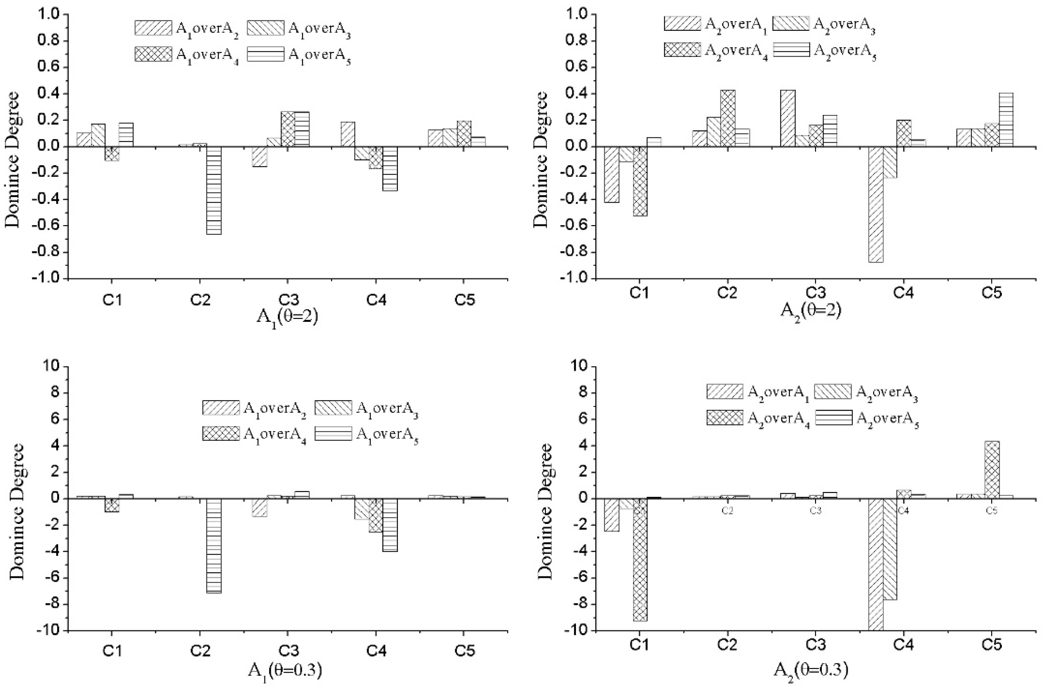
6.2. Sensitive Analysis

In the TODIM method, the change in the “loss” attenuation coefficient has a great impact on the sorting results, which is the impact of the change in the contrast value on the sorting results. Select different “loss” attenuation coefficients to calculate the comprehensive perceived value function and rank the results of each scheme, as shown in

Table 10. Ranking Table of Perceived Value Functions with Different “loss” Attenuation Coefficients.

	$\theta =0.3$		$\theta =0.6$		$\theta =1$		$\theta =1.5$		$\theta =1.9$		$\theta =2$
	Value	Sort	Value	Sort	Value	Sort	Value	Sort	Value	Sort	Value	Sort
A1	1	1	1	1	1	1	1	1	1	1	1	1
A2	0	6	0	6	0	6	0	6	0	6	0	6
A3	0.832	2	0.827	2	0.818	2	0.739	3	0.679	2	0.668	3
A4	0.136	5	0.132	5	0.119	5	0.115	5	0.102	5	0.092	5
A5	0.528	3	0.548	3	0.577	3	0.632	2	0.673	3	0.682	2
A6	0.279	4	0.261	4	0.254	4	0.244	4	0.24	4	0.224	4
	$\theta =2.5$		$\theta =3$		$\theta =3.5$		$\theta =4$		$\theta =5.5$		$\theta =6$
	Value	Sort	Value	Sort	Value	Sort	Value	Sort	Value	Sort	Value	Sort
A1	1	1	1	1	1	1	1	1	1	1	1	1
A2	0	6	0	6	0	6	0	6	0	6	0	6
A3	0.663	3	0.658	3	0.655	3	0.651	3	0.646	3	0.643	3
A4	0.09	5	0.088	5	0.0.85	5	0.083	5	0.081	5	0.079	5
A5	0.699	2	0.707	2	0.714	2	0.723	2	0.731	2	0.738	2
A6	0.279	4	0.254	4	0.24	4	0.196	4	0.194	4	0.192	4
	$\theta =6.5$		$\theta =7$		$\theta =7.5$		$\theta =7.5$		$\theta =8$		$\theta =8.3$
	Value	Sort	Value	Sort	Value	Sort	Value	Sort	Value	Sort	Value	Sort
A1	1	1	1	1	1	1	1	1	1	1	1	1
A2	0	6	0	6	0	6	0	6	0	6	0	6
A3	0.638	2	0.625	2	0.612	2	0.605	3	0.587	3	0.581	3
A4	0.078	5	0.076	5	0.075	5	0.074	5	0.073	5	0.072	5
A5	0.743	3	0.751	3	0.758	3	0.765	2	0.779	2	0.786	2
A6	0.19	4	0.188	4	0.187	4	0.185	4	0.183	4	0.18	4
	$\theta =8.6$		$\theta =9$		$\theta =9.3$		$\theta =9.5$		$\theta =9.9$		$\theta =10$
	Value	Sort	Value	Sort	Value	Sort	Value	Sort	Value	Sort	Value	Sort
A1	1	1	1	1	1	1	1	1	1	1	1	1
A2	0	6	0	6	0	6	0	6	0	6	0	6
A3	0.575	2	0.564	2	0.553	2	0.546	3	0.533	3	0.532	3
A4	0.071	5	0.071	5	0.07	5	0.07	5	0.069	5	0.069	5
A5	0.792	3	0.798	3	0.806	3	0.814	2	0.825	2	0.827	2
A6	0.177	4	0.175	4	0.173	4	0.171	4	0.17	4	0.169	4

.

Through the comparison and analysis, we can find that as the value of $\theta$ increases, there are the following results: when $\theta \le 1.9$, $A_3$ is better than $A_5$, and when $\theta \ge 2$, $A_5$ is better than $A_3$. This is because $A_3$ has significant losses in $C_1$ and $C_4$. The gain from $C_2$, $C_3$ and $C_5$ is not obvious. However, $A_5$ has insignificant losses in $C_1$ and $C_4$. Then, when $\theta \ge 2$, $A_5$ in the final comprehensive perceived value function is greater than $A_3$. When $\theta =2$ and $\theta =0.3$, the advantages of the alternatives $A_5$ and $A_3$ over other alternatives are calculated, respectively. The results are shown in Figure 3. Through the comparison, it can be found that when $\theta =0.3$, the loss of $A_5$ and $A_3$ is amplified. It is obvious that the losses of $A_5$ are significantly greater than $A_3$. When $\theta =2$, the losses of $A_5$ are weakened in $C_1$ and $C_4$. The gains of $A_5$ are greater than $A_5$ in $C_2$, $C_3$, and $C_5$. The increased gains of $A_5$ are enough to make $A_5$ superior to $A_3$. The change in $\theta$ can effectively reflect the risk attitude of decision-makers, thus affecting the evaluation results.

6.3. Comparative Analysis

In order to verify the effectiveness of the method, different approaches are adopted to evaluate the candidate suppliers. The approaches include the method presented in this paper (HFS-TODIM), the hesitant fuzzy TODIM method without the generalized Shapley function (HF-TODIM), the method that only considers one calculation prospect situation (OPS-TODIM), the hesitant fuzzy VIKOR (HF-VIKOR) method, the hesitant fuzzy TOPSIS (HF-TOPSIS) method, the hesitant fuzzy simple additive weighting (HF-SAW) method, and the hesitant fuzzy MARCOS (HF-MARCOS) method. The comparison of the results is shown in

Table 11. Sort Results with Different Methods.

	Evaluation Results						Sort Results
HFS-TODIM	$\mathrm{\Phi }{(A)}_1$ 1	$\mathrm{\Phi }{(A)}_2$ 0	$\mathrm{\Phi }{(A)}_3$ 0.397	$\mathrm{\Phi }{(A)}_4$ 0.123	$\mathrm{\Phi }{(A)}_5$ 0.368	$\mathrm{\Phi }{(A)}_6$ 0.262	$A_1\succ A_3\succ A_5\succ A_6\succ A_4\succ A_2$
HF-TODIM	${\mathrm{\Phi }}^{\prime }{(A)}_1$ 1	${\mathrm{\Phi }}^{\prime }{(A)}_2$ 0.012	${\mathrm{\Phi }}^{\prime }{(A)}_3$ 0.673	${\mathrm{\Phi }}^{\prime }{(A)}_4$ 0	${\mathrm{\Phi }}^{\prime }{(A)}_5$ 0.492	${\mathrm{\Phi }}^{\prime }{(A)}_6$ 0.217	$A_1\succ A_3\succ A_5\succ A_6\succ A_2\succ A_4$
OPS-TODIM	${\mathrm{\Phi }}^{″}{(A)}_1$ 1	${\mathrm{\Phi }}^{″}{(A)}_2$ 0	${\mathrm{\Phi }}^{″}{(A)}_3$ 0.585	${\mathrm{\Phi }}^{″}{(A)}_4$ 0.231	${\mathrm{\Phi }}^{″}{(A)}_5$ 0.234	${\mathrm{\Phi }}^{″}{(A)}_6$ 0.462	$A_1\succ A_3\succ A_6\succ A_5\succ A_4\succ A_2$
FH-VIKOR	Q(A1) 0	Q(A2) 0.964	Q(A3) 0.354	Q(A4) 0.913	Q(A5) 0.651	Q(A6) 0.883	$A_1\succ A_3\succ A_6\succ A_5\succ A_4\succ A_2$
FH-TOPSIS	C(A1) 0.942	C(A2) 0.33	C(A3) 0.698	C(A4) 0.303	C(A5) 0.347	C(A6) 0.475	$A_1\succ A_3\succ A_6\succ A_5\succ A_2\succ A_4$
FH-SAW	S(A1) 0.868	S(A2) 0.298	S(A3) 0.772	S(A4) 0.411	S(A5) 0.53	S(A6) 0.372	$A_1\succ A_3\succ A_5\succ A_4\succ A_6\succ A_2$

.

The method of HF-TODIM is adopted to sort the fresh candidate suppliers, compared with the method in this paper, the A₁ is always the optimal supplier, but the positions of the second candidate fresh supplier and the fourth candidate fresh supplier are exchanged. The reason for the inconsistent ranking results is that although the indicator price cost (C₂) of the second candidate fresh supplier is low, the quality safety (C₁) of the products it provides is relatively poor, and the service level (C₃) is also very average. In this paper, after considering the mutual influence among the indicators, the calculation results show that the second fresh supplier ranks last. After considering the mutual influence among the indicators, the supplier selection results are more accurate and objective.

When only one prospective situation is considered (OPS-TODIM), through the results of comparative analysis, it can be seen that the first candidate fresh supplier is the optimal supplier, but the ranking sequence of the fifth candidate fresh supplier and the sixth candidate fresh supplier has been exchanged. This is because when considering the decision-maker’s risky psychological preference behavior, the ability of the fifth candidate fresh supplier to deal with risks is better than the sixth candidate fresh supplier. The risk-type supplier selection method can effectively analyze the risk-based psychological preference behavior of decision-makers.

We can find that the best performer and the worst performer obtained by the FH-VIKOR method are the same as HFS-TODIM. However, different from the HFS-TODIM method, when the FH-TOPSIS method is used, the worst performer changes from A₂ to A₄. Moreover, the positions of A₅ and A₆ are exchanged. This can be interpreted as follows. On one hand, when the FH-TOPSIS method is used for ranking, the psychological behavior of decision-makers under different market prospects is not considered. On the other hand, the IT2F-TOPSIS method only considers the distance between the evaluation value and the ideal solution and ignores its relative importance. For $A_2$ and $A_4$, $D_2^{+}=0.173$, $D_4^{+}=0.166$, $D_2^{-}=0.123$, and $D_4^{-}=0.123$. The distance between supplier $A_4$ and the ideal point is smaller than $A_2$, resulting in $A_4\succ A_2$. The sorting results obtained by the HF-SAW method are identical to the ranking order, which is obtained by the HFS-TODIM method. The effectiveness and feasibility of the HFS-TODIM method can be verified.

7. Conclusions

7.1. Managerial Implications

The relationship between enterprises and suppliers has become a long-term partnership characterized by risk sharing, information, and benefit sharing, rather than being a buying and selling relationship. Through an example analysis, the following suggestions can be given:

• By comparing the weights of various indicators, it can be found that product quality and cost are important factors in selecting suppliers. In the long run, the enterprise should maintain a good cooperative relationship with suppliers so as to ensure that the purchase price is relatively low. A revenue sharing contract can be signed with suppliers, which can ensure that the procurement cost is not too high and that the quality of products can be guaranteed.
• The different freshness of products affects the changes in the profits. Suppliers should make full use of their mature cold chain distribution system and cold storage to ensure the freshness of products and start a quality war.
• Suppliers are classified according to the sorting results, taking corresponding supplier development strategies according to the different results of supplier classification. The construction of the supplier evaluation system should be strengthened, for instance, by conducting a supplier performance evaluation. The evaluation cycle should adopt a combination of regular and irregular spot checks, and different incentives can be implemented for different suppliers.

7.2. Research Summary

With the in-depth development of the logistics industry and the continuous improvement of people’s living standards, high value-added cold chain logistics play an increasingly important role in the circulation field. Supplier selection is an important part of the procurement process of downstream enterprises (customers) in cold chain logistics. Whether we can select them comprehensively and establish a stable alliance partnership with them is related to the procurement utility of downstream enterprises (customers) and the operation efficiency of cold chain logistics.

The traditional supplier selection method does not consider the market risk factors and the risk attitude of decision-makers. The selection of suppliers is affected by the market prospects, and it is reasonable for decision-makers to adopt a risk attitude. Considering the risk attitude of the decision-makers and their hesitation in the evaluation of indicators, this paper puts to use a multi-attribute risky supplier selection method based on the hesitant fuzzy method. The main characteristics of this paper are as follows:

• The evaluation index system of cold chain logistics suppliers is determined. Based on the characteristics of cold chain logistics suppliers, we conducted comprehensive literature research and screening to determine the evaluation index. Five first-class indicators are determined, including quality and safety, price cost, service level, informatization and standardization level, and other relevant indicators. A total of 27 second-class indicators are set to build the evaluation index system of cold chain logistics suppliers. The evaluation index system can provide a certain reference value for cold chain logistics enterprises when selecting suppliers.
• Considering the risky psychological preference behavior of decision-makers, the HFS-TODIM method is used to sort the candidate suppliers by analyzing decision-maker’s risk attitudes.
• Considering the mutually influential relationship among indicators, the generalized Shapley function is used to analyze the importance degree of indicators. Next, the index weight is obtained, which is more in line with the reality.
• In light of the fuzzy characteristics of the evaluation information, hesitant fuzzy information is used to express the evaluation information of decision-makers. The decision-makers are allowed to give several possible values, which can increase the flexibility of the decision-maker’s assignment and can more delicately describe the uncertainty of things, which is especially suitable for describing the real decision-making problem in the case of hesitation.

The results show that enterprises will comprehensively consider the quality, cost, freshness, and other factors. The product competitiveness, operation, and service level of suppliers are still in a relatively important position. This method solves the subjectivity of the previous evaluation results, simplifies the complexity of the evaluation operation, and makes the evaluation results have certain reference and comparability.

7.3. The Limitations and Research Prospects

The method has been applied to the selection of candidate fresh suppliers. This example is given to verify the effectiveness of the method in this paper. At the same time, the method considers the uncertainty of the decision-making process and the relationship among the evaluation indicators, which effectively improves the accuracy of supplier selection. Combined with the characteristics of the cold chain logistics industry, aiming at the supplier evaluation index system and supplier selection, this paper provides a good theoretical basis and improvement strategy for cold chain enterprises to select suppliers, but there are still deficiencies which need to be further improved in the following two aspects:

• Enterprises usually have more than one supplier. Enterprises will divide suppliers into several groups according to the number of materials purchased, the importance of materials purchased, and the importance and reliability of suppliers to the enterprise. We only sort the suppliers and do not classify them.
• The selection of indicators has certain limitations. For example, there are many indicators of freshness, such as taste, color, and appearance. This paper integrates these small indicators, and how to judge the freshness quantitatively and qualitatively is not described in detail.

In the future, we will conduct in-depth research on cold chain logistics supplier management from the following aspects:

• With the rapid development of the cold chain logistics industry and the improvement of service quality awareness in the future, the influencing factors of cold chain logistics will be more complex, and the evaluation system will focus on a sub field of the cold chain, so the evaluation results will be more accurate.
• Any method has its advantages and disadvantages. This paper only conducts a preliminary research and exploration on the related problems of supplier evaluation based on the HFS-TODIM method. In the future, we can try to use more methods, such as the related algorithms based on artificial intelligence, to study the cold chain suppliers and apply them to practical work.

References

- Song, W.; Ming, X.; Xu, Z. Risk evaluation of customer integration in new product development under uncertainty. Comput. Ind. Eng. 2013, 65, 402–412. [Google Scholar]
- Li, D. TOPSIS-based nonlinear-programming methodology for multiattribute decision making with interval-valued intuitionistic fuzzy sets. IEEE Trans. Fuzzy Syst. 2018, 18, 299–311. [Google Scholar]
- Liao, H.; Xu, Z.; Zeng, X. Hesitant fuzzy linguistic VIKOR method and its application in qualitative multiple criteria decision making. IEEE Trans. Fuzzy Syst. 2015, 23, 1343–1355. [Google Scholar]
- Wang, P.; Zhu, Z.; Wang, Y. A novel hybrid MCDM model combining the SAW, TOPSIS and GRA methods based on experimental design. Inf. Sci. 2016, 345, 27–45. [Google Scholar]
- Wang, J.Q.; Wu, J.T.; Wang, J.; Zhang, H.Y.; Chen, X.H. Multi-criteria decision-making methods based on the Hausdorff distance of hesitant fuzzy linguistic numbers. Soft Comput. 2016, 20, 1621–1633. [Google Scholar]
- Wan, S.; Xu, G.; Dong, J. Supplier selection using ANP and ELECTRE II in interval 2-tuple linguistic environment. Inf. Sci. 2017, 385–386, 19–38. [Google Scholar]
- Kahneman, D.; Tversky, A. Prospect theory: An analysis of decision under risk. Econometrica 1979, 47, 263–291. [Google Scholar]
- Tversky, A.; Kahneman, D. Advances in prospect theory: Cumulative representation of uncertainty. J. Risk Uncertain. 1992, 5, 297–323. [Google Scholar]
- Dai, W.F.; Zhong, Q.Y.; Qi, C.Z. Multi-stage multi-attribute decision-making method based on the prospect theory and triangular fuzzy MULTIMOORA. Soft Comput. 2018, 24, 9429–9440. [Google Scholar]
- Li, Y.L.; Ying, C.S.; Chin, K.S.; Yang, H.T.; Xu, J. Third-party Reverse Logistics Provider Selection Approach Based on Hybrid-Information MCDM and Cumulative Prospect Theory. J. Clean. Prod. 2018, 195, 573–584. [Google Scholar]
- Gomes, L.F.; Lima, M.M. TODIM: Basic and application to multicriteria ranking of projects with environment impacts. Found. Comput. Decis. Sci. 1991, 16, 113–127. [Google Scholar]
- Tian, X.; Niu, M.; Ma, J.; Xu, Z. A novel TODIM with probabilistic hesitant fuzzy information and its application in green supplier selection. Complexity 2020, 2020, 2540798. [Google Scholar]
- Liu, L.; Song, W.; Han, W. How sustainable is smart PSS? An integrated evaluation approach based on rough BWM and TODIM. Adv. Eng. Inform. 2020, 43, 101042. [Google Scholar]
- Li, M.Y.; Cao, P.P. Extended TODIM method for multi-attribute risk decision making problems in emergency response. Comput. Ind. Eng. 2018, 135, 1286–1293. [Google Scholar]
- Qin, Q.; Liang, F.; Li, L.; Chen, Y.; Yu, G. A TODIM-based multi-criteria group decision making with triangular intuitionistic fuzzy numbers. Appl. Soft Comput. 2017, 55, 93–107. [Google Scholar]
- Ren, H.; Liu, M.; Zhou, H. Extended TODIM Method for MADM Problem under Trapezoidal Intuitionistic Fuzzy Environment. Int. J. Comput. Commun. Control. (IJCCC) 2019, 14, 220–232. [Google Scholar]
- Zhang, G.; Wang, J.Q.; Wang, T.L. Multi-criteria group decision-making method based on TODIM with probabilistic interval-valued hesitant fuzzy information. Expert Syst. 2019, 36, e12424. [Google Scholar]
- Liu, D.; Liu, Y.; Wang, L. Distance measure for Fermatean fuzzy linguistic term sets based on linguistic scale function: An illustration of the TODIM and TOPSIS methods. Int. J. Intell. Syst. 2019, 34, 2807–2834. [Google Scholar]
- Liu, H.; Rodríguez, R.M. A fuzzy envelope for hesitant fuzzy linguistic term set and its application to multicriteria decision making. Inf. Sci. 2014, 258, 220–238. [Google Scholar]
- Shi, M.H.; Xiao, Q.X. Hesitant fuzzy linguistic aggregation operators based on global vision. J. Intell. Fuzzy Syst. 2017, 33, 193–206. [Google Scholar]
- Fahmi, A.; Abdullah, S.; Amin, F.; Asad, A.; Ahmad, K. Some geometric operators with triangular cubic linguistic hesitant fuzzy number and their application in group decision-making. J. Intell. Fuzzy Syst. 2018, 35, 2485–2499. [Google Scholar]
- Grabisch, M.; Labreuce, C. A decade of application of the Choquet and sugeno integrals in multi-criteria decision aid. Ann. Oper. Res. 2008, 6, 1–44. [Google Scholar]
- Shao, S.; Zhang, X.; Zhao, Q. Multi-Attribute Decision Making Based on Probabilistic Neutrosophic Hesitant Fuzzy Choquet Aggregation Operators. Symmetry 2019, 11, 623. [Google Scholar]
- Peng, X.D.; Yang, Y. Pythagorean Fuzzy Choquet Integral Based MABAC Method for Multiple Attribute Group Decision Making. Int. J. Intell. Syst. 2016, 31, 989–1020. [Google Scholar]
- Weng, X.; An, J.; Hui, Y. The Analysis of the Development Situation and Trend of the City-Oriented Cold Chain Logistics System for Fresh Agricultural Products. Open J. Soc. Sci. 2015, 3, 70–80. [Google Scholar]
- Li, G. Development of cold chain logistics transportation system based on 5G network and Internet of things system. Microprocess. Microsyst. 2020, 80, 103565. [Google Scholar]
- Xiong, Y.; Zhao, J.; Lan, J. Performance Evaluation of Food Cold Chain Logistics Enterprise Based on the AHP and Entropy. Int. J. Inf. Syst. Supply Chain. Manag. 2019, 12, 57–67. [Google Scholar]
- Lau, H.; Nakandala, D.; Shum, P.K. A business process decision model for fresh-food supplier evaluation. Bus. Process Manag. J. 2018, 24, 716–744. [Google Scholar]
- Pang, J.; Liang, J.; Song, P. An adaptive consensus method for multi-attribute group decision making under uncertain linguistic environment. Appl. Soft Comput. 2017, 58, 339–353. [Google Scholar]
- Bian, T.; Hu, J.; Deng, Y. Identifying influential nodes in complex networks based on AHP. Phys. A Stat. Mech. Its Appl. 2017, 479, 422–436. [Google Scholar]
- Türk, A.; Zkk, M. Shipyard location selection based on fuzzy AHP and TOPSIS. J. Intell. Fuzzy Syst. 2020, 39, 4557–4576. [Google Scholar]
- Mohamed, A.B.; Mai, M.; Florentin, S. A Hybrid Neutrosophic Group ANP-TOPSIS Framework for Supplier Selection Problems. Symmetry 2018, 10, 200–226. [Google Scholar]
- Liang, D.C.; Xu, Z.S.; Liu, D.; Wu, Y. Method for three-way decisions using ideal TOPSIS solutions at Pythagorean fuzzy information. Inf. Sci. Int. J. 2018, 435, 282–295. [Google Scholar]
- Hu, Y.J.; Wu, L.Z.; Shi, C.; Wang, Y.L.; Zhu, F.F. Research on optimal decision-making of cloud manufacturing service provider based on grey correlation analysis and TOPSIS. Int. J. Prod. Res. 2020, 58, 748–757. [Google Scholar]
- Awasthi, A.; Kannan, B.K. Green supplier development program selection using NGT and VIKOR under fuzzy environment. Comput. Ind. Eng. 2016, 91, 100–108. [Google Scholar]
- Sari, K. A novel multi-criteria decision framework for evaluating green supply chain management practices. Comput. Ind. Eng. 2017, 105, 338–347. [Google Scholar]
- Saati, S.; Hatami-Marbini, A.; Agrell, P.J.; Tavana, M. A common set of weight approach using an ideal decision-making unit in data envelopment analysis. J. Ind. Manag. Optim. 2013, 8, 623–637. [Google Scholar]
- Puri, J.; Yadav, S. A concept of fuzzy input mix-efficiency in fuzzy DEA and its application in banking sector. Expert Syst. Appl. 2013, 40, 1437–1450. [Google Scholar]
- Chen, T. An ELECTRE-based outranking method for multiple criteria group decision making using interval type-2 fuzzy sets. Inf. Sci. 2014, 263, 1–21. [Google Scholar]
- Das, S.; Guha, D.; Mesiar, R. Extended Bonferroni Mean Under Intuitionistic Fuzzy Environment Based on a Strict t-Conorm. IEEE Trans. Syst. Man Cybern. Syst. 2017, 47, 2083–2099. [Google Scholar]
- Wang, J.Q.; Peng, L.; Zhang, H.Y.; Xiao, X.H. Method of multi-criteria group decision-making based on cloud aggregation operators with linguistic information. Inf. Sci. 2014, 274, 177–191. [Google Scholar]
- Mou, Q.; Xu, Z.; Liao, H. An intuitionistic fuzzy multiplicative best_worst method for multi-criteria group decision making. Inf. Sci. 2016, 374, 224–239. [Google Scholar]
- Wu, Y.; Wu, C.; Zhou, J.; Zhang, B.; Xu, C.; Yan, Y.; Liu, F. A DEMATEL-TODIM based decision framework for PV power generation project in expressway service area under an intuitionistic fuzzy environment—ScienceDirect. J. Clean. Prod. 2020, 247, 119099. [Google Scholar]
- Hedi, E.; Ganouati, J.; Stephane, V. A mean-maverick game cross-efficiency approach to portfolio selection: An application to Paris stock exchange. Expert Syst. Appl. 2018, 113, 161–185. [Google Scholar]
- Liu, X.; Wan, S. A method to calculate the ranges of criteria weights in ELECTRE I and II methods. Comput. Ind. Eng. 2019, 137, 106067. [Google Scholar]
- Chen, H.; Li, J. How to build a fresh food cold chain logistics service quality evaluation index system. Mech. Eng. 2013. [Google Scholar] [CrossRef]
- Zhang, H.; Shi, Y.; Qiu, B. Applying catastrophe progression method to evaluate the service quality of cold chain logistics. Complex Intell. Syst. 2020, 1–15. [Google Scholar] [CrossRef]
- Zhu, L. Economic Analysis of a Traceability System for a Two-Level Perishable Food Supply Chain. Sustainability 2017, 9, 682. [Google Scholar]
- Aworh, O. Food safety issues in fresh produce supply chain with particular reference to sub-Saharan Africa. Food Control 2020, 123, 107737. [Google Scholar]
- Saen, R.F.; Wang, J. Suppliers Selection in Volume Discount Environments in the Presence of Both Cardinal and Ordinal Data. Int. J. Inf. Syst. Supply Chain. Manag. 2011, 2, 69–81. [Google Scholar]
- Zhao, H.; Guo, S. Selecting Green Supplier of Thermal Power Equipment by Using a Hybrid MCDM Method for Sustainability. Sustainability 2014, 6, 217–235. [Google Scholar]
- Nguyen, N.; Lin, G.H.; Dang, T.T. A Two Phase Integrated Fuzzy Decision-Making Framework for Green Supplier Selection in the Coffee Bean Supply Chain. Mathematics 2021, 9, 1923. [Google Scholar]
- Liu, H.; Nie, S. Low Carbon Scheduling Optimization of Flexible Integrated Energy System Considering CVaR and Energy Efficiency. Sustainability 2019, 11, 5375. [Google Scholar]
- Wan, S.-P.; Zou, W.-C.; Zhong, L.-G.; Dong, J.-Y. Some new information measures for hesitant fuzzy PROMETHEE method and application to green supplier selection. Soft Comput. 2019, 24, 9179–9203. [Google Scholar]
- Yang, L.; Tan, T.; Wu, Z.; Zheng, S.; Cheng, J. A Primary Analysis on the Food Recall System: A Hard Mountain for China to Climb. Int. J. Soc. Sci. Stud. 2015, 3, 50–55. [Google Scholar]
- Azadeh, A.; Keramati, A.; Karimi, A.; Sharahi, Z.J.; Pourhaji, P. Design of integrated information system and supply chain for selection of new facility and suppliers by a unique hybrid meta-heuristic computer simulation algorithm. Int. J. Adv. Manuf. Technol. 2014, 71, 775–793. [Google Scholar]
- Li, J.; Zheng, S.; Ying, T. The Effect of Information Utilization: Introducing a Novel Guiding Spark in the Fireworks Algorithm. IEEE Trans. Evol. Comput. 2017, 21, 153–166. [Google Scholar]
- Rezaei, A.; Aghsami, A.; Rabbani, M. Supplier selection and order allocation model with disruption and environmental risks in centralized supply chain. Int. J. Syst. Assur. Eng. Manag. 2021, 12, 1036–1072. [Google Scholar]
- Xu, Z. Choquet integrals of weighted intuitionistic fuzzy information. Inf. Sci. 2010, 180, 726–736. [Google Scholar]
- Tan, C.; Jiang, Z.Z.; Chen, X. An extended TODIM method for hesitant fuzzy interactive multicriteria decision making based on generalized Choquet integral. Journal of intelligent & fuzzy systems. Appl. Eng. Technol. 2015, 29, 293–305. [Google Scholar]