Article

A Novel Sustainable Processing Mode for Burr Classified Prediction of Weak Rigid Drilling Process Using a Fusion Modeling Method

Institute of Artificial Intelligence, Donghua University, Shanghai 201600, China
*
Author to whom correspondence should be addressed.
Sustainability 2022, 14(12), 7429; https://doi.org/10.3390/su14127429
Submission received: 4 May 2022 / Revised: 7 June 2022 / Accepted: 15 June 2022 / Published: 17 June 2022

Abstract

:
Weakly rigid drilling systems, such as the industrial robot, are widely used in aerospace, military, and other fields due to its good flexibility and large scope of operation. However, the weak rigidity can easily cause burrs, seriously affecting the precision of parts and product performance. To reduce the heavy deburring process and to improve continuous production and sustainable processing capacity, accurate prediction of burr quality is a prerequisite. Traditional burr forming theory cannot accurately predict the drilling defects. Data-driven approaches can be independent of prior knowledge and discover relationships between process parameters and machining precision directly from the data structure itself. Therefore, to take advantage of both approaches, a fusion model was established for burr classified prediction. On the one hand, the drilling and burr forming process was firstly modeled, and preliminary classification results for burrs were calculated. On the other hand, according to the measured data, the errors between initial calculation results and actual classification results were obtained and selected as the tag values of dataset, which served as inputs for the error compensation model of burrs. Finally, by training the network of TCN–DNN using the drilling data, the burr classified prediction in a weak rigid hole-making system was realized. Experimental results showed that compared with traditional drilling theory, the prediction accuracy of the proposed model improved by 25%, reaching 91.67%. The results can provide a basis for judging the process of burr post-treatment, which has practical guiding significance. This method is beneficial to reduce the heavy deburring process and to improve sustainable processing capacity.

1. Introduction

Automatic hole-making by industrial robots is widely used in aerospace, military, and other fields [1,2]. As its system stiffness is usually less than 1/10 of traditional CNC machine tools, there will be strong vibration under the action of large drilling force, and as such it is difficult to guarantee processing quality. This will lead to unpredictable burr quality and heavy deburring processes in late processing. To improve continuous production and sustainable manufacturing capacity, accurate prediction of burr quality is a prerequisite. By accurately implementing burr classified prediction in weak rigid hole-making systems, substandard products can be targeted, and reprocessing and process parameters can be effectively optimized, which can significantly improve the quality and efficiency.
Generally, machining systems with rigidity lower than 7 × 10⁶ N/m are defined as weak rigid systems [3,4]. Taking the drilling technology of anti-aircraft tanks as an example, the bolt mounting holes on the car frame have the characteristics of scattered positions and large-span hole pitches. It is difficult to control burrs when using industrial robots to make holes because of insufficient rigidities of the system. In the actual hole-making process, as the drilling force changes, the machining tremor of the weak rigid system increases, working time becomes longer, surface integrity of the holes becomes worse, and burrs become larger. It is easy to cause fatigue failure of mounting holes and serious safety accidents [5,6].
Due to the weak rigidity of the system, the drilling process will bring about considerable instability and uncertainty. Traditional burr forming theory cannot accurately predict the drilling deflections. In the working process of the weak rigid hole-making system, there are two main types of factors affecting the drilling performance: the geometric factors involving the diameter-to-length (D:L) ratio, hole tolerance, center-drill, surface preparation, plate structure, etc.; and the dynamic factors involving the drilling force, drilling temperature, tooling equipment, the spindle speed, feed, etc. Furthermore, there is a coupling relationship among these factors. Thus, it is almost impossible to build an analytical model that can accurately predict the burrs. A data-driven approach can be independent of prior knowledge and discover relationships between process parameters and machining precision directly from the data structure itself. However, the pure data-driven model is overly context-dependent and inadaptable to complex forecasting problems, and it is difficult to maintain high accuracy.
In this paper, mechanical characteristics of the drilling process in weak rigid systems will be firstly studied, and then the data-driven approach will be deeply integrated to construct a novel burr-classified prediction model. This fusion model uses the mechanism model to guide the data-driven model and performs multi-stage compensation correction to improve the prediction performance.

2. Literature Review

The current research mainly focuses on burr control of drilling systems from three perspectives: (1) Optimized machining parameters. Zai et al. [7] took full account of the power capability of the hole-drilling system, involving axial force power, material deformation power, and the total power, and calculated the burr height according to the energy conservation method. Zheng [8] optimized parameter combinations by constructing a satisfaction function. Mondal et al. [9] established a second-order regression model of burr height and used a flower pollination algorithm to select the optimal process parameters. (2) Optimized processing equipment. Jia et al. [10] proposed a new step drill structure to reduce delamination and burrs by controlling the step diameter ratio. Kwon et al. [11] developed a step drill that could minimize delamination and uncut fibers while processing carbon fiber-reinforced plastics (CFRP), optimizing drilling quality. (3) Using auxiliary machining technology. Hassan et al. [12] developed a new analytical model to describe the formation of inlet burrs as a function of tool geometry, operating parameters, and workpiece material properties during machining ductile metals. Hu et al. [13] studied robot rotary ultrasonic drilling under a weak rigid environment and verified the influence of high-frequency vibration on burr height. Li et al. [14] studied the influence of vibration-assisted drilling on outlet burrs and concluded that vibration amplitude was the most sensitive to burrs. Yang et al. [15] investigated an error compensation strategy that could simultaneously consider the datum error, fixture error, tool path error, and workpiece deformation error, effectively solving the error synthesis problem when using auxiliary machining equipment. It is observed that at present, the mechanism of flutter and burr forming in weak rigid hole-making systems is not clear. Therefore, an important means to improve the machining accuracy and drilling quality of automatic hole-making system is by studying the burr formation rule in weak rigid system and establishing the burr prediction model.
The data-driven method is a research hotspot in industry, which can explore the relationship between data structures directly from the data itself without relying on prior knowledge. Chen et al. [16] introduced machine vibration signals and operation information based on the logistic regression neural network model and effectively evaluated the reliability of CNC machine tools. Gebraeel and Lawley [17] introduced a neural network into the research of bearing life prediction and accurately predicted the residual life distribution of the bearing with its vibration signal as the model input. Yang et al. [18] established and compared a variety of milling force models using a lot of experimental data, and on that basis, Chang et al. [19] modeled drilling forces in the deep hole drilling scenario with single boring and trepanning associations and derived critical conditions for drilling vibrations with a steady state. Zheng et al. [20] established a stress calculation model of the tool edge for micro-drilling and studied a neural network model in terms of tool wear state based on vibration signals. Rimpault et al. [21] studied the burr height prediction model of a hybrid laminated composite with CFRP, titanium alloy, and aluminum alloy using data-driven analysis methods. An et al. [22] addressed sequence data in the task of tool remaining useful life prediction by incorporating a convolutional neural network with a stacked bi-directional and uni-directional LSTM network. Moreover, they proposed a novel integrated model based on deep learning and multi-sensor feature fusion, successfully realizing cutting tool monitoring and bearing fault diagnosis [23]. However, the data-driven approach is overly context-dependent and inadaptable to complex forecasting problems, which makes it difficult to maintain high accuracy. How to use the mechanism model to guide the data-driven model for performing multi-stage compensation correction so as to improve the prediction performance [24,25] is becoming a new development direction for the fusion of mechanism and data.
In recent years, scholars have tried the fusion modeling method of mechanism and data, which provides a new idea for burr classified prediction. Abd-Elwahed [26] utilized response surface analysis and artificial neural networks to model and evaluate the effect of control parameters, effectively increasing the prediction accuracy. Gaitonde and Karnik [27] developed burr size models required for PSO optimization using an artificial neural network with the drilling experiments planned as per full factorial design. Gan et al. [28] proposed a hierarchical diagnosis network by collecting deep belief networks for the hierarchical identification of a mechanical system. Wang et al. [29] established a data-driven model of fault diagnosis for rotating machinery and proposed a model updating a scheme based on parameter sensitivity analysis. Yu et al. [30] proposed a data framework using non-parametric Bayesian networks and reduced the error caused by unknown mechanism structures of complex systems. For unknown exceptions that may occur during status detection, Booyse et al. [31] proposed a deep data fusion framework that could monitor the entity model state without relying on historical failure data. Luo et al. [32] proposed a reliability maintenance method for NC machine tools based on the fusion of the mechanism model and the data-driven model, which combined the theoretical model and particle swarm optimization algorithm effectively, significantly improving the reliability of the fusion model. Wang et al. [33] integrated nonlinear and linear dynamic decoupling models into the data model, which increased the prediction efficiency and data model precision. Hu et al. [34] proposed a construction method for a high fidelity model, which described and defined models from three levels, including geometry, mechanism, and data, to achieve knowledge acquisition and data mapping. Although mechanism and data fusion modeling are developing continuously, there is still room for research on fusion modeling methods of machining processes [35,36]. At present, the application of burr prediction and control is still seriously lacking. Traditional burr prediction is based on the prior estimation of machining parameters, which cannot monitor the workpiece state in real time. In the working process of the weak rigid hole-making system, the dynamic parameters such as stiffness are changing continuously, tools wear quickly, and drilling loads change constantly. The information related to burr generation not only includes the spindle speed, feed, tool parameters, and robot pose, but also includes power, current, drilling force, etc., and there is a coupling relationship among these factors. Thus, it is almost impossible to build an analytical model that can accurately predict the burrs. Therefore, it is necessary to put forward a method of mass data acquisition and analysis for robot hole-making processes and to study a new burr prediction method that can realize accurate prediction under the conditions of multi-variable dynamic changes, so as to improve the efficiency of weak rigid hole-making systems.
In order to solve the above-mentioned problems, this paper will propose a prediction method for burr classification based on the fusion of mechanism and data. On the one hand, the drilling parameters of weak rigid systems are studied, and the mechanism model of burr formation is deduced, revealing the characteristic quantity of burr formation. On the other hand, the error compensation model for the drilling process is established by the data-driven method. Finally, a hole-making experimental platform of a weak rigid system is built for the acquisition of the signal data of drilling status. This paper mainly focuses on the effects of dynamic parameters on drilling performance rather than over-discussing the roles of geometric quantities of drilling systems, such as the structure and materials. Based on the theory of drilling force and torque, unstable flutter will be analyzed, and a prediction model of drilling burr scale established. The fusion model is constructed by combining burr mechanisms and drilling data to achieve accurate prediction of burr characteristics. The prediction results can provide a basis for judging the process of burr post-treatment, which provides practical guiding significance.

3. Mechanism Model for Drilling Burr Forming

The traditional mechanism models for burr prediction are mostly based on machine tools and cannot be combined with the machining characteristics of weak rigid drilling systems. Therefore, this section will primarily establish the burr forming mechanism model of weak rigid drilling processes. The mechanism model is a mathematical expression of a physical entity or physical phenomenon, which has a mathematical mapping of rules and belongs to the prior knowledge of the data-driven model. Thus, it is necessary to analyze the causes of burrs and their relevant change processes.

3.1. Burr Formation Mechanism and Feature Selection

Burr formation is mainly caused by material slip deformation when plastic shearing occurs in a drilling process, and the burr’s forming direction is consistent with the machining direction. The drilling area can be generally classified into three categories, namely, the first deformation zone, the second deformation zone, and the third deformation zone. The first deformation zone is the main zone of drilling deformation, which is characterized by shearing deformation along the slip plane and easily contributes to the subsequent work hardening. The second deformation zone is the main zone of friction, which lies between the chip and the tool face. The third deformation zone is also the zone of friction, which lies between the tool surface and the machined workpiece [37,38].
When the tool drills through the first deformation zone, it will be affected by the deformation resistance of the workpiece cutting layer, as well as the friction between the tool and the material; conversely, the tool also exerts forces on the contact part’s material, where the plastic shearing slip deformation will easily happen. When the tool drills through the second deformation zone, closing to the workpiece edge, material deforms elastically under the cutter’s action as a result of decreases in the material’s stiffness. The edge gradually deforms in the direction of the tool departure. Until the tool leaves the workpiece passing through the third deformation zone, part of the material in the compressional state which was not cut away thus results in burrs, as illustrated in Figure 1. The burr height H is used as the burr characteristic parameter in this paper, which is also the burr evaluation and prediction index in the drilling process.
For burr classification and evaluation [39], China uses the GB/T 33217-2016 standard to define the limit height of the burrs of stamping parts but has not formulated an evaluation system for drilling burr evaluation. The international organization NSMPA (National Screw Machine Products Association) has carried out a clear provision about the flatness of burr edges: the rough burr caused by jagged edges is regarded as needing to be removed if it interferes with the normal operation of the parts. The allowed burr height is limited to 10% of the material thickness. Volvo corporation has developed the burr standard of STD 102-0005: qualified burrs are defined as those that do not cause personal injury, do not interfere with component assembly, do not reduce strength, and do not damage the surface treatment. At the same time, the maximum allowable burr height is limited to 7% on steel or other material if its thickness exceeds 2.0 mm. Combined with the above methods, this paper adopts the following indicators to grade the burr for weak rigid hole-making systems. The details are shown in Table 1.
Taking the actual burr as an example, the burr prediction and classification effect of the weak rigid hole-making system is shown in Figure 2.

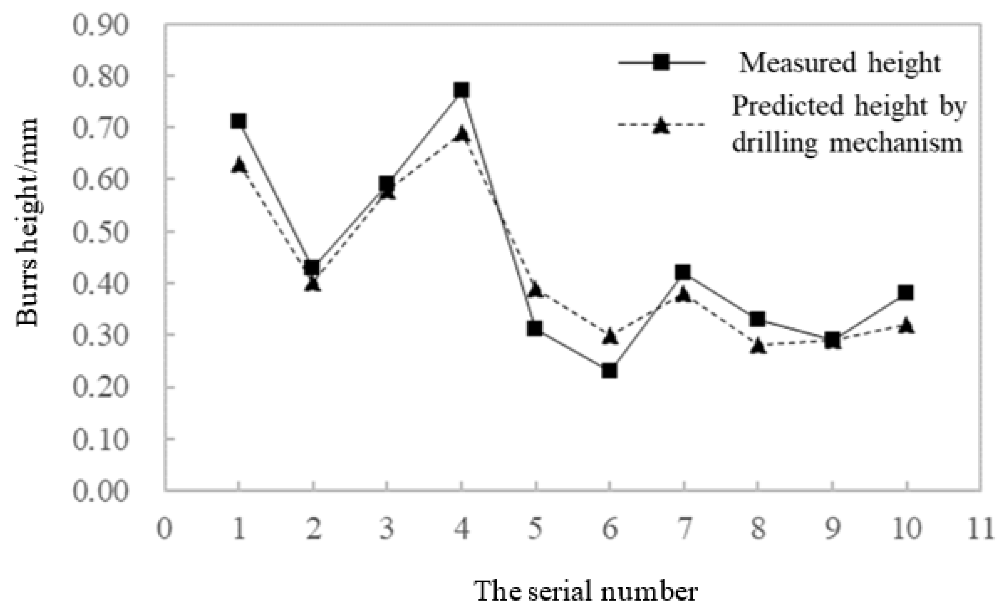
3.2. Prediction Mechanism Model of Drilling Burr Scale

The generation of burrs is closely related to the drilling depth and ductile fracture, usually occurring at the late unstable stage of the drilling process. Due to the impact of drilling speed and feed, burr formation can be divided into two situations: the tool penetrates the workpiece, and the tool does not penetrate workpiece [40,41]. This paper models these two kinds of burrs, respectively, and reconstructs the burrs in real environments through different energy combinations.
(1)
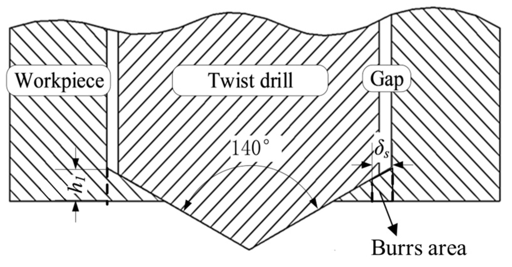
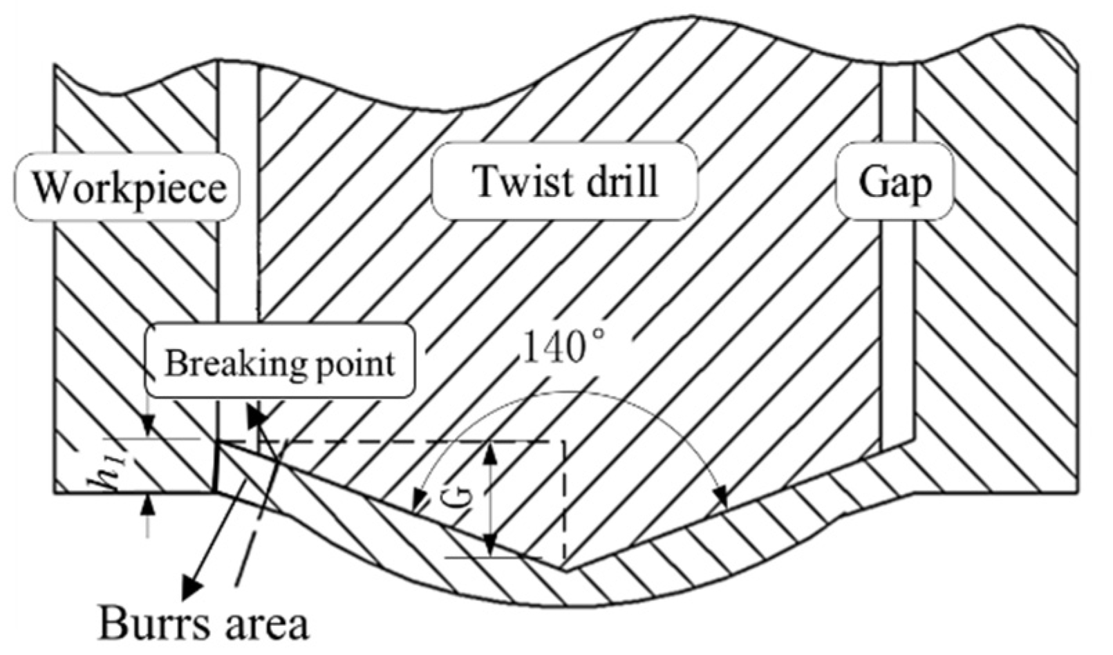
The tool penetrates workpiece: When the drill bit breaks through the workpiece material, the burr on the edge can be regarded as pure plastic deformation. Because of the radial vibration, there is an equivalent gap in the hole, similar to the blanking process, and this gap has a certain effect on the generation of burrs. As shown in Figure 3, assuming that the equivalent clearance is δs, which is equal to the amplitude of vibration, the expression of burr height Hpenetrate is shown in Equation (1) based on rigid plastic assumptions [42]. Figure 3 shows the h1 and δs schematics for the bit breaking through the workpiece material.
H p e n e t r a t e = K h | x z x x | ( r k δ s tan p 2 + h 1 r k δ s tan p 2 sin p 2 ) ( 1 Ψ 1 % )
where Hpenetrate is the burr height; Kh is the stiffness coefficient; xx is the forced vibration quantity in the x direction, and xz is the forced vibration quantity in the z direction; h1 is the maximum uncut thickness; r is the length of the bit cross edge; k = C/Vz, where C is the coefficient obtained in the experiment and Vz is the drilling feed rate; δs is equivalent gap; p is twist drill edge angle and generally takes p = 140°; and Ψ1 is the cross-section cutting rate of the workpiece material.
(2)
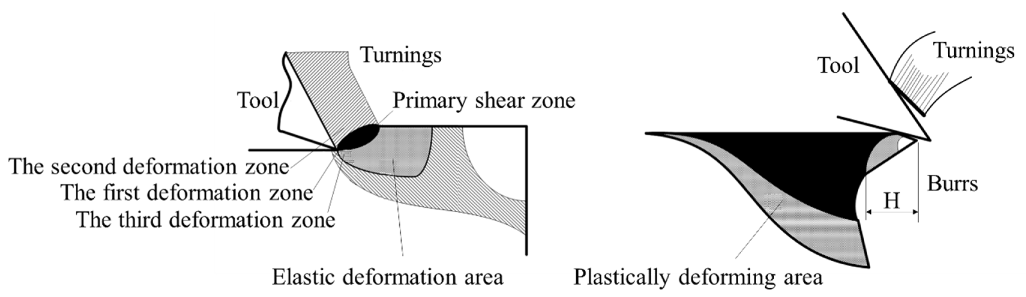
The tool does not penetrate the workpiece: At this point, the formation of burrs firstly appears as large plastic deformation and then as elastic fracture, as shown in Figure 4. Due to elastic backflow at the fracture [43], burr height only needs to be considered in terms of plastic elongation and the location of the danger point. At the moment before the workpiece material fracture, the strain rate εf reaches 0.3 to 0.5. At this point, the height curve of the burr edge can be approximately linearized. On this basis, the modified burr height H can be obtained by further considering the area shrinkage rate of material attributes, as shown in Equation (2).
H u n p e n e t r a t e = k δ s ε f 2 + 2 ε f K 1 e h 1 ( 1 Ψ 1 % )
where Hunpenetrate is the burr height; k = C/Vz, where C is the coefficient obtained in the experiment, and Vz is the drilling feed rate; δs′ is the equivalent gap; εf is the failure strain rate; K1 is axial stiffness; h1 is the maximum uncut thickness; and Ψ1 is the cross-section cutting rate of the workpiece material.
(3)
Equivalent height of burrs: The burr in real environments is the reconstruction of these two kinds of burrs under different energy ratios. The details are shown in Equation (3).
H m e c h a n i s m = K H 1 H p e n e t r a t e + K H 2 H u n p e n e t r a t e = K H 1 K h | X z X X | ( r k δ s tan p 2 + h 1 r k δ s tan p 2 sin p 2 ) ( 1 Ψ 1 % ) + K H 2 k δ s ε f 2 + 2 ε f K 1 e h 1 ( 1 Ψ 1 % )
where all parameters are consistent with those described in Equations (1) and (2); KH1 and KH2 are the energy reconstruction coefficients.

4. Error Compensation for Drilling Process by the Data-Driven Approach

There are many factors affecting weak rigid hole-making systems. The above mechanism model cannot accurately and comprehensively identify the influencing factors of drilling burr formation. Therefore, the rating results are subject to a large margin of errors. However, the data-driven method is a research hotspot in the industrial field, which can explore the relationship between data structures directly from the data itself without relying on prior knowledge. Therefore, the neural network model based on drilling data is introduced as a classification error compensation model, which is an effective means to modify the rating results of mechanism prediction.
Drilling state parameters are typical time series data; especially in the drilling exit stage, the vibration and drilling force signals have significant time series characteristics. According to this characteristic, a data-driven method for burr classification error discrimination considering multi-dimensional signal input is needed to make error analysis closely combined with drilling force and vibration signals and extract the hidden information behind the periodicity and correlation of different time nodes in signals [44]. The following content will involve several machine learning methods, which are defined as:
  • CNN: Convolutional Neural Network
  • RNN: Recurrent Neural Network
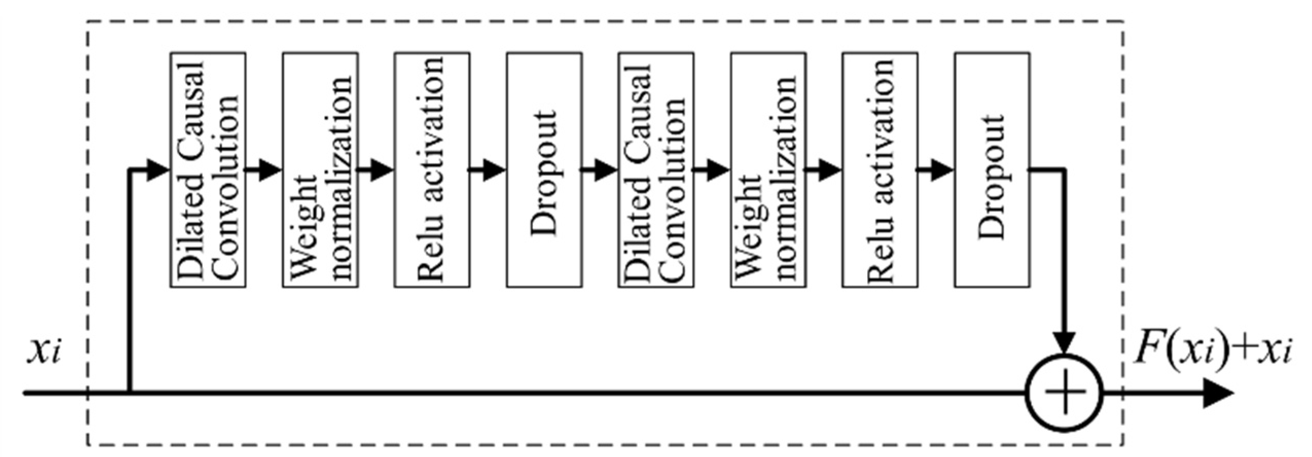
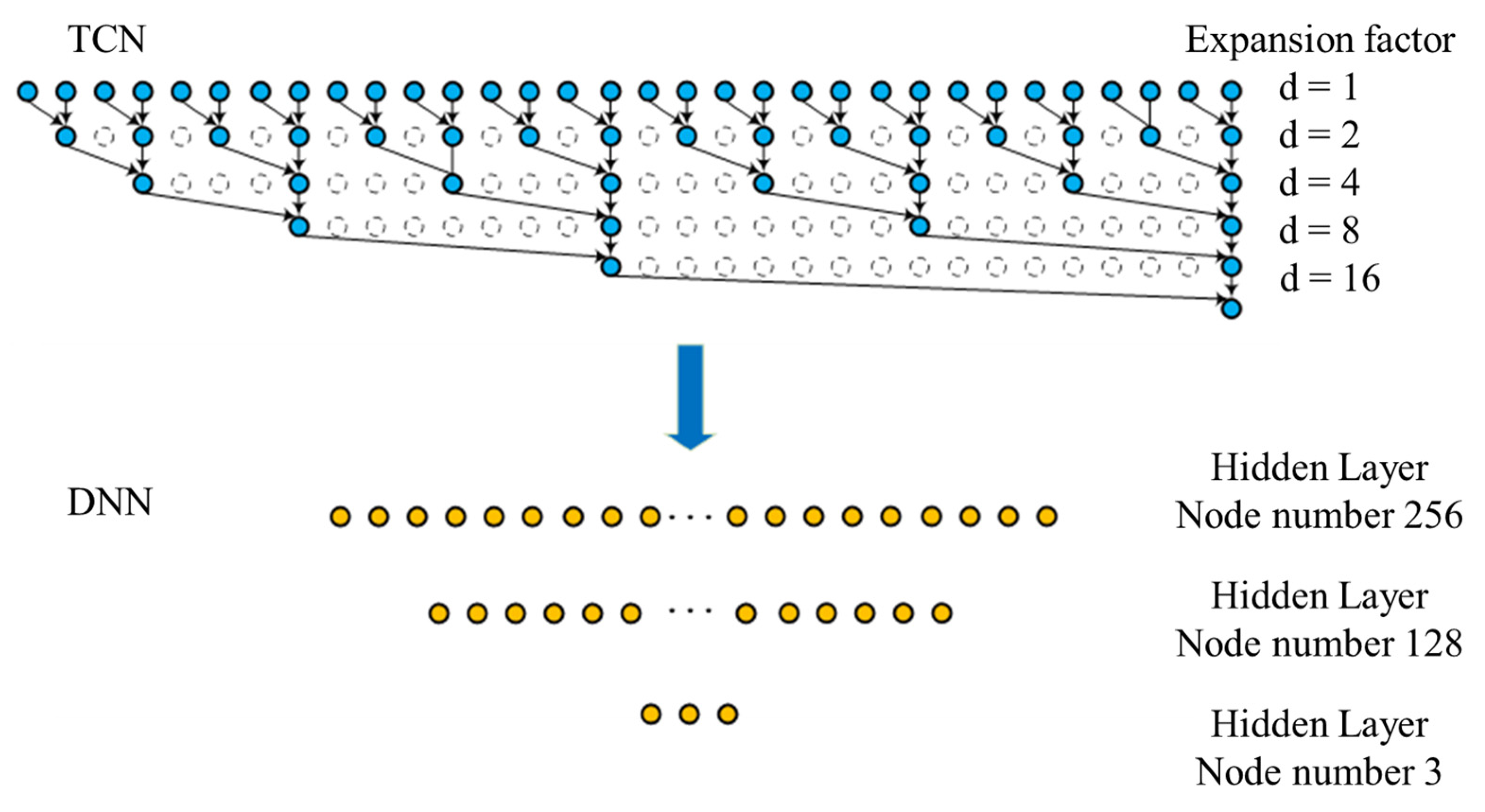
  • TCN: Temporal Convolutional Network
  • DNN: Deep Neural Network
  • TCN–DNN: Temporal Convolutional Network–Deep Neural Network
Drilling state parameters are the forms of typical two-dimensional inputs. The CNN is the typical prediction model to solve this problem, and the final prediction result can be obtained by convolution of two-dimensional information, or by virtue of RNNs, which serve as temporal prediction networks for the ultimate processing of two-dimensional data. However, due to the large time step of the dataset in the burr extrusion stage, traditional CNN and RNN training models will lead to the gradient disappearance of back propagation, which makes the corresponding model unable to learn. Therefore, the TCN is used as the substitute model of CNN and RNN in this paper to predict the error of data signals in the burr extrusion stage of the hole-making process.
The TCN convolution layer consists of four parts: causal cavity convolution, weight normalization, activation function, and dropout layer [45,46]. For the problem of long time series input, in order to minimize network depth and complexity and maximize the perception field, dilated causal convolution is adopted in the structure of the TCN model; at the same time, the weight normalization structure is added in TCN to avoid the gradient explosion when training the neural network; in addition, TCN uses Relu as the activation function, which can significantly reduce overfitting and computation; finally, according to the set probability, the dropout layer is added, and network units are randomly selected for propagation to reduce the training difficulty. The TCN network structure with two convolutional layers is shown in Figure 5.
Based on the TCN model, its network structure can be further expanded to make this model have stronger learning ability. The TCN–DNN model will be constructed by combining TCN with DNN. This model consists of two parts: the first part is TCN, the function of which is to extract the hidden information behind the periodicity of force and vibration signals and recognize the correlation of different time nodes in the hole-making stage; the second part is DNN, the function of which is to finally classify the mined information and form the error discrimination results [47]. In general, compared to some classical neural networks, such as CNN and RNN, TCN–DNN has more significant advantages, specifically as follows:
Firstly, there is a causal relationship between the layers of TCN. Historical information will affect the prediction of unknown data, and there will be no omissions. However, CNN and RNN models will constantly reduce the influence weight of untapped data, so that some information will be “forgotten”.
Secondly, the model architecture of TCN–DNN is highly adaptable to different data input scales and can also be modified according to the structural requirements of the data output.
Thirdly, TCN–DNN can ensure the parallelism of time series input, adjust the size of receiving domain flexibly, and ensure stable gradient, which can meet the requirements of data input under different time series lengths.
Fourthly, compared to a cyclic architecture with the same capacity, such as RNN, TCN saves more memory and reduces training requirements.

5. Fusion Modelling of Mechanism and Data

It is a new development direction for the fusion of mechanism and data to improve the prediction performance. In this section, a burr scale prediction architecture is proposed in which the mechanical characteristics of the drilling process are studied, and a data driven approach is used to perform multi-stage error compensation and correction.
The architecture of the weak rigid hole-making system designed in this paper is shown in Figure 6. Based on the burr-forming process, the machining state parameters, material properties of the workpiece, weak rigid system properties, nominal tool size, etc., should be comprehensively considered so as to determine the key parameters such as rated drilling force, rated torque, etc. In this study, the tool information includes its material and its geometric parameters (diameter, front angle, edge angle, etc.). The workpiece information includes the material and geometric size. The machining parameters include the terminal spindle speed (r/min) and feed rate (mm/s). The reading control of the working state for the end-effector communicates with the upper computer through a serial port. The state monitoring of the hole-making system is finally implemented.
The dynamic updated process is as follows: Firstly, the burr state is preliminarily evaluated based on the mechanism formula in the static physical model. Then the burr classification results can be preliminarily established referring to Table 1, where the classification and evaluation basis is shown. By comparing with the classification results of actual burr height, the difference between actual classification grade and theoretical calculating grade is worked out. These consequences are used as the label that serves as input for the error compensation model of the burrs. Moreover, the dynamic updated model takes force signals and machining parameters as inputs and determines whether the burr classification grade based on the mechanism formula needs to be increased, unchanged, or reduced. Finally, by training the network, the burr classified prediction in the weak rigid hole-making system based on the fusion of mechanism and data is realized. Furthermore, the final prediction result is the updated value of the data model acting on the mechanism model. That is, it is the sum of the prediction results of the mechanism model Y1 and the dynamic updated model Y2.
The state parameters of the drilling process are time series data, so a model with a better ability to extract time series information is needed. In this paper, the part of the neural network in the dynamic updated model adopts TCN–DNN to train the input data, where TCN is used to explore the timing regularity of processing state parameters, and DNN is used to classify the mined information, solving the problem of long-term dependence on data input.
Due to the huge information capacity of the original data after denoising, it cannot be directly used in the training of TCN–DNN. The burr state can be reflected only after its feature extraction and normalization. Therefore, the inputs of the dynamic updated model are the time-domain characteristic values of spindle speed, feed, three-component drilling force, and axial torque under the current hole-making conditions. The outputs are the differences between the actual classification grade of burr height and the theoretically calculated classification grade, that is, whether the prediction classification grade of real burrs needs to be increased or decreased.
It needs to be emphasized that the fusion model proposed in this paper is more suitable for burr classified prediction rather than parameters of real-time control of the drilling process. To achieve that, it is necessary to monitor the burr growth state and provide decision feedback according to the abnormal status information of burrs. This requires the establishment of a decision information base and optimization model library, which will be researched in the future.

6. Borehole Testing and Burr Scale Prediction

The fusion modeling method for burr classified prediction of the weak rigid drilling process was described in detail above. In this section, a drilling platform is designed and built. The method is further verified by a realistic case originating in a weak rigid hole-making system.

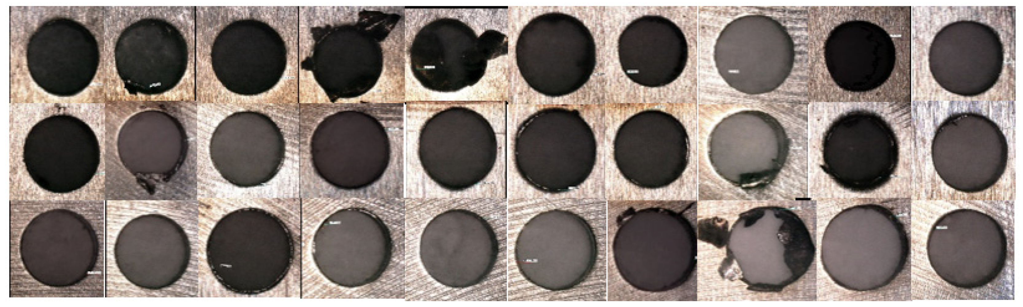
6.1. Experimental Design

In order to verify the advantages and effectiveness of the proposed method, a small automatic hole-making system with weak rigidity was designed independently, imitating the last joint of the robot. The drilling system consisted of a gantry frame, a power head, associated sensors, and other accessories, as shown in Figure 7.
(1)
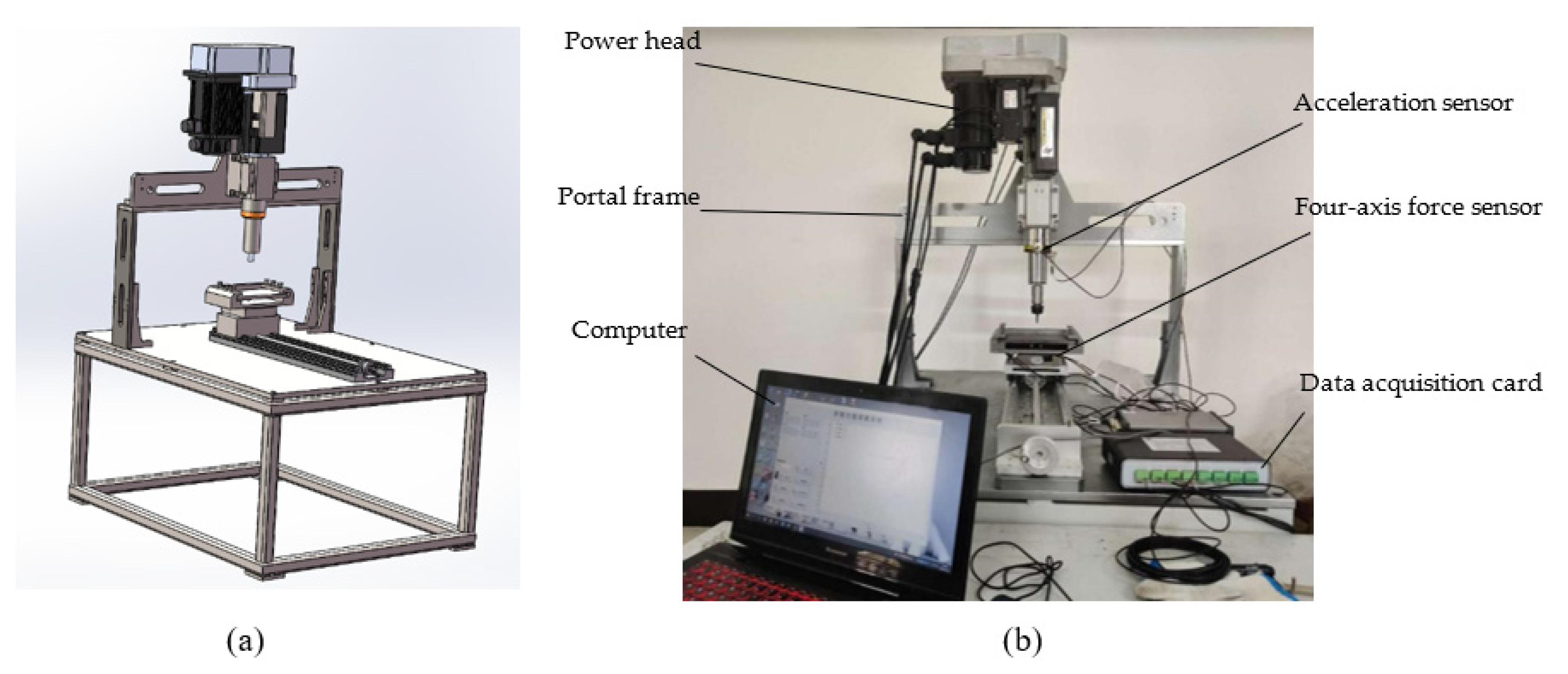
Frame: A self-designed gantry frame and a metal platform for installing the gantry frame were used. A one-dimensional slide table was installed on it to adjust the machining position of the experimental workpiece, so that a piece of workpiece could be tested many times, and reliable experimental results could be obtained.
(2)
Power head: A double servo tapping and drilling machine was selected and connected to the gantry frame through the installation base. A laser level meter and other related equipment were used to adjust the frame to ensure its shape and position deviation meets the requirements. The power head was controlled by a Galil control card, model is DMC-B140-M, which adopts the control mode of C# language of the upper computer. In addition, the spindle rotation servo motor used has a rated power of 1.8 kw and torque of 6 Nm. The feed servo motor used has a rated power of 0.4 kw and torque of 1.27 Nm.
(3)
Sensor: An acceleration sensor (INV3062T) was installed on the power head, and a four-axis sensor (NOS-C906) was mounted on the slide platform to collect the parameters of axial force and torque during the machining process. Its rated load was 1 KN/1 KN/2 KN/200 Nm, and its sensitivity was 1%.
(4)
Fixture: An ER20 collet was installed at the end of the power head with a 6 mm clip. By self-design, it was mounted on the four-axis sensor. Thus, the data collected by the sensor was more stable and reliable. An alloy steel straight shank twist drill was selected for the drilling tool.
The platform was suitable for drilling experiments with diameters of 6 mm and below. A #45 steel sheet of 200 mm × 100 m × 10 mm was selected as the workpiece material. Its strength limit was about 600 Mpa. The axial force and torque were collected by the four-axis sensor, and vibration signals were collected by the acceleration sensor. These data were used to predict the scale rating of drilling burrs in weak rigid systems. The main component parameters are shown in Table 2. Please refer to Appendix A for more detailed technical parameters.
In order to obtain the stiffness and natural frequency of the system, ABAQUS was used for finite element analysis in this paper. The axial stiffness of the system was 8,571,429 N/m by simulation, and the radial stiffness was 4,137,932 N/m. The axial natural frequency was 34 Hz, and the radial natural frequency was 67 Hz. The system stiffness was about one tenth of that of machine tools with the same specifications, which proved that the system was weakly rigid.
Data of burr height was collected in the experiment. As the burr edge appeared to be tearing, the workpiece was firstly cut by wire cutting; Secondly, in order to describe the burr height comprehensively, six points on the burr were sampled by spiral micrometer on average. Finally, the mean value of sampling points was used as the experimental data of burr height.
Figure 8 shows part of the burrs in the real machining environment. The experimental results illustrated that the machining quality of the weak rigid drilling system was poor. It was easy to cause burrs at the outlet. Therefore, an accurate modelling method was needed to predict the burr grade in the machining process so as to provide a judgment basis for the burr post-treatment and to further implement the optimal state control in the machining process.

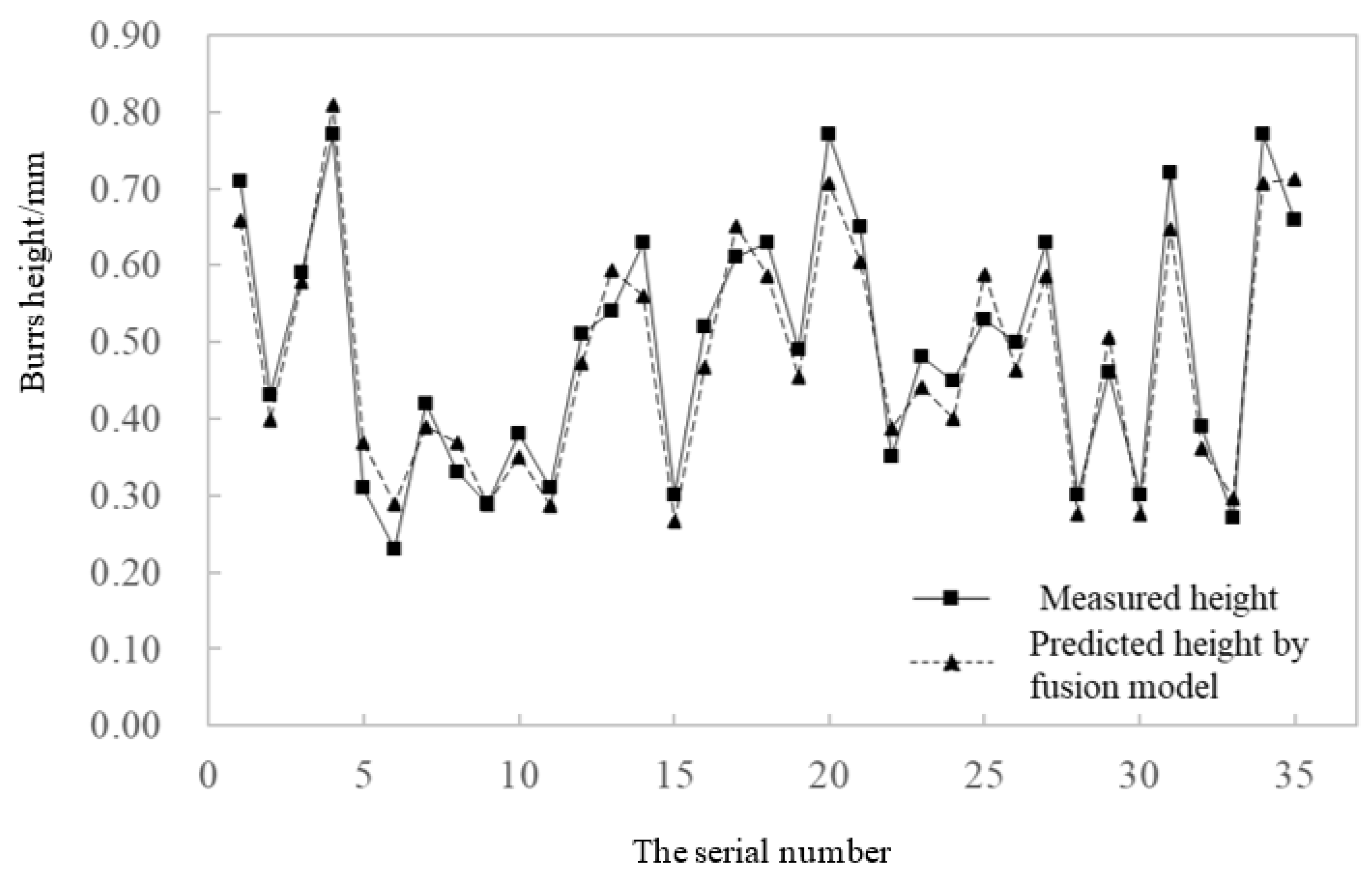
6.2. Predictive Analytics

In this paper, a straight shank twist drill made of alloy steel was used to drill 6 mm holes in #45 steel. A four-axis force sensor was used to collect the force signal, and the acceleration sensor was used to collect the vibration signal during the drilling process. Feature extraction was performed on the collected signals, and the drilling mechanism model was used to predict the burr height to verify the validity of the traditional model. The experimental results and theoretical predicted values were investigated, as shown in Figure 9. Part of the experimental and predicted results of burr height are shown in the figure. The comparison results showed that the mechanism model adopted in this paper had a certain burr prediction ability. The average error between measured values and predicted values based on the drilling mechanism was 12%. However, it was also observed that the maximum prediction error reached nearly 30%, which showed that there was still great inconsistency. This result shows the limitation of the pure mechanism model. Faced with masses of uncertain factors affecting the drilling performance, it is almost impossible to build an analytical model that can accurately predict the burrs.
In addition, an effective error compensation model based on the fusion of machine learning techniques was established, which involved TCN and DNN. On the basis of the above experiments, further feature collection was carried out on the boreholes in the experiment, and the burr characteristics were classified. The error results are shown in Table 3. By comparing the actual burr classification grade with the burr classification grade calculated based on mechanism model, the corresponding error label could be obtained. According to the processing dataset of the time-series feature, and the labeled dataset consisting of burr evaluation data measured in the experiment, the results were randomly classified. The label value of the dataset was the grade error of burr evaluation between the actual measured value and the theoretical value. The top 10 groups of specific experimental evaluation grade errors are shown in Table 3.
The TCN–DNN model was constructed, as shown in Figure 10. The input signal structure was x, and its size was 500 × 42; 500 represented 500 truncations analyzed in the time–frequency domain, and 42 meant 6 times 7, i.e., there were 6 signal types in total, and 7 time–frequency domain features were obtained for each signal. The output results were three classification results, whose meanings were: increase the burr rating, not change the burr rating, and reduce the burr rating.
The parameter settings of the TCN–DNN model are shown in Table 4. The dropout layer coefficient was set to 0.5 in the model to reduce the impact of data fluctuations. The Softmax activation function was applied to multi-category scenarios, and the vector dimension could be reduced to three dimensions with its help. This was because there were three categories to predict in the model: to increase the burr rating, to not change the burr rating, and to reduce the burr rating.
Figure 11 shows the prediction results corrected by TCN–DNN error compensation and the physical experimental results. As can be seen from Figure 11, the predicted values of the fusion model were in better agreement with the experimental values. The average relative error was about 9%. As can be seen from Figure 9 and Figure 11, the prediction accuracy of the fusion model improved by 25% compared with the results of the traditional drilling mechanism model. Due to the complexity of weak rigid hole-making systems, the prediction and classification effects of the pure mechanism model was poor, which could not directly meet the requirements of actual prediction accuracy. This result further illustrated the accuracy and reliability of the proposed burr classified prediction method. The fusion model integrates the burr formation mechanism and data-driven error compensation model, which can take advantage of both approaches and fully consider the mechanical characteristics of the drilling process. Therefore, using the TCN–DNN neural network to compensate and modify the traditional mechanism model is an effective means to improve the prediction performance of drilling burrs.
In order to further evaluate the advantages of the TCN–DNN model, the CNN model represented by VGGNET (Visual Geometry Group NET) and the traditional DNN model were selected as the control to calculate the convergence and loss values of the three models. The models were trained and tested under the same conditions: the hardware environment was an Intel i7-4770 + Nvidia GTX750, and the software environment was Windows 10 + Python 3.6 + Keras. Loss values of different models after training are shown in Figure 12.
It can be seen that the DNN model converged the fastest, but its loss value finally fluctuated around 0.85, which was much higher than that of the TCN–DNN and CNN model. However, the CNN model, using VGGNET, had the slowest convergence, and the loss result was also higher than that of the TCN–DNN model. To sum up, although the TCN–DNN model converged at the 38th iteration, the convergence speed of which ranked second, its loss value was the lowest, reflecting its best convergence. It can be seen that the optimal iteration number of TCN–DNN model was 40 times. Moreover, the prediction results based on the TCN–DNN model had the highest accuracy, reaching 91.67%, higher than that of the traditional CNN and DNN networks. This was determined by the characteristics of the TCN–DNN network. There was a causal relationship between the layers of the time convolutional network; that is, historical information could affect the unknown data prediction, and there would be no omission. This accuracy rate further proved that the TCN–DNN model can be applied to complex burr classification and prediction scenarios.
Based on the above comparative analysis, it can be seen that TCN–DNN has more significant advantages. Experimental results prove that this trained network has fully explored the timing regularity of machining state parameters and can both accurately harmonize the past data and precisely predict the burr quality. To be specific, compared to the classical neural networks, such as CNN and RNN, TCN–DNN can ensure the parallelism of time series input, adjust the size of receiving domain flexibly, and ensure a stable gradient, which can meet the requirements of data input under different time series lengths.
In addition, the TCN–DNN model and its classification tasks will be further taken into consideration comprehensively. Optimizers often play an important role in machine learning. The performance of the same model may differ greatly due to the selection of different optimizers, and even some models cannot be trained. In this experiment, three optimizers including Adam, RMSprop, and SGD were selected for comparison. The influence of different learning rates on model accuracy and convergence speed were synchronously investigated.
Specifically, SGD adopts the stochastic gradient descent algorithm. This solver generally uses a small batch gradient descent algorithm in training; that is, it selects part of the data for training. This gradient-updating algorithm is concise and can converge to the globally optimal solution (convex function) or locally optimal solution (non-convex function) when the learning rate is appropriately designed. However, the solver is sensitive to the hyperparameter learning rate and is easy to misjudge. Thus, the model will end the iteration before reaching the extreme point and fall into the local minimum.
RMSProp is an effective and practical deep neural network optimization algorithm. It can automatically adjust the learning rate of model parameters independently and update sparse parameters greatly and frequent parameters slightly. Therefore, the RMSProp method is very suitable for processing sparse data. However, there are still some deficiencies, such as the premature or excessive reduction of the learning rate, which is caused by the cumulative gradient square.
Adam is essentially RMSProp with momentum terms, which dynamically adjust the learning rate of each parameter using the first and second moment estimation of the gradient. The advantages of this optimizer mainly lie in the fact that after bias correction, the learning rate of each iteration has a certain range, which makes the parameters more stable. In addition, Adam is suitable for scenarios with large-scale data and parameters applied to the unstable objective function.
Simulation results showed that the influence of different learning rates on model accuracy and convergence speed was significantly different. Through experimental comparison, Adam had the best effect, and its test accuracy reached 91.67%, as shown in Figure 13. Therefore, the Adam optimizer could be used to ensure the best prediction accuracy of burrs in weak rigid hole-making systems.
To be sure, the creation of an efficient and sustainable processing mode is critical. At present, multivariant industrial robots have been widely used in automatic production lines, welding manufacturing, material handling, and other application scenarios with high renaturation. Moreover, industrial robots are also gradually being adopted in aerospace and military industries, automobile manufacturing, and other fields to replace humans. The experimental platform built in this paper serves as a prototype system to simulate the drilling process in real industrial applications. Experimental results demonstrated the effectiveness and feasibility of the proposed method. This basic research about algorithm design and optimization is currently being focused, and practical industrial applications are expected in the future.

7. Conclusions

This article attempts to establish a fusion model for burr classified prediction in a weak rigid hole-making system. On the one hand, the expressions of burr characteristics are deduced based on vibration mechanisms, and the preliminary classification results are calculated; on the other hand, according to the measured data, the errors between initial calculation results and actual classification results are obtained and selected as the tag values of the dataset. Finally, by training the network of TCN–DNN using the drilling data, the burr classified prediction based on the fusion model is realized. The following conclusions can be drawn:
(1)
The proposed burr classified prediction method can integrate the burr formation mechanism and data-driven error compensation model, which fully considers the mechanical characteristics of the drilling process. The overall calculation accuracy has improved by 25% compared with that of the traditional drilling mechanism model.
(2)
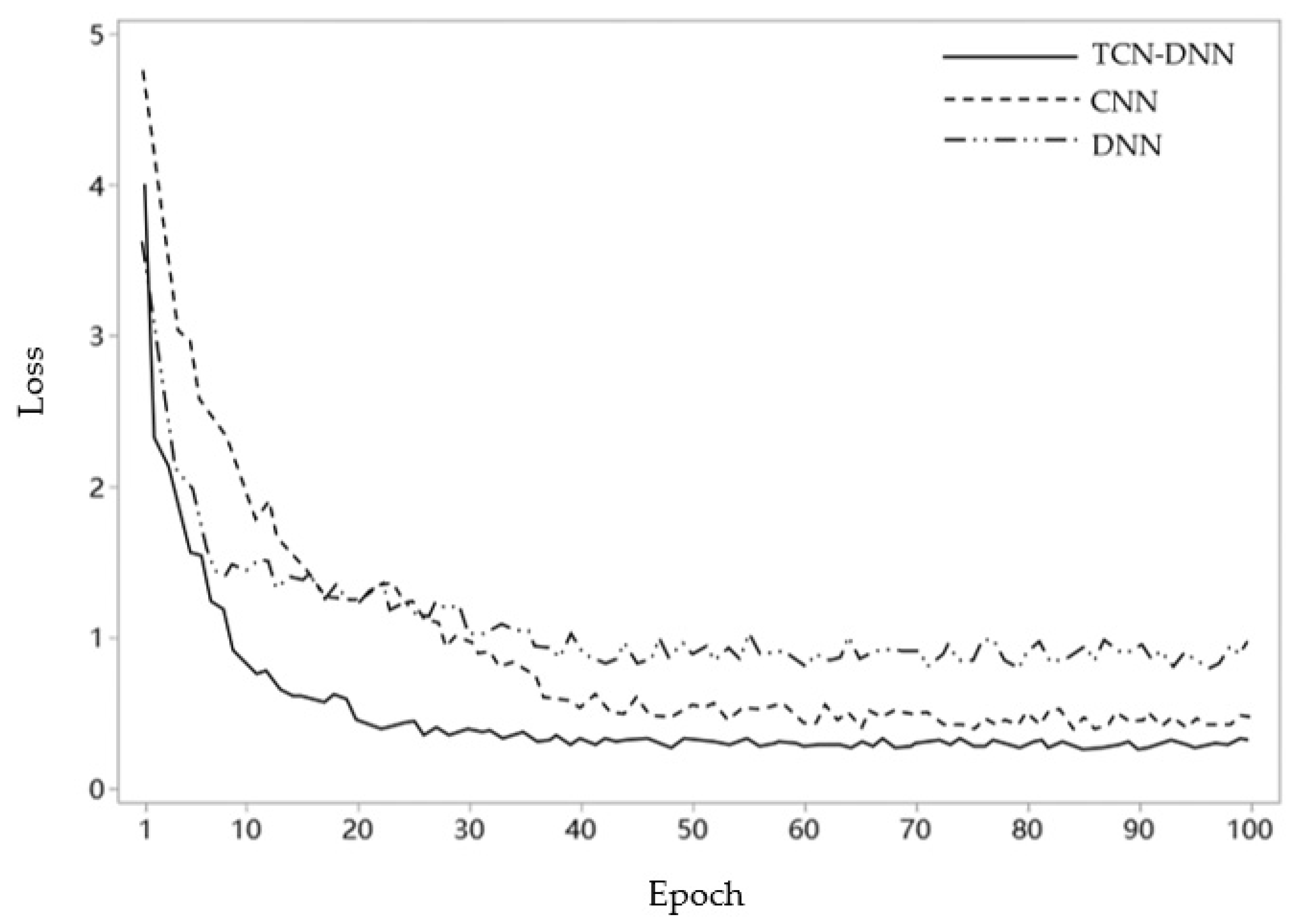
An effective error compensation model based on the fusion of machine learning techniques is established, which involves the temporal convolutional network and deep neural network. The trained network fully explores the timing regularity of machining state parameters and can both accurately harmonize the past data and precisely predict the burr quality. The algorithm has the highest accuracy, reaching 91.67%, which is higher than that of traditional networks, and a satisfactory convergence speed.
(3)
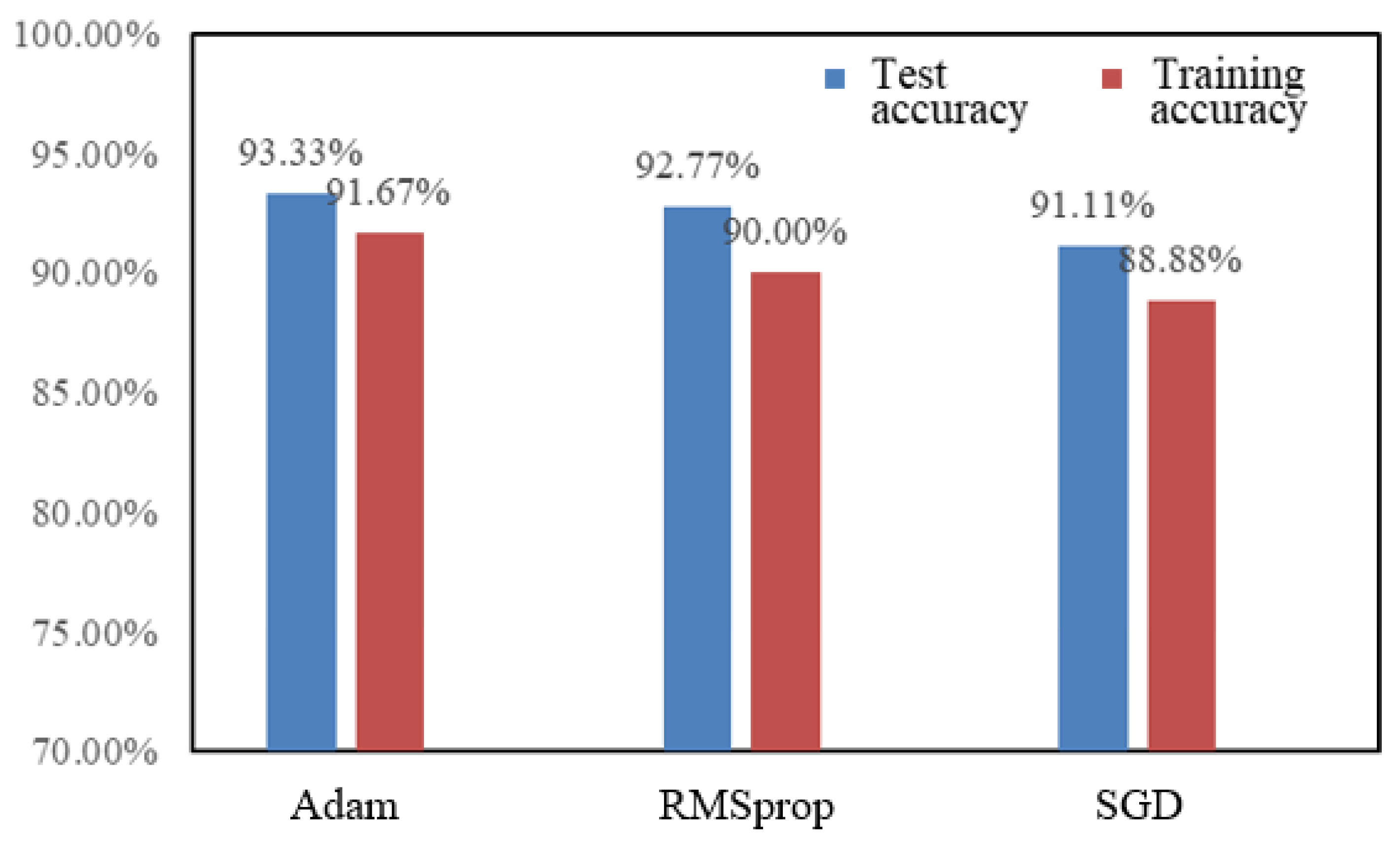
The accuracy and feasibility of the proposed method are further verified by a realistic case originating in a weak rigid hole-making system. Experimental results show that the Adam optimizer has the best prediction accuracy and can be adopted in the proposed prediction model. The research has strong practical significance and theory-guiding sense. It can be widely used in automatic hole-making systems, such as in aerospace, military, and other fields.
However, there are also some deficiencies in this method. The fusion model is still overly machining environment-dependent, and certain errors will appear for different processing scenarios (different types of cutting tools, different processing materials, etc.). Moreover, the fusion model is more suitable for burr classified prediction rather than real-time parameter control of the drilling process. To achieve this, the establishment of a decision information base and optimization model library is required. In the future, the idea of transfer learning could be integrated into this model to increase the generalization capability of the fusion model, making it not overly dependent on the processing environment. On the other hand, the state monitoring in the machining process should be focused in order to further realize the real-time optimal control for the drilling process.

Author Contributions

Writing—original draft preparation, S.D., Q.Y.; writing—review and editing, X.Z., M.W.; funding acquisition, S.D., X.Z. All authors have read and agreed to the published version of the manuscript.

Funding

This work was financially supported by the grants from the National Natural Science Foundation of China (Grant Nos. 51805079 and 52105509), and the Fundamental Research Funds for the Central Universities under Grant Numbers 2232021D-15 and 2232019D3-33. The authors are grateful for these financial supports.

Conflicts of Interest

The authors declare no conflict of interest.

Appendix A

Table A1. Technical parameters of motion controller DMC-B140-M.
ParameterIndex
System processor32-bit MPU
Flash EEPROM
RAM
Communication interfaceEthernet 100BASE-T
RS232 115.2K
Mode of motionPoint-to-point positioning control
Location tracking
JOG
2D line/arc interpolation with feed multiplier
1–4 axis linear interpolation
Electronic gear control with multiple driving shafts
Synchronism of gate bridge
Electronic cam
Contour control
S-curve acceleration and deceleration
Memory function450 lines × 40 characters
126 variables
800 elements in 6 arrays
Range of motionPosition: 32 bits
Speed: 32 bits
Acceleration: 32 bits
Universal digital I/O8 inputs/4 outputs
High-speed set latch4-way latch input for X, Y, Z, W axis
Private inputMaster encoder input: A, A−, B, B−, I, I−; +/−12 V
Positive and negative limit input
Back to zero input
High-speed position latch input
Emergency stop input
Private outputInstruction pulse and direction output for stepper motor
Servo enable output
Signal transfer output
Minimum servo updating rate1–2 axis: 125 us
3–4 axis: 250 us
Maximum encoder feedback rate12 MHZ
Maximum step forward motor command rate3 MHZ
Power source specification19–33VDC, ≥0.5 A
Work environmentWorking temperature: 0–70 °C
Humidity: 20–95% RH
Table A2. Technical parameters of acceleration sensor INV3062T.
ParameterIndex
Analog
input
Number of channels2–4
AD precision:24 bits or double 24 bits (double core)
Maximum sampling frequency51.2 KHz for each channel
Frequency indication and resolution error<0.01%
Spectrum amplitude error<1%
Dynamic range of 24 bits channel120 dB (typical value), 110 dB (guaranteed value)
Dual-core channel range160 dB
Input range of 24 bits channel10 V, 1 V, 0.1 V
Dual-core channel input range10 V for one gear only (range: 160 dB)
Input noise of 24 bits channel<0.05 m Vrms @ ±10 V range (typical value 0.03 m Vrms)
Dual-core channel input noise<0.005 m Vrms @ ±10 V range (typical value 0.003 m Vrms)
Anti-aliasing filter256 times oversampling + digital filter + analog anti-aliasing filter, the total attenuation steepness is over −300 dB/oct
Total harmonic distortion−70 dB
Interchannel crosstalk−100 dB
Input impedance>1MΩ
Input modeVoltage DC, voltage AC, IEPE(ICP)
External conditioning unitCharge, strain
Rpm
input
Tacho
Number of channels0–1
Internal sampling rate25 MHz, supporting torsional vibration measurement
Rotary speed range3–3,000,000 rpm
Input voltage range−5 to +5 VDC
InterfaceLEMO three-core connector, can supply power of +5 V to photoelectric sensor
Digital
input/
output
system
ModeRS232
Number of channels0–1
Cascade
connection
Number of cascade acquisition instrumentsStandard: 1–8 sets; customize: 9–32 or more
Cascade synchronization between instrumentsSynchronous cable RJ45 twisted pair cable, maximum 100 m; built-in GPS module, external antenna
Table A3. Technical parameters of force sensor NOS-C906.
ParameterIndex
Rated output1.0 mV/V ± 0.1%
Zero balance±1% of rated output
Creep after 30 min±0.5% of rated output
Nonlinearity±0.5% of rated output
Hysteresis±0.5% of rated output
Repeatability±2.0% of rated output
Temp. effect on output≤0.02% of applied output/°C
Temp. effect on zero≤0.02% of applied output/°C
Safe temp. range−10 °C to +70 °C
Temp. compensated−10 °C to +40 °C
Safe overload150%
Input impedance387 ohm ± 20 ohm
Output impedance350 ohm ± 5 ohm
Rated excitation10 V DC/AC
Maximum excitation15 V DC/AC

References

  1. Bi, S.; Liang, J. Robotic drilling system for titanium structures. Int. J. Adv. Manuf. Tech. 2011, 54, 767–774. [Google Scholar] [CrossRef]
  2. Cen, L.; Melkote, S.N.; Castle, J.; Appelman, H. A wireless force-sensing and model-based approach for enhancement of machining accuracy in robotic milling. IEEE/ASME Trans. Mechatron. 2016, 21, 2227–2235. [Google Scholar] [CrossRef]
  3. Zeng, Y.; Tian, W.; Liao, W. Positional error similarity analysis for error compensation of industrial robots. Robot C. Int. Manuf. 2016, 42, 113–120. [Google Scholar] [CrossRef]
  4. Bu, Y.; Liao, W.; Tian, W.; Zhang, J.; Zhang, L. Stiffness analysis and optimization in robotic drilling application. Precis. Eng. 2017, 49, 388–400. [Google Scholar] [CrossRef]
  5. Huang, J.; Xiong, Y.; Huang, J.; Wang, G. Finite element analysis of burr formation in micro-machining. Appl. Mech. Mater. 2014, 487, 225–229. [Google Scholar] [CrossRef]
  6. Huang, J.; Zhu, Y.; Li, Q.; Wang, G. Active control methods of cutting burr in precision and ultra-precision machining. Appl. Mech. Mater. 2014, 494–495, 620–623. [Google Scholar] [CrossRef]
  7. Zai, P.; Tong, J.; Liu, Z.; Zhang, Z.; Song, C.; Zhao, B. Analytical model of exit burr height and experimental investigation on ultrasonic-assisted high-speed drilling micro-holes. J. Manuf. Proc. 2021, 68, 807–817. [Google Scholar] [CrossRef]
  8. Zheng, X. Key Technology and Fundamental Research of Micro-Drilling and Micro-Milling. Ph.D. Thesis, Shanghai Jiao Tong University, Shanghai, China, 2013. [Google Scholar]
  9. Mondal, M.S.; Mandal, M.C. FPA based optimization of drilling burr using regression analysis and ANN model. Measurement 2020, 152, 107327. [Google Scholar] [CrossRef]
  10. Jia, Z.; Zhang, C.; Wang, F.; Fu, R.; Chen, C. An investigation of the effects of step drill geometry on drilling induced delamination and burr of Ti/CFRP stacks. Compos. Struct. 2020, 235, 111786. [Google Scholar] [CrossRef]
  11. Kwon, B.; Mai, N.D.D.; Cheon, E.S.; Ko, S.L. Development of a step drill for minimization of delamination and uncut in drilling carbon fiber reinforced plastics (CFRP). Int. J. Adv. Manuf. Tech. 2020, 106, 1291–1301. [Google Scholar] [CrossRef]
  12. Hassan, A.A.; Soo, S.L.; Aspinwall, D.K.; Arnold, D.; Dowson, D. An analytical model to predict interlayer burr size following drilling of CFRP-metallic stack assemblies. Cirp. Ann. Manuf. Technol. 2020, 69, 109–112. [Google Scholar] [CrossRef]
  13. Hu, L.; Zheng, K.; Dong, S. Burr characteristics of robotic rotary ultrasonic drilling aluminum alloy stacked components. J. Beijing Univ. Aeronaut. Astronaut. 2020, 46, 407–413. [Google Scholar]
  14. Li, S.; Zhang, D.; Liu, C.; Tang, H. Exit burr height mechanistic modeling and experimental validation for low-frequency vibration-assisted drilling of aluminum 7075-T6 alloy. J. Manuf. Proc. 2020, 56, 350–361. [Google Scholar] [CrossRef]
  15. Yang, F.; Xing, Y.; Li, X. A comprehensive error compensation strategy for machining process with general fixture layouts. Int. J. Adv. Manuf. Tech. 2020, 107, 2707–2717. [Google Scholar] [CrossRef]
  16. Chen, B.; Chen, X.; Li, B.; He, Z.; Cao, H.; Cai, G. Reliability estimation for cutting tool based on logistic regression model. J. Mech. Eng. 2011, 47, 158–164. [Google Scholar] [CrossRef]
  17. Gebraeel, N.; Lawley, M. A neural network degradation model for computing and updating residual life distributions. IEEE Trans. Autom. Sci. Eng. 2008, 5, 154–163. [Google Scholar] [CrossRef]
  18. Yang, Y.; Zhang, B.; Liu, Q. Analysis and comparison of various cutting force models in the milling process simulation. J. Vib. Eng. 2015, 28, 82–90. [Google Scholar]
  19. Chang, D.; Pang, J.; Pan, J. Dynamics modeling of deep hole processing based on boring and trepanning association. Sci. Technol. Eng. 2014, 14, 216–219. [Google Scholar]
  20. Zheng, X.; Dong, D.; Huang, L.; An, Q.; Wang, X.; Chen, M. Research on fixture hole drilling quality of printed circuit board. Int. J. Precis. Eng. Man. 2013, 14, 525–534. [Google Scholar] [CrossRef]
  21. Xavier, R.; Francois, C.J.; Ewa, K.S.J.; Marek, B. Burr height monitoring while drilling CFRP/ titanium/aluminium stacks. Mech. Ind. 2017, 18, 114–125. [Google Scholar]
  22. An, Q.; Tao, Z.; Xu, X.; Mansori, M.E.; Chen, M. A data-driven model for milling tool remaining useful life prediction with convolutional and stacked LSTM network. Measurement 2020, 154, 107461. [Google Scholar] [CrossRef]
  23. Xu, X.; Tao, Z.; Ming, W.; An, Q.; Chen, M. Intelligent monitoring and diagnostics using a novel integrated model based on deep learning and multi-sensor feature fusion. Measurement 2020, 165, 108086. [Google Scholar] [CrossRef]
  24. Dahl, G.E.; Yu, D.; Deng, L.; Acero, A. Context-dependent pre-trained deep neural networks for large-vocabulary speech recognition. IEEE Trans. Audio Speech Lang. Processing 2011, 20, 30–42. [Google Scholar] [CrossRef] [Green Version]
  25. Montavon, G.; Samek, W.; Müller, K. Methods for interpreting and understanding deep neural networks. Digit. Signal Proc. 2018, 73, 1–15. [Google Scholar] [CrossRef]
  26. Abd-Elwahed, M.S. Drilling process of GFRP composites: Modeling and optimization using hybrid ANN. Sustainability 2022, 14, 6599. [Google Scholar] [CrossRef]
  27. Gaitonde, V.N.; Karnik, S.R. Minimizing burr size in drilling using artificial neural network (ANN)-particle swarm optimization (PSO) approach. J. Intell. Manuf. 2012, 23, 1783–1793. [Google Scholar] [CrossRef]
  28. Gan, M.; Wang, C.; Zhu, C.A. Construction of hierarchical diagnosis network based on deep learning and its application in the fault pattern recognition of rolling element bearings. Mech. Syst. Signal Pr. 2016, 72–73, 92–104. [Google Scholar] [CrossRef]
  29. Wang, J.; Ye, L.; Gao, R.; Li, C.; Zhang, L. Digital Twin for rotating machinery fault diagnosis in smart manufacturing. Int. J. Prod. Res. 2019, 57, 3920–3934. [Google Scholar] [CrossRef]
  30. Yu, J.; Song, Y.; Tang, D.; Dai, J. A Digital Twin approach based on nonparametric Bayesian network for complex system health monitoring. J. Manuf. Syst. 2020, 2020, 293–304. [Google Scholar] [CrossRef]
  31. Booyse, W.; Wilke, D.N.; Heyns, S. Deep digital twins for detection, diagnostics and prognostics. Mech. Syst. Signal Pr. 2020, 140, 106612. [Google Scholar] [CrossRef]
  32. Luo, W.; Hu, T.; Ye, Y.; Zhang, C.; Wei, Y. A hybrid predictive maintenance approach for CNC machine tool driven by Digital Twin. Robot C. Int. Manuf. 2020, 65, 101974. [Google Scholar] [CrossRef]
  33. Wang, C.; Erkorkmaz, K.; Mcphee, J.; Engin, S. In-process digital twin estimation for high-performance machine tools with coupled multibody dynamics. Cirp. Ann.-Manuf. Technol. 2020, 69, 321–324. [Google Scholar] [CrossRef]
  34. Hu, F.; Yang, Y.; Liu, S.; Zheng, X.; Lv, X.; Bao, J. Digital twin high-fidelity modeling method for spinning forming of aerospace thin-walled parts. CIMS 2022, 28, 1282–1292. [Google Scholar]
  35. Liu, J.; Zhao, P.; Zhou, H.; Liu, X.; Feng, F. Digital twin-driven machining process evaluation method. CIMS 2019, 25, 1600–1610. [Google Scholar]
  36. Liu, S.; Bao, J.; Lu, Y.; Li, J.; Lu, S.; Sun, X. Digital twin modeling method based on biomimicry for machining aerospace components. J. Manuf. Syst. 2021, 58, 180–195. [Google Scholar] [CrossRef]
  37. Han, G.; Pan, G.; Wu, W.; Xu, L. Research on the burr forming characteristics of ultrasonic assisted micro-milling process. J. B Inst Technol. 2018, 38, 888–892. [Google Scholar]
  38. Zaeh, M.; Roesch, O. Improvement of the machining accuracy of milling robots. Prod. Eng. 2014, 8, 737–744. [Google Scholar] [CrossRef]
  39. Huang, J.; Huang, J.; Yang, C.; Wang, G. Development research on micro-machining burr. Mach. Des. Manuf. 2014, 7, 256–258. [Google Scholar]
  40. Wu, D.; Huang, S.; Gao, Y.; Dong, Y.; Ma, X. Predictive model for the interlayer burr height during drilling of stacked aluminum plates. J. Tsinghua Univ. Sci. Technol. 2017, 57, 591–596, 603. [Google Scholar]
  41. Hu, Y.; Song, Y.; Li, Y.; Yao, Z. An analytical model to predict interfacial burr height for metal stack drilling. Proc. Inst. Mech. Eng. Part B 2019, 233, 99–108. [Google Scholar] [CrossRef]
  42. Sachnik, P.; Hoque, S.E.; Volk, W. Burr-free cutting edges by notch-shear cutting. J. Mater. Proc. Tech. 2017, 249, 229–245. [Google Scholar] [CrossRef]
  43. Régnier, T.; Fromentin, G.; Marcon, B.; Outeiro, J.; D’Acunto, A.; Crolet, A.; Grunder, T. Fundamental study of exit burr formation mechanisms during orthogonal cutting of AlSi aluminium alloy. J. Mater. Proc. Tech. 2018, 257, 112–122. [Google Scholar] [CrossRef] [Green Version]
  44. Zhou, W.; Liao, W.; Tian, W. Theory and experiment of industrial robot accuracy compensation method based on spatial interpolation. J. Eng. Mech. 2013, 49, 42–44. [Google Scholar] [CrossRef]
  45. Gao, X.; Ma, D.; Han, H.; Gao, H. Fault prediction of complex industrial process based on DAE and TCN. Chin. J. Sci. Instrum. 2021, 42, 140–151. [Google Scholar]
  46. Shi, H.; Liu, X.; Xiao, Q. Improved temporal convolutional networks for sequential recommendation. J. Chin. Comput. Syst. 2021, 42, 1382–1388. [Google Scholar]
  47. Tsironi, E.; Barros, P.; Weber, C.; Wermter, S. An analysis of convolutional long short-term memory recurrent neural networks for gesture recognition. Neurocomputing 2017, 268, 76–86. [Google Scholar] [CrossRef]
Figure 1. Burr formation mechanism and characteristic parameters.
Sustainability 14 07429 g001
Figure 2. Actual burr classification: (a) level 1, (b) level 2, and (c) level 3.
Sustainability 14 07429 g002aSustainability 14 07429 g002b
Figure 3. Drilling process for the tool-penetrating workpiece.
Sustainability 14 07429 g003
Figure 4. Drilling process for the tool un-penetrating workpiece.
Sustainability 14 07429 g004
Figure 5. The structure of TCN.
Sustainability 14 07429 g005
Figure 6. Burr classified prediction model architecture.
Sustainability 14 07429 g006
Figure 7. Drilling platform: (a) virtual prototype, and (b) experimental platform.
Sustainability 14 07429 g007
Figure 8. Part of the drilling burrs at the outlet.
Sustainability 14 07429 g008
Figure 9. Burr height comparison between measured value and the predicted value based on the drilling mechanism.
Sustainability 14 07429 g009
Figure 10. TCN–DNN structure.
Sustainability 14 07429 g010
Figure 11. Burr height comparison between measured and predicted values based on the fusion model.
Sustainability 14 07429 g011
Figure 12. Loss assessment results after training.
Sustainability 14 07429 g012
Figure 13. Prediction accuracy of different optimizers.
Sustainability 14 07429 g013
Table 1. Burr classification and evaluation.
LevelBurr Height Ratio
(Burr Height/Material Thickness)
Rating Instructions
Level 1<5%This rating may be deemed not to require deburring operations.
Level 25–7%This rating is considered a qualified hole for deburring operations.
Level 3>7%Deburring should be carried out, and the hole qualification should be evaluated.
Table 2. Main component parameters.
Main ComponentsRelevant Parameters
Rotary servomotor of power head spindleRated power: 1.8 kw; torque: 6 Nm
Feed servomotor of power head spindleRated power: 0.4 kw; torque: 1.27 Nm
Data acquisition card DMC-B140-M
(Table A1)
Displacement: 32 bit
Velocity: maximum output pulse 32 MHz
Acceleration: maximum 1,073,740,800 pulse/s2
Acceleration sensor INV3062T (Table A2)AD precision: 24 bits; dynamic range: 120 dB
Four-axis force sensor NOS C906 (Table A3)Rated load: 1 KN/1 KN/2 KN/200 Nm; sensitivity: 1%
Table 3. Experimental evaluation grade error (top 10 groups).
Serial
Number
Feed (mm)Spindle
Speed (r/min)
Burr
Height (mm)
Workpiece
Thickness (mm)
Real Burr
Classification
Drilling
Mechanism
Classification
Error
Label
10.1616000.716Level 3Level 3Null
20.1816000.436Level 2Level 2Null
30.2018000.596Level 3Level 3Null
40.2218000.776Level 3Level 3Null
50.1620000.316Level 2Level 3Up
grading
60.1820000.236Level 1Level 2Up
grading
70.2022000.426Level 2Level 2Null
80.2222000.336Level 2Level 1Down grading
90.1624000.296Level 1Level 1Null
100.1824000.386Level 2Level 2Null
Table 4. TCN–DNN model structure.
Layer NameSpecific Description
Convolutional Layer 1Using convolution expansion; convolution block d = 1; activation function Relu; dropout coefficient 0.5
Convolutional Layer 2Using convolution expansion; convolution block d = 2; the convolution sequence is convolved for each time period; activation function Relu; dropout coefficient 0.5
Convolutional Layer 3Using convolution expansion; convolution block d = 4; the convolution sequence is convolved for each time period; activation function Relu; dropout coefficient 0.5
Convolutional Layer 4Using convolution expansion; convolution block d = 8; the convolution sequence is convolved for each time period; activation function Relu; dropout coefficient 0.5
Convolutional Layer 5Using convolution expansion; convolution block d = 16; the convolution sequence is convolved for each time period; activation function Relu; dropout coefficient 0.5
Fully Connected Layer 1Node number 256; activation function Relu
Fully Connected Layer 2Node number 128; activation function Relu
Fully Connected Layer 3Node number 3; activation function Relu
Publisher’s Note: MDPI stays neutral with regard to jurisdictional claims in published maps and institutional affiliations.

