Article

Uncovering the Structural Effect Mechanisms of Natural and Social Factors on Land Subsidence: A Case Study in Beijing

1
School of Geosciences and Info-Physics, Central South University, Changsha 410083, China
2
National-Local Joint Engineering Laboratory of Geospatial Information Technology, Hunan University of Science and Technology, Xiangtan 411100, China
*
Author to whom correspondence should be addressed.
Sustainability 2022, 14(16), 10139; https://doi.org/10.3390/su141610139
Submission received: 13 July 2022 / Revised: 9 August 2022 / Accepted: 11 August 2022 / Published: 16 August 2022
(This article belongs to the Special Issue Geographic Big Data Analysis and Urban Sustainable Development)

Abstract

:
Understanding the effect mechanisms of various factors on land subsidence may help in the development of scientific measures to control land subsidence. Previous studies mainly focused on exploring local effect mechanisms, such as extracting hotspots and analyzing their spatiotemporal distribution characteristics and identifying the interaction mechanisms of the associated factors. However, the scarcely discussed structural effect mechanisms on a small scale suggests a need to further explore the effects on land subsidence. Therefore, in this paper, an analytical framework was proposed to elaborate the structural effect mechanisms of influencing factors on land subsidence. First, the local effect mechanisms were identified using the geographically and temporally weighted regression (GTWR) model, followed by a spatial clustering analysis and the detection of their aggregation pattern using the spatially constrained multivariate clustering (SCMC) model to show the structural mechanisms. Study datasets included the monitoring results of land subsidence during 2003–2010 and the related socioeconomic factors by using synthetic aperture radar (SAR) images from Beijing. Factors such as population, annual average rainfall, underground water, and static load were identified to measure the changes in land subsidence, and all of these had both negative and positive impacts. Among these, the annual average rainfall had the largest coefficient variation range. These four geographically associated factors revealed various spatiotemporal effects on land subsidence in Beijing, showing land subsidence changes resulting from the urbanization process of Beijing during that period.

1. Introduction

A large number of geological hazards have occurred worldwide in the past several decades, leading to the destruction of the earth—the home of human beings. Land subsidence, as one of the geohazards, usually struggles to attract the public’s attention because of the gradual settling of the earth’s surface in most periods [1]. All the same, some land subsidence events have had a serious impact on the production and life of human beings. According to a study report published in Science [2], by 2040, land subsidence will threaten nearly 20% of the world’s population and nearly 8% of the Earth’s area, especially in areas characterized by dense population, city centers, high irrigation, and the over-exploitation of groundwater. Given the unprecedented situation, some international organizations, such as the International Association of Hydrological Sciences (IAHS), the United Nations Education Scientific and Cultural Organization (UNESCO), the International Federation of Geological Sciences, and the United States Geological Survey (USGS), have conducted a series of studies to improve the monitoring technology for and prevention of land subsidence [3,4].
To effectively improve the quality of prevention and control of land subsidence, it is necessary to first identify the effect mechanisms of factors associated with land subsidence [5,6,7]; nevertheless, existing related studies can scarcely be found. For classification according to the differences of technical principles, existing detecting models of the effect mechanisms could be divided into approximately two categories: numerical simulation models, and statistical analysis models [8]. Numerical simulation models, such as the finite element numerical simulation [9] and the hydraulic simulation modelings of groundwater movement [7], are mainly employed to model the relationship between groundwater withdrawals and the deformation of the aquifer system, and further, to predict land subsidence. Although the deformation process can be revealed, it is difficult to obtain accurate and spatially distributed datasets regarding aquifer characteristics which are a critical element in these simulation models [10]. Meanwhile, these models tend to explore the effect mechanism from the micro perspective, and the potential socioeconomic factors associated with land subsidence cannot be detected from the macro perspective.
By comparison, statistical analysis models are adopted to elaborate the relationship between land subsidence rate (or cumulative land subsidence) and natural and/or socioeconomic influencing factors based on random functions. Statistical analysis models could be further roughly divided into two categories: statistical regression models and machine learning models. Both models have predictive functions; for example, they can predict unknown land subsidence values at random locations. However, machine learning models have been found to accurately learn nonlinear and complex relationships from sample datasets using geo-computation and geospatial modeling [11,12]. With consideration of the “black box” process, or the unknown automatic processing mechanism, the machine learning models lack inferential capabilities because the parameters in these models lack interpretability. In contrast, statistical regression models, such as Geodetector [13] and geographically and weighted regression (GWR), can reveal the effect mechanisms of factors associated with geo-environmental events, such as geological hazard [14], air pollution [15], and land subsidence [16], and can describe the explicit relationships between them. Through different studies using these models, the results significantly vary according to the research area and period. Particularly in the research on land subsidence, these differences are mainly manifested in two aspects.
First, the dominant factors affecting land subsidence may differ over space and time. For instance, using the Geodetector model, Xiao et al. [16] conducted a spatial quantitative analysis and demonstrated that the groundwater withdrawn and the thickness of the compressible layer are the two most influential factors affecting land subsidence in Beijing, China; whereas, using synthetic aperture radar (SAR) images inversion of earth surface displacement rates in Xuzhou, Jiangsu province from 2004 to 2014, Jiang et al. [17] qualitatively found that two main driving forces affecting land subsidence were groundwater over-exploitation and coal over-mining. Second, the same influential factor may have different effects on land subsidence over space and time. For example, in a study of the impact of land use on land subsidence, Minderhoud et al. [18] found that the lowest subsidence rates of 6–7 mm year−1 occurred in undeveloped land-use classes, such as marshland and wetland forests, and the highest rates of 18–20 mm year−1 occurred in a built-up area in the Mekong Delta. In a study of the impact of anthropogenic causes on land subsidence in the Su-Xi-Chang area, Lu [19] confirmed that the main driving factor was deep groundwater exploitation before 2000, whereas the physical loading of the compressible subsurface sediments by city buildings and infrastructure was the dominant factor after the year 2000, owing to the policy of banning groundwater exploitation after this date.
The above differences, both in factors and degrees of effect, can be considered as spatiotemporal variations in the effect mechanisms associated with land subsidence. In geographic information science, when analyzing the statistical characteristics of univariate data or the relationships between multivariate spatiotemporal changes, these differences are also thought of as spatiotemporal heterogeneity, or non-stationary data. Land subsidence spatiotemporal heterogeneity refers to the extent of variation in land subsidence or its attributes, including both spatial heterogeneity (spatial structure changes of land subsidence or its attributes) and temporal heterogeneity (temporal dynamic changes of land subsidence or its attributes). With consideration of the differences in analytical units, spatiotemporal heterogeneity could be divided into two categories: local heterogeneity, and structural/stratified heterogeneity [20]. Local heterogeneity means that the relationships between variables/factors may change over time and space at a single level, such as the effect mechanisms of variables/factors related to land subsidence possibly varying, depending on the individual block or other geographical analysis units, which is often defined as local effect mechanisms associated with land subsidence. Because nearby blocks, or geographical analytical units, often exhibit similar geographical conditions and settlement characteristics, local effect mechanisms are usually similar between blocks or units, such that there are spatial aggregation structures among local effect mechanisms. Therefore, the structural heterogeneity of effect mechanisms indicates that some blocks or multiple units with similar local effect mechanisms can form a group. Accordingly, similar mechanisms are deemed structural effect mechanisms in related studies.
The existence of land subsidence heterogeneity refers to its regional characteristics over space. Obviously, joint prevention and control measures regarding land subsidence are more effective to protect the geological environment. Therefore, obtaining the structural effect mechanisms of land subsidence is helpful to provide important decision-making information for such efforts. However, the related research focusing on land subsidence heterogeneity is scarce. Therefore, this study aims to uncover the structural effects of factors associated with land subsidence in Beijing using spatiotemporal analysis.

2. Materials and Methods

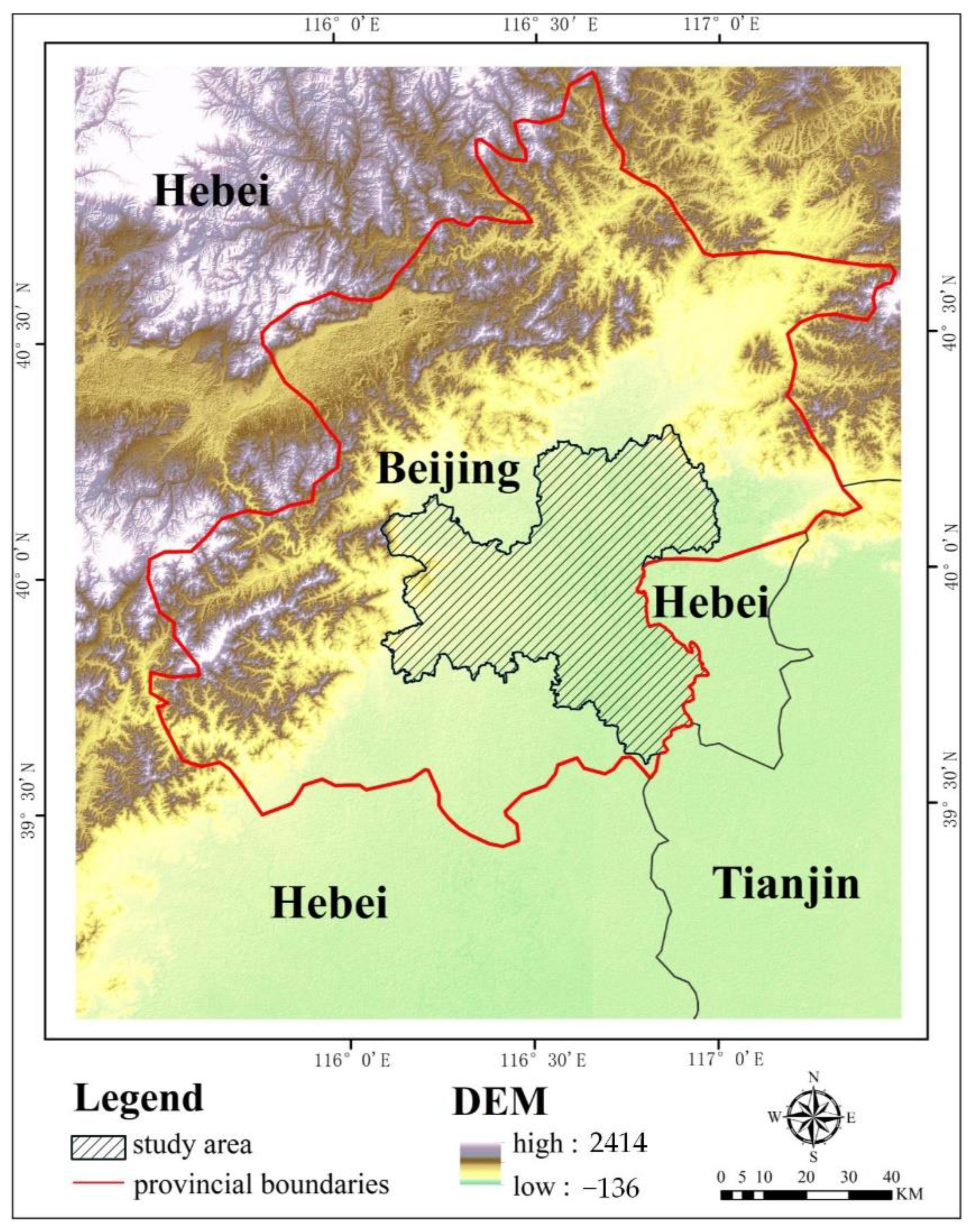
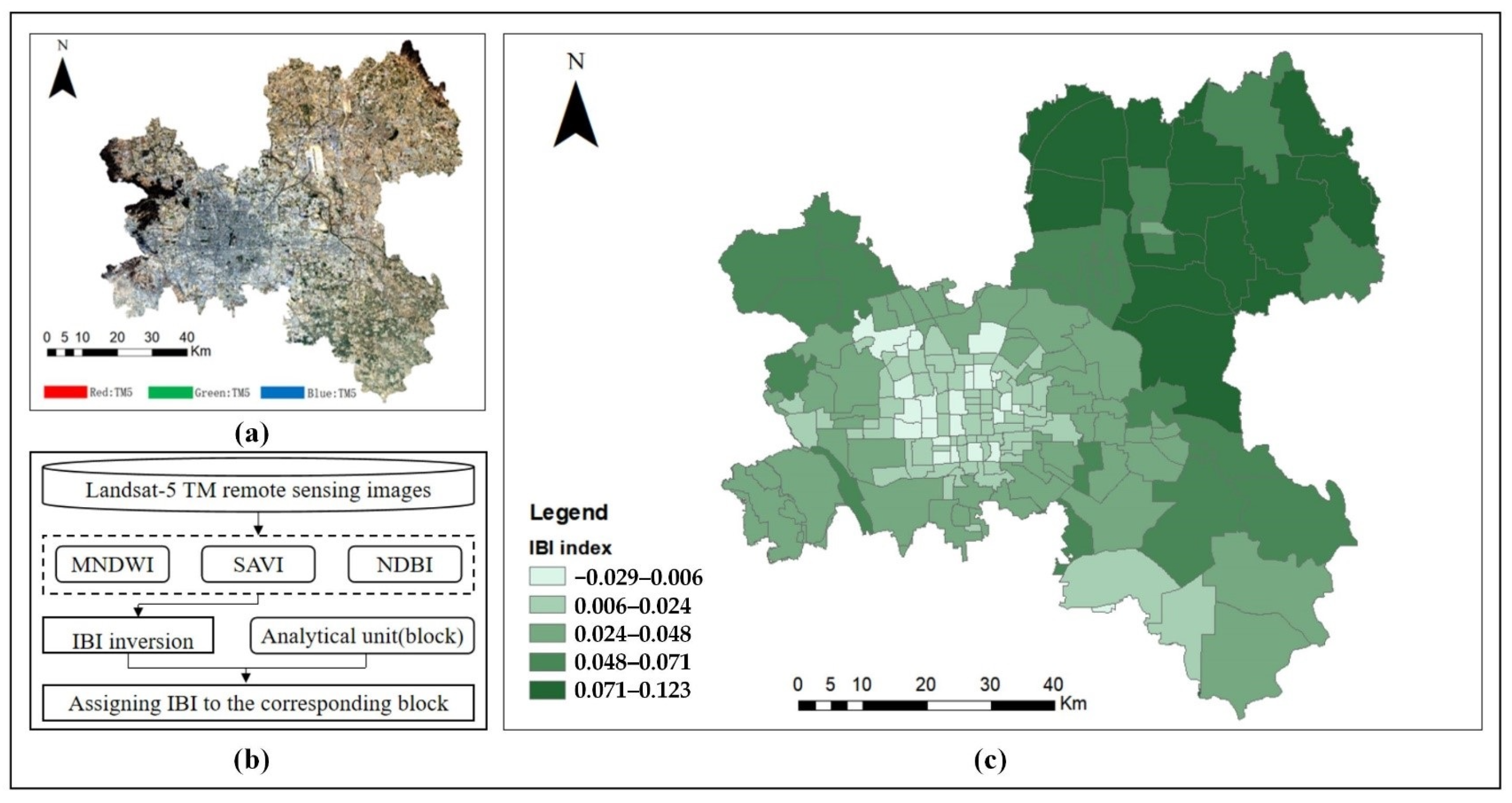
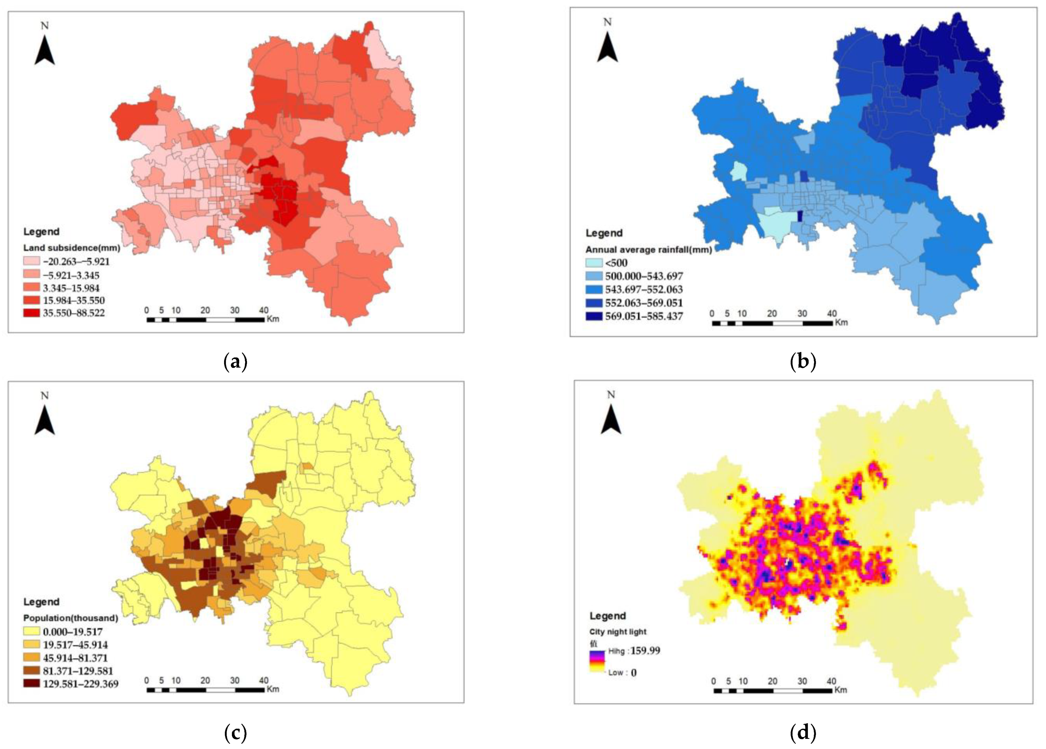
2.1. Study Area and Datasets
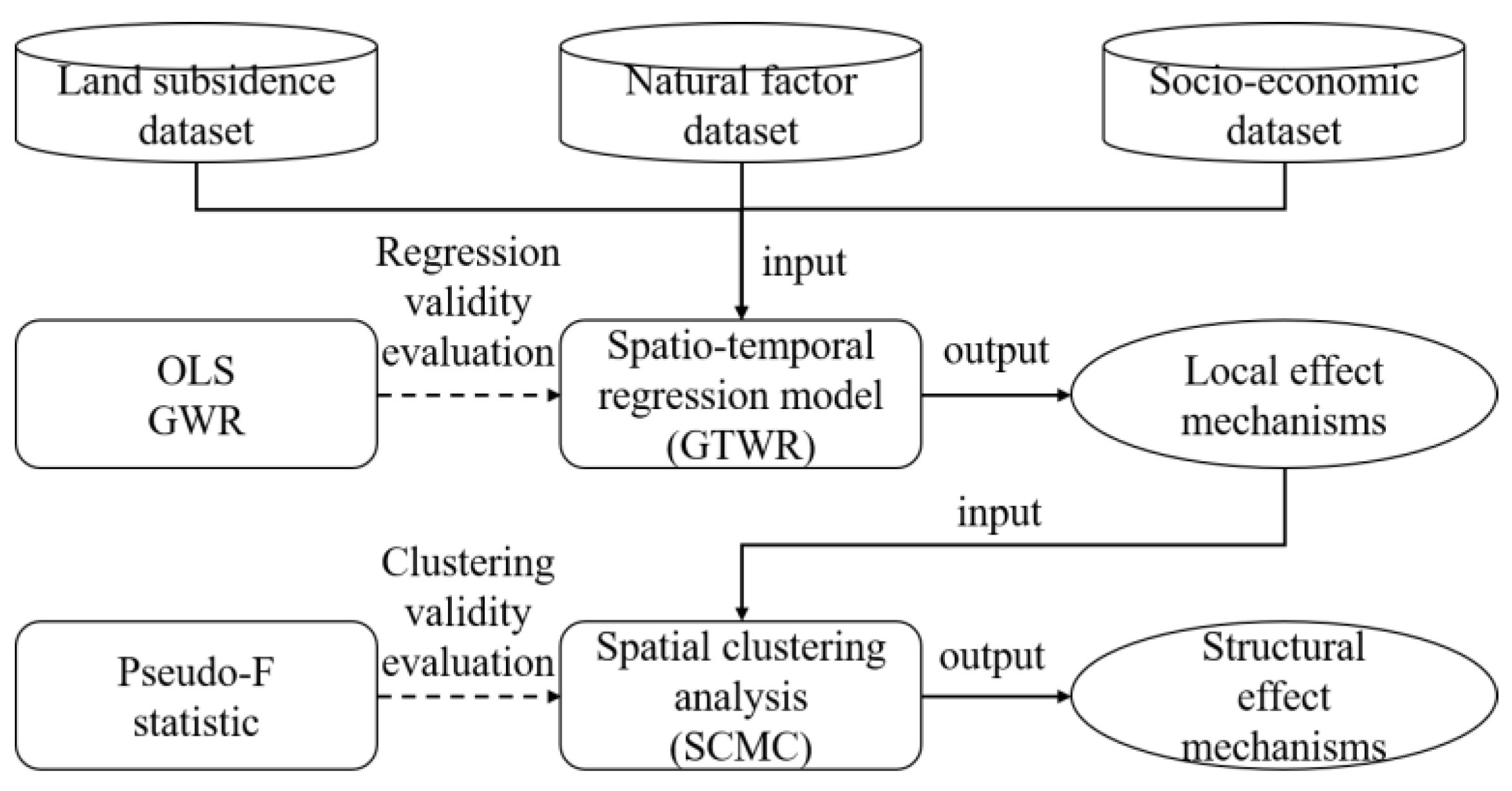
Beijing (39°26′~41°30′ N, 115°25′~117°30′ E), the capital city of China, is located on the northwestern edge of the North China Plain (see Figure 1). Eight districts under the jurisdiction of the Beijing municipality were selected as the study area, which includes the Chaoyang District, Shunyi District, Haidian District, Fengtai District, Tongzhou District, Xicheng District, Dongcheng District, and Shijingshan District, and the total area is 3303.25 km2. Following China’s reform and opening-up policy implemented in the 1980s, the process of urbanization in Beijing has significantly accelerated. Based on China’s urban statistics yearbook and data released by the National Bureau of Statistics, the central built-up area increased from 23,816 km2 in 1980 to 71,213 km2 in 1995 (expanding to the northwest of the Summer Palace, the west of Shijingshan, and the south and southeast of the Beijing Economical and Technological Development Zone) and from 83,017 km2 in 2000 to 121,012 km2 in 2005 (expanding to the Fifth Ring Road) [21]. Land subsidence in Beijing has been developing since the 1960s, and the spatial distribution is uneven, especially in Chaoyang District and Tongzhou District, where severe land subsidence has been taking place [22].
A total of 204 city blocks were selected as the basic analytical units (including town-level blocks), along with multisource datasets corresponding to those blocks (see Table 1).
The monitoring results of land subsidence in 2003–2010 were obtained by using 28 (27 + 1) synthetic aperture radar (SAR) images from the ENVISAT ASAR satellite, based on permanent scatter interferometric synthetic aperture radar (PS-InSAR). To attain the optimal overall interference effect, among the selected 27 + 1 SAR images, we selected the one with the highest overall coherence as the primary image, and the rest of the images were considered as secondary. By registering 27 auxiliary images with the main image and implementing interference processing, 27 interference pairs were obtained. The topographic phase was simulated by introducing an external digital elevation model (DEM), with a spatial resolution of 25 m and an estimated vertical accuracy of 3 m, and by performing differential interference processing, 27 interferometric phase maps could be produced. By selecting permanent scatter (PS) pixels with high coherence and using further differential interference processing, reconstructing irregular grids for those PS pixels, implementing phase unwrapping, estimating the atmospheric phase, performing multiple iterative regression analysis, and partitioning each phase and deformation phase, in the end, the deformation values of all PS pixels were obtained. In this study area, 230,028 PS pixels were identified, the density of which was about 63 pixels per km2. Level surveying data collected from the Hydrogeology and Engineering Geology Team from Beijing were used to verify the subsidence monitoring results. A total of 14 monitoring points (a total 17 points with leveling surveys and underground water level) (see Figure 2) located in the study area were selected to correspond with the PS pixels. Compared with the annual deformation of the leveling surveys and the monitoring results by PS-InSAR, the differences between the PS-InSAR monitoring results and level measurements hovered within 8 mm; consequently, the PS-InSAR measurement results were validated.
The variable (influencing factors) selection in this paper was mainly based on previous studies and depended on whether complete data collection was possible. Moreover, Xu [23] demonstrated that groundwater over-exploration was the main direct influencing factor regarding land subsidence in Beijing, and consequently, the underground water level was selected as one of the variables. The underground water level results were obtained by using the above 17 monitoring points to implement the inverse distance weighted (IDW) interpolation processing (see Figure 2). The cross validation (CV) approach was used to evaluate the interpolation accuracy, and the mean square error, standard error, and relative error were 1.75 m, 1.32 m, and 2.95%, respectively; consequently, the interpolation results were effective to meet the subsequent demand. The other variables included the average annual rainfall, block population, DMSP/OLS (1999–2012) nighttime satellite datasets, and static load. Among these, the nighttime satellite datasets were used to represent the state of economic development, and the static load information was represented by a new index-based built-up index (IBI) (see Figure 3), which was first proposed by Xu in 2008 [23]. Considering the complexity of the spectral nature of construction land, the IBI was constructed using three composited remote sensing indices: the modification of the normalized difference water index (MNDWI), the soil-adjusted vegetation index (SAVI), and the normalized difference built-up index (NDBI). Considering the dataset’s integrity, this study decided on a study period from 2003 to 2010, and the spatial distribution of all the variable values in 2006 is shown in Figure 4.

2.2. Methods

Using the spatiotemporally varying regression model, whose parameters change over space, the local effect mechanisms (the relationship between land subsidence and related natural/socioeconomic factors in each block) were obtained. The first law of geography claims that all things are related, but nearby things are more related than distant things [24], which means that the local effect mechanisms of land subsidence between adjacent blocks are more similar than that of those that are more distant. Therefore, the adjacent blocks with similar relationships between land subsidence and its associated factors are aggregated into a cluster (subarea), and the whole study area can be divided into several sub-areas. Defining similar relationships in each subarea as structural effect mechanisms and detecting them is essentially consistent with spatial clustering analysis, aiming to partition a dataset into several clusters based on attribute similarity and spatial proximity. Therefore, this method can be described as detecting structural effect mechanisms by analyzing the aggregation pattern of local effect mechanisms.
As shown in Figure 5, the methodology used in this study mainly included two steps. First, the local effect mechanisms of natural and socioeconomic factors on land subsidence were identified using geographically and temporally weighted regression (GTWR) [25]. The effectiveness of the regression results of the GTWR model was evaluated by comparison regression models, such as ordinary least-squares regression (OLS) and geographically weighted regression (GWR). Second, the structural effect mechanisms of various associated factors on land subsidence were identified by using a spatially constrained multivariate clustering (SCMC) algorithm. The optimal clustering results were determined by using the Calinski–Harabasz pseudo F-statistic [26].

2.2.1. Identifying Local Effect Mechanisms Using the GTWR Model

Spatial heterogeneity refers to the heterogeneity and complexity of spatial processes and patterns such as ecology and society in spatial distribution, which means that for a given area with spatial heterogeneity, the relationships between the dependent variables and explanatory variables are not constant, and a global model cannot demonstrate the spatial variation in the relationships among the spatial data [27]. One of the most widely used methods for achieving higher accuracy in spatial heterogeneous analysis is the GWR model [28], which enables the exploration of local effect mechanisms and the obtaining of equations of regression for each spatial area separately [29]. Despite the advantages of GWR in processing spatial variations, it is difficult to deal with dynamic geographical data with temporal heterogeneity. For dynamic geographical data, spatial–temporal heterogeneity may exist, which means the relationships among diverse variables may not only change over space, but also vary at different timestamps. Unlike the GWR model, which only takes spatial heterogeneity into account when estimating the relationships among different variables, GTWR can build a series of local models based on a weighting matrix, referencing both spatial and temporal heterogeneity [25,30].
Assuming that a land subsidence (LS) observation sample is labeled i (i = 1, 2, …, n), where n is the number of observations, the GTWR model expression is:
L S u i , v i , t i = β 0 u i , v i , t i + Σ k β k u i , v i , t X i k + ε u i , v i , t i
where L S u i , v i , t i is the land subsidence value of the monitoring site i at location u i , v i on time ti, ui, and vi are the longitude and latitude coordinates of area i, X i k represents the value of the k-th explanatory variable at sample I (k is the total number of related explanatory variables), respectively, β 0 u i , v i , t i is the space-time intercept term of location I, β k u i , v i , t i donates the slope coefficient of the kth variable of sample I, which describes the relationship between the kth variable and land subsidence, and ε u i , v i , t i represents the independent random error term. The estimation of each regression coefficient at the monitoring site I can be obtained by using the locally weighted least-square method:
β ^ u i , v i , t i = [ X T W u i , v i , t i X ] 1 X T W u i , v i , t Y
where the weight matrix W u i , v i , t i = d i a g w i , 1 , w i , 2 , , w i , n represents the diagonal matrix of the weight of spatial and temporal distance of order n. The estimated value of the weight parameter w i j depends on the spatiotemporal distance function between observation samples j and i. In general, a Gaussian distance decay-based function is used to determine the weight value:
w i j = e x p ( d i j S T ) 2 ( b S T ) 2
where the spatial–temporal d i j S T denotes a linear combination of spatial distance d i j S and temporal distance d i j T between observation samples j and I, and b S T represents the spatiotemporal bandwidth parameter used to make a decay of influence with respect to distance.
The GTWR model is determined by two types of parameters: the regression coefficient parameter and spatiotemporal bandwidth parameter. The former can be directly determined based on Equation (2), in which the weight matrix is dependent on the spatiotemporal bandwidth parameter shown in Equation (3); thus, the latter should be determined first. The regression coefficients vary depending on the spatiotemporal bandwidth parameters; thus, determining the appropriate bandwidth is key to good regression results. For the optimal selection of the bandwidth of b, generally evaluating the cross-validation (CV) function values under various bandwidth parameters, when the CV is the minimum value, the corresponding b is the optimal bandwidth [31]. All of the above work was conducted in this study using the ArcGIS 10.2 platform with the GTWR_Beta package [25].

2.2.2. Detecting Structural Effect Mechanisms Using the SCMC Algorithm

Spatial clustering, one of the research directions of cluster analysis, is an important method of spatial data mining to study the classification problem (sample or index). Although many spatial clustering algorithms have been employed to detect aggregation patterns, in this study, the SCMC algorithm was employed to spatially identify contiguous clusters of sites. By using an algorithm based on an unsupervised machine learning process, the SCMC method is used to determine the solution that maximizes both intra-cluster similarity and inter-cluster differences [32,33]. The SCMC algorithm has some parameters that can be used to represent the spatial aspect, to select the suitable variables to identify the clusters, to determine the optimum number of clusters, and to evaluate the membership probabilities. The following sections relate each of these parameters in detail.
Spatial aspect: In this study, the spatial aspect refers to using the spatial constraints parameter to represent the spatial relationships (spatial neighboring) among 204 city blocks. Because each city block is a polygon, it is appropriate to determine these spatial relationships by choosing the option of contiguity edges corners, which reflects that clusters will contain contiguous polygon features, and only polygons that share an edge or a vertex can be part of a same cluster.
Optimal number of clusters: To determine each cluster, the SCMC method first specifies a subset of seed units (city blocks with the related influencing factor data of land subsidence) randomly. Then, by computing a mean data center for each cluster of units, each unit is reassigned to the closest center. To estimate the optimal number of clusters, the Calinski–Harabasz pseudo F-statistic [26] is applied in this study, as presented by the following equations:
C H = T 2 n c 1 1 T 2 n n c
where CH is the Calinski–Harabasz pseudo F-statistic, nc is the number of clusters, n is the number of units (equal to 204), and T2 is defined as the following equations:
T 2 = S S T S S E S S T
where SST is a reference of inter-cluster differences (defined as Equation (6)), and SSE is a reference of intra-cluster similarity (defined as Equation (7)).
S S T = m = 1 n c j = 1 n i k = 1 n v v m j k v k ¯ 2
S S E = m = 1 n c j = 1 n i k = 1 n v v m j k v g k ¯ 2
where ni is the number of units in cluster m; nc is the number of clusters; nv is the number of variables used to group units; v m j k is the value of the kth variable of the jth unit in the mth cluster; v k ¯ is the mean value of the kth variable; and v g k ¯ is the mean value of the kth variable in cluster m. The pseudo F-statistic is, by default, implemented for 30 simulations (starting from 2 clusters, 3 clusters, …, resulting in 29 clusters). The highest pseudo F-statistic value among those simulations corresponds to the optimal number of clusters.
Analysis of regression coefficients of each variable to distinguish clusters: In this study, by using the GTWR approach to perform spatiotemporal regression for land subsidence (annual subsidence rate from 2003 to 2010) and the related 4 influencing factors (underground water, population, annual average rainfall, and static load), the regression coefficients of each influencing factor could be obtained, respectively. The SCMC analysis calculates the R2 value for each variable, which is more effective to divide the study area into clusters of features [32,33]. The larger the R2 value, the better discrimination among those features. In other words, the R2 value reflects how much of the variation in the coefficients of each variable was retained after the clustering process [34]. The R2 value is defined as follows:
R 2 = T S S E S S T S S
where TSS is the total sum of squares, defined by squaring and then summing deviations from the global mean value for a particular variable, and ESS is the explained sum of squares, defined the same way, except those deviations are calculated by subtracting every value from the mean value for the cluster it belongs to, and is then squared and summed.
Membership probabilities: The evaluation of membership likelihood was conducted by using 1000 permutations of random spanning trees and evidence accumulation [35]. This process was implemented using the skater approach [32,35]. The permutation process implemented by the skater method differentiates between features that switch clusters between the spanning trees that are varied and those that do not switch. Features that do not switch clusters owing to variations in the spanning tree are assigned with high membership probabilities, while features that switch clusters are assigned with low membership probabilities. The low membership probability reflects that features could be classified in a different cluster group, whereas a high membership probability indicates confidence that the feature belongs in the cluster group in which it was included. The variation range of a membership probability is from 0 to 1.

3. Results

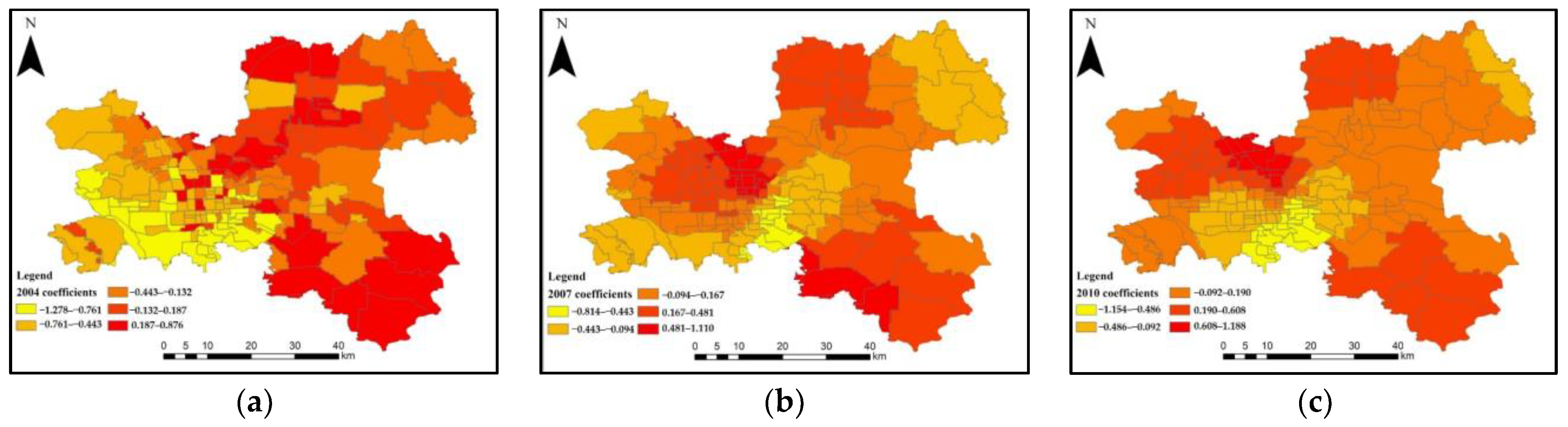
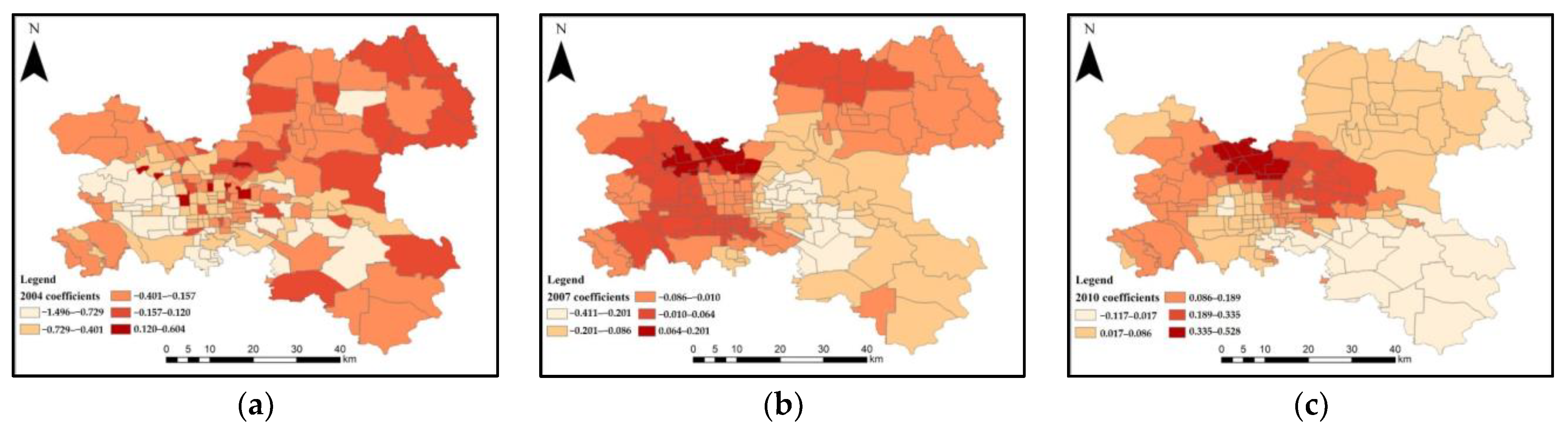
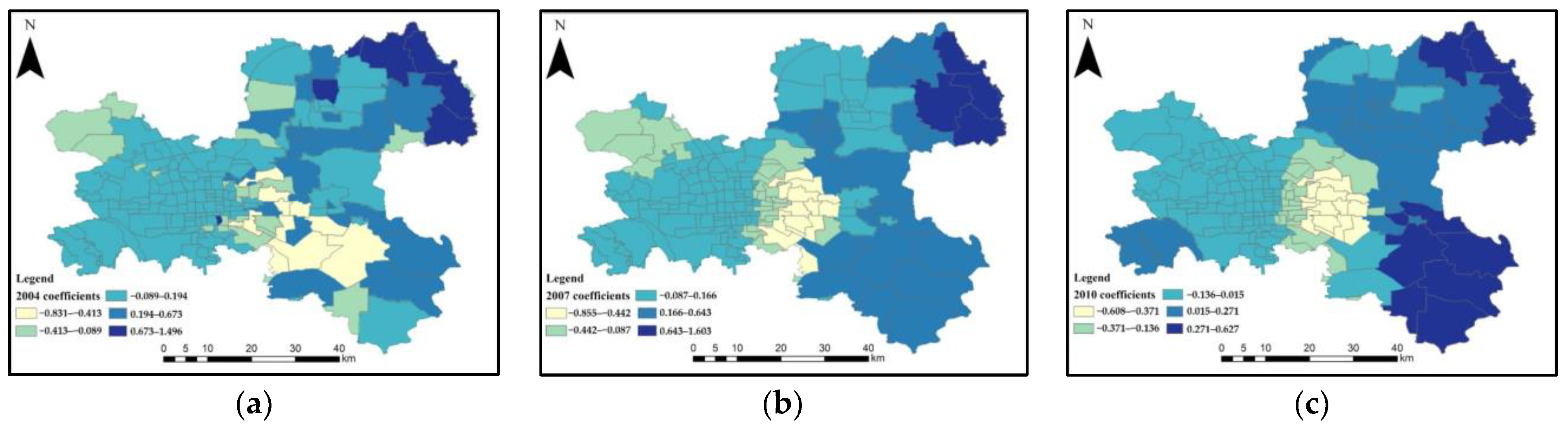
3.1. Identification of Local Effect Mechanisms of Associated Factors on Land Subsidence

In order to determine the ultimate independent variables, the variance inflation factor was employed to detect the degree of multi-collinearity, and a t-test was employed to determine the statistical significance of the regression coefficient. Four variables, namely underground water, land static load, annual average rainfall, and block population, were identified as the most closely associated with changes in land subsidence in this study region. Then, the GTWR model was used to demonstrate the spatiotemporal variation in the relationships between land subsidence and the above variables. To verify the applicability and accuracy of the GTWR model, comparing the performance results with the OLS and GWR models, four accuracy evaluation indices were used: R2, adjusted R2, AICC information, and root mean square error (RMSE) (Table 2).
R2, or adjusted R2, can reflect the degree of model fitting: the larger the value is, the higher the fitting degree will be. RMSE reflects the size of model accuracy: the smaller the value is, the higher the accuracy of the model will be, and the AICC is another important criterion to evaluate the goodness of the model fitting: the smaller the value is, the higher the accuracy of the model will be. According to Table 2, the AICC value is reduced from 12.924 of GWR and 13.952 of OLS to 12.730 of GTWR, showing that there are significant differences in performance between these models. The fitting degree (R2) of the GTWR model is 0.672, which is greatly improved compared with a GWR of 0.524 and OLS of 0.062. The further evaluation of the model performance is executed using out-of-sample validation (80% random samples for modeling and the remaining 20% for validation/prediction analysis). The RMSE value is reduced from 12.355 (GWR) and 17.344 (OLS) to 6.681 (GTWR), indicating that the prediction precision of the GTWR model is relatively higher. From the above comprehensive comparison results, the GTWR model outperforms the GWR and OLS models in describing spatiotemporal variations in land subsidence and other independent variables.
The spatial distributions of the GTWR regression coefficients for the various independent variables in 2004, 2007, and 2010 (Figure 6, Figure 7, Figure 8 and Figure 9; the given significance level is 0.05) demonstrate that they are characterized as a significant spatial aggregation trend. In other words, the estimated coefficient values at nearby locations tended to be closer. To reveal the spatial distribution of those regression coefficients in Figure 6, Figure 7, Figure 8 and Figure 9, these estimated values of the regression coefficients for all blocks are marked using several different colors in the whole study area. The minimum values of the regression coefficients of these four independent variables are negative (−1.682, −1.800, −9.720, and −0.917; Table 3), whereas the corresponding maximum values (1.188, 0.604, 14.401, and 1.734) are positive. This finding demonstrates that all variables have both negative and positive influences on land subsidence.
As shown in Table 3, according to the mean values of the regression coefficients, when the underground water level, static load (IBI), and population increased by 1 m, 1 IBI, and 10 thousand, respectively, the land subsidence increased by approximately 0.106 mm, 0.126 mm, and 0.027 mm per year, respectively, whereas when the annual average rainfall increased by 1 mm, the land subsidence decreased by 1.361 mm per year. Additionally, the coefficient of variance (CV), which is used to measure the degree of dispersion of variables with different units, is calculated by the ratio of the standard deviation (Std.) to the mean value. The order of the coefficient variation from large to small is the population, underground water, static load (IBI), and annual average rainfall.

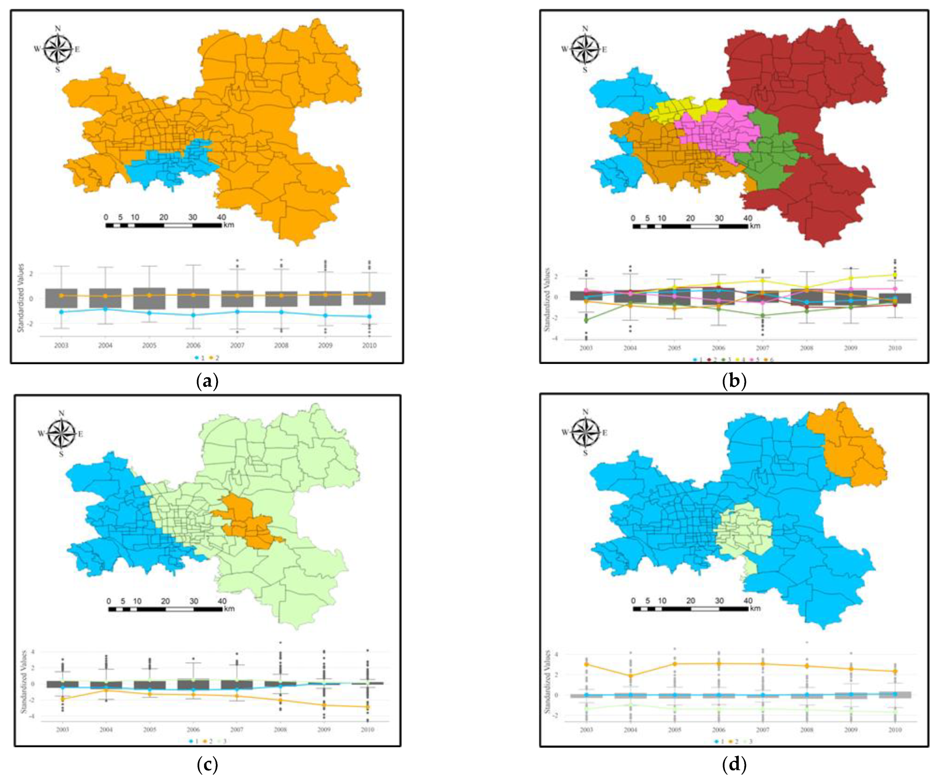
3.2. Identification of Structural Effect Mechanisms of Associated Factors on Land Subsidence

As shown in Figure 6, Figure 7, Figure 8 and Figure 9, these regression coefficients of the four variables were characterized as obvious spatial aggregation. In this study, the SCMC clustering method was used to quantitatively detect the aggregation structure for all four independent variables.

3.2.1. Estimating Number of Clusters

For each variable, the optimal number of clusters that maximized both intra-cluster similarity and inter-cluster differences (highest pseudo F-statistic value) were determined by the regression coefficients from 2003 to 2010. The analysis for underground water resulted in two clusters, the analysis for IBI resulted in six clusters, and the analyses for rainfall and population each resulted in three clusters. For most of the variables, the pseudo-F statistic value decreased strongly after the 10th simulation (simulating 10 clusters). Figure 10 shows the distribution of the pseudo-F statistic value vs. the simulations (number of clusters).

3.2.2. Regression Coefficients and Structural Characteristics

Figure 11 shows the spatial distribution of the clusters of features, including the parallel box summarizing descriptive statistics (interquartile range, median values, and outliers) for each variable (underground water, IBI, rainfall, and population). The x-axis in the parallel box plots represents the regression coefficients from 2003 to 2010, whereas the y-axis represents the standardized values. Note that each colored line for the box plots represents a different cluster group; meanwhile, the line colors also correspond to the colors displayed in the maps. For example, the underground water has two clusters: blue represented cluster 1 and orange represented cluster 2 (see Figure 11). Moreover, the variation in each line is based on the median values from coefficients per year from 2003 to 2010. For example, considering the underground water variable, Figure 11a shows that cluster 1 (blue) reflects features with low influence on land subsidence in 2004, while cluster 2 (orange) reflects features with median influence (1st quartile) on land subsidence in 2004.
As shown in Figure 11, the four variables presented different spatial distributions and box plots. For the variable of underground water (see Figure 11a), there were two clusters: cluster 1 (blue) was only a very small area located in Chaoyang District and Fengtai District; meanwhile, the two lines had similar variation trends, with small fluctuation. For the variable of IBI (see Figure 11b), there was the highest number (6) of clusters, among which cluster 2 was the biggest, covering most of the area of Shunyi District and Tongzhou District, while cluster 4 was the smallest, located in Haidian District. The six lines had different variation trends. For the variable of rainfall (see Figure 11c), there were three clusters, with cluster 1 (blue) located in the west of the study area (including Haidian District and Fengtai District), and cluster 2 (orange) being the smallest, located in Chaoyang District and Fengtai District, whereas cluster 3 (green) was the biggest, covering the majority of the study area. The green line (cluster 3) showed a horizontal change trend, which reflects that the rainfall had a steady influence on land subsidence within cluster 3 during the period, and the other two lines both showed slightly fluctuating trends. For the variable of population (see Figure 11d), cluster 2 and cluster 3 both corresponded to small regions, with the former located in the northeast of Shunyi District, and the latter in Chaoyang District. Cluster 1 covered the vast majority of the study area. From the variation in lines, the blue line (cluster 1) and green line (cluster 3) were similar, with a steady trend, while the orange line (cluster 2) had a slight fluctuating trend.
The R2 values for the four variables are shown in Table 4, and these values were listed for the regression coefficients of each variable. The larger the R2 value, the greater the difference that was identified among these features. Overall, underground water and rainfall were the variables that most effectively divided the study area into clusters of features, with an obvious spatial aggregation characteristic, while IBI and population were the variables that less effectively divided the study area into clusters of features. When the analysis was performed for the annual regression coefficients, among the four variables, the highest R2 value was for 2004.

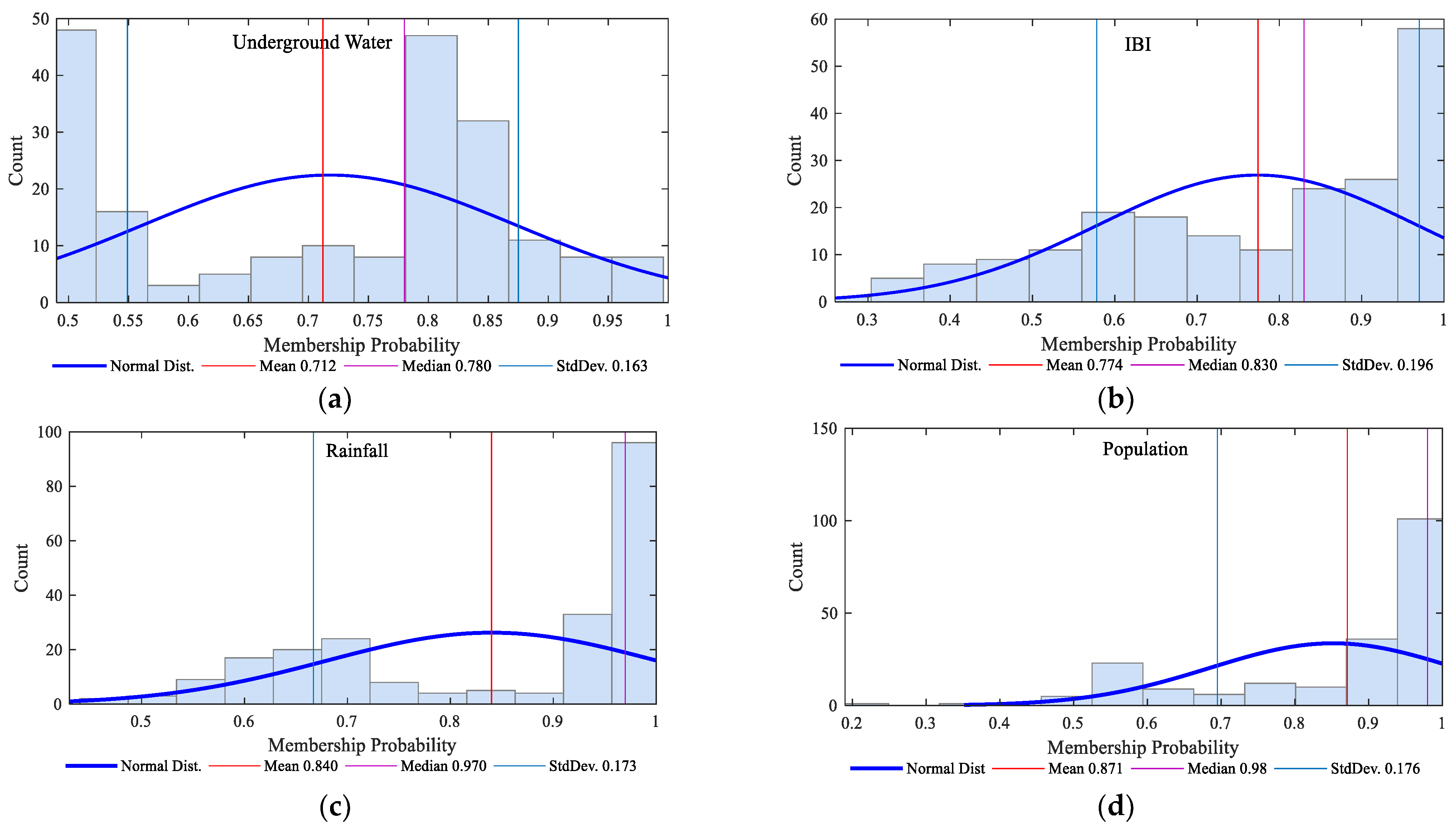
3.2.3. Cluster Membership Likelihood

Histograms (including mean and standard deviation values) of membership probability are shown in Figure 12. Those results present a confidence of likelihood of significant various conclusions (e.g., whether a particular feature should be classified into a different cluster). The higher the membership probability (highest value = 1), the higher the confidence in the results, while the lower the membership probability (lowest value = 0), the lower the confidence in the results. On the whole, these results are relatively significant in terms of confidence. From the results shown in Figure 12, overall, all results showed relatively high likelihood, with better classifications. The lowest mean membership probability value was for underground water (Mean = 0.712, StdDev = 0.163), while the highest mean probability value was for population (Mean = 0.871, StdDev = 0.176).

4. Discussion

This paper analyzed spatiotemporal variations in the effect mechanisms of associated factors on land subsidence in Beijing from 2003 to 2010. The effect mechanisms consist of local (spatiotemporal variations in each analytical unit at the individual unit/block level) and structural (aggregation patterns of multiple analytical units from the global level) models. The GTWR method was adopted to explore the local effect mechanisms by modeling the relationships between land subsidence and its influencing factors, and then, the SCMC approach was employed to detect the structural effect mechanism by dividing the study area into several quasi-homogeneous spatial subareas, according to the regression coefficient similarities. Overall, the findings reflect a substantial variation in clusters among the associated factors of land subsidence. The natural and socioeconomic variables of land subsidence showed a considerable impact on the identification of one cluster from another.
Regarding the local effect mechanisms presented by the GTWR model, all variables had both negative and positive effects on land subsidence. For example, the rainfall variable showed both maximum positive effects and maximum negative effects. Rainfall is often thought to effectively recharge groundwater and control land subsidence in cities, which means the more rainfall, the less land subsidence. However, our findings suggest that the relationships between rainfall and land subsidence are not constant over time and space. The areas exhibiting a negative effect were mainly located in Beijing suburbs, such as Shijingshan District, Tongzhou District, and Shunyi District, while areas showing a positive effect were mainly located in the downtown area. The intensity and range of negative effects exhibited significant growth after the heavy rainfall in 2008, with an underground water recharge affecting the land subsidence.
The literature has shown that land subsidence mainly resulted from the decline in the underground water level in Beijing [4]; in other words, the underground water level should have a positive influence on land subsidence—the deeper the underground water level, the worse the land subsidence. Despite an appearance of small areas with a negative effect in our findings, the underground water level had an overall positive effect on land subsidence in most of the study area, with a growing intensity and range over time, which is consistent with the results in previous research [4]. Likewise, regarding the spatiotemporal variation in the effect mechanisms of socioeconomic factors, such as population and static load, these undoubtedly induce land subsidence. Generally, owing to daily living and production activities, land subsidence is worse in more populated regions. However, owing to the spatiotemporal difference in anthropogenic urban development levels and styles, the same population density in different periods or geographic areas may result in different human activities, such as urban infrastructure construction, water consumption, and land-use change, which will have different impacts on land subsidence. For the static load (IBI) variable, our findings present an obvious changing trend from a negative effect to a positive effect over time, which means that land subsidence becomes worse with the increase in static load. The possible reason was a large amount of venue construction for the Beijing 2008 Olympic Games, with a corresponding increasing static load.
From the structural effect mechanisms presented by the SCMC method, all four variables showed substantial structural aggregation characteristics from 2003 to 2010, respectively. However, the structural effect mechanisms (including cluster number, cluster location, cluster size, and the spatiotemporal variation) were different for the four variables. The underground water variable presented two clusters. The first cluster presented the negative influence covering a small part of the areas, and the regression coefficients were found at a variation range located in the median to the 3rd quartile, while the second cluster presented the positive influence covering the vast majority of areas, and they were found under the 1st quartile. The static load (IBI) variable presented six clusters, and the other clusters were relatively balanced in size, except for cluster 2. Their regression coefficient statistic characteristics were relatively complex. The rainfall variable was composed of three clusters. Cluster 2, covering the smallest part of the areas, presented a negative influence, and its regression coefficients showed a trend of first dropping, and then rising. The regression coefficient values showed a small fluctuation trend at the 1st quartile in cluster 1, but a steady changing trend at the 3rd quartile in cluster 3. The population variable was composed of three clusters. Cluster 1 showed a very steady changing trend at the 3rd quartile (equal to 0). Cluster 2 presented a positive larger influence, and the coefficient values slightly fluctuated above 2, while cluster 3 presented a negative influence in a range of outliers.
Although the GTWR algorithm can effectively deal with the linear relationships with spatiotemporal heterogeneity, it cannot describe the possible nonlinear relationships between land subsidence and its associated factors. Therefore, it is necessary to pose a method of simultaneous nonlinearity and spatiotemporal patterns. In addition, different input variables (independent variables) result in different regression output results. In other words, the combination of variables (including quantity and quality) has a dominant influence on the output results. However, many related influencing factors (input variables) regarding land subsidence are usually hard to obtain, especially for underground water. We presented the underground water variable by using IDW interpolation based on 17 monitoring points; nevertheless, the lower density and uneven spatial distribution of these points produced interpolation results of low quality, thus affecting the regression results. Similarly, the dependent variable will also affect the regression output results. The dependent variable (land subsidence) was obtained by using PS-InSAR, which only tracks permanent scatters (PS) to obtain land deformation information, while the lack of PS pixels in limited areas will lead to a lack of deformation information [36]. Although the overall land subsidence results can be obtained by using interpolation based on PS pixels, the interpolation accuracy could be affected owing to the uneven spatial distribution of the PS pixels.
For each variable, we performed spatial clustering analysis for the regression coefficients per year using the SCMC method. In practice, clustering and the mapping of clusters could serve as a method for visual and quantitative inspection of complex datasets. If the result is appropriate, those output clusters could be used as management zones for the relevant authorities. Spatially contiguous clusters/zones resulting from applying the SCMC approach could be beneficial if technology does not allow management of individual analytical unit (city block unit) land subsidence, or if small-scale operational variations are too costly.

5. Conclusions

Land subsidence is the displacement of ground surface vertically over a broad region or in localized areas. It may be either a gradual lowering or a collapse. This can have a costly effect on facilities and structures over a subsiding area. Understanding the effect mechanisms of various factors on land subsidence may aid in the development scientific measures to control land subsidence. However, the scarcely discussed structural effect mechanisms at a small scale suggests a need to further explore their effects on land subsidence. Therefore, in this paper, an analytical framework was proposed to elaborate the structural effect mechanisms of influencing factors of land subsidence. The GTWR method was adopted to explore the local effect mechanisms by modeling the relationships between land subsidence and its influencing factors, and then the SCMC approach was employed to detect the structural effect mechanisms by dividing the study area into several quasi-homogeneous spatial subareas, according to the regression coefficient similarities.
This study expands the scientific knowledge on spatiotemporal variations in land subsidence, which can effectively provide guidance to public policymakers. Better knowledge of this relationship should be of interest to policymakers to help them develop future policies related to the prevention and control of land subsidence. Further research should include quantitatively analyzing the political functions of the land subsidence effect mechanisms.

Author Contributions

Conceptualization, B.Z., X.Y., Q.W. and M.D.; data curation, B.Z.; methodology, B.Z., X.Y. and W.X.; visualization, B.Z., W.Y. and X.Y.; writing—original draft, B.Z. and X.Y.; writing—review and editing, B.Z., X.Y., Q.W. and M.D. All authors have read and agreed to the published version of the manuscript.

Funding

This research was supported by grants from the National Natural Science Foundation of China (41901319, 41730105, and 42171459), the Natural Science Foundation of Hunan Province (2022JJ40585), and the Independent Exploration and Innovation Project Fund Designated for Graduate Students of Central South University (2018zzts205).

Institutional Review Board Statement

Not applicable.

Informed Consent Statement

Not applicable.

Data Availability Statement

Not applicable.

Acknowledgments

This work was carried out, in part, using computing resources at the High-Performance Computing Platform of Central South University.

Conflicts of Interest

The authors declare no conflict of interest.

References

  1. Galloway, D.L.; Burbey, T.J. Review: Regional land subsidence accompanying groundwater extraction. Hydrogeol. J. 2011, 19, 1459–1486. [Google Scholar] [CrossRef]
  2. Herrera-García, G.; Ezquerro, P.; Tomás, R.; Béjar-Pizarro, M.; López-Vinielles, J.; Rossi, M.; Mateors, R.M.; Carreón-Freyre, D.; Lambert, J.; Teatini, P.; et al. Mapping the global threat of land subsidence. Science 2021, 371, 34–36. [Google Scholar] [CrossRef] [PubMed]
  3. Anonymous. Land Subsidence International Symposium Held in VENICE; Eos Transactions American Geophysical Union: Hoboken, NJ, USA, 1984; Volume 65, p. 1180. [Google Scholar]
  4. Si, Y.; Chen, B.B.; Gong, H.L.; Gao, M.L. Temporal and spatial evolution of land subsidence induced by groundwater exploitation and construction in the eastern Chaoyang district, Beijing, China. J. Indian Soc. Remote Sens. 2018, 46, 1657–1665. [Google Scholar] [CrossRef]
  5. Chaussard, E.; Wdowinski, S.; Cabral-Cano, E.; Amelung, F. Land subsidence in central Mexico detected by ALOS InSAR time-series. Remote Sens. Environ. 2014, 140, 94–106. [Google Scholar] [CrossRef]
  6. Conway, B.D. Land subsidence and earth fissures in south-central and southern Arizona, USA. Hydrogeol. J. 2016, 24, 649–655. [Google Scholar] [CrossRef]
  7. Bhattarai, R.; Kondoh, A. Risk assessment of land subsidence in Kathmandu valley, Nepal, using remote sensing and GIS. Adv. Remote Sens. 2017, 6, 132–146. [Google Scholar] [CrossRef]
  8. Rahmati, O.; Golkarian, A.; Biggs, T.; Mohammadi, F.; Daliakopoulos, I.N. Land subsidence hazard modeling: Machine learning to identify predictors and the role of human activities. J. Environ. Manag. 2019, 236, 466–480. [Google Scholar] [CrossRef]
  9. Luo, Z.J.; Zeng, F. Finite element numerical simulation of land subsidence and groundwater exploitation based on visco-elasticplastic biot’s consolidation theory. J. Hydrodyn. 2011, 23, 615–624. [Google Scholar] [CrossRef]
  10. Zhou, Y.X.; Li, W.P. A review of regional groundwater flow modeling. Geosci. Front. 2011, 2, 205–214. [Google Scholar] [CrossRef]
  11. Tsangaratos, P.; Ilia, I.; Loupasakis, C. Land subsidence modelling using data mining techniques. The case study of western Thessaly, Greece. In Advances in Natural and Technological Hazards Research; Pourghasemi, H.R., Rossi, M., Eds.; Springer International Publishing: Berlin/Heidelberg, Germany, 2018; pp. 79–103. [Google Scholar]
  12. Pourghasemi, H.R.; Mohseni Saravi, M. Land-subsidence spatial modeling using the random forest data-mining technique. In Spatial Modeling in GIS and R for Earth and Environmental Sciences; Pourghasemi, H.R., Gokceoglu, C., Eds.; Elsevier: Amsterdam, The Netherlands, 2019; pp. 147–159. [Google Scholar]
  13. Wang, J.F.; Xu, C.D. Geodetector: Principle and prospective. Acta Geogr. Sin. 2017, 72, 116–134. [Google Scholar]
  14. Hu, K.; Wei, L.; Liu, S.; Li, X.Z. Spatial pattern of debris-flow catchments and the rainfall amount of triggering debris flows in the Hengduan Mountains region. Acta Geogr. Sin. 2019, 74, 2303–2313. [Google Scholar]
  15. Yang, H.O.; Chen, W.B.; Liang, Z.F. Impact of land use on PM2.5 pollution in a representative city of middle China. Int. J. Environ. Res. Public Health. 2017, 14, 462. [Google Scholar] [CrossRef] [PubMed]
  16. Xiao, W.F.; Yang, W.T.; Li, C.K.; Tian, H.B.; Zheng, D.Y.; Bo, P. Detection of influence factors and their interaction of land subsidence in Beijing based on PS-InSAR. Geomat. World 2020, 27, 7–13. [Google Scholar]
  17. Jiang, D.C.; Zhang, J.X.; Zhang, Y.H.; Wu, H.A.; Kang, Y.H. Ground deformation over century-long coal mining city monitored through incorporating both PS and SBAS InSAR: A case study of Xuzhou. Bull. Surv. Mapp. 2017, 1, 58–64. [Google Scholar]
  18. Minderhoud, P.S.J.; Coumou, L.; Erban, L.E.; Middelkoop, H.; Stouthamer, E.; Addink, E.A. The relation between land use and subsidence in the Vietnamese Mekong delta. Sci Total Environ. 2018, 634, 715–726. [Google Scholar] [CrossRef] [PubMed]
  19. Lu, Y.Y. Land subsidence monitoring and analysis of influencing factors in Su-Xi-Chang area based on multi-source SAR data. Acta Geod. Cartogr. Sin. 2019, 48, 938. [Google Scholar]
  20. Wang, J.F.; Zhang, T.L.; Fu, B.J. A measure of spatial stratified heterogeneity. Ecol. Indic. 2016, 67, 250–256. [Google Scholar] [CrossRef]
  21. Liu, Y.S.; Yang, Y.Y.; Li, Y.R.; Li, J.T. Conversion from rural settlements and arable land under rapid urbanization in Beijing during 1985–2010. J. Rural Stud. 2017, 51, 141–150. [Google Scholar] [CrossRef]
  22. Gong, H.L.; Pan, Y.; Zheng, L.Q.; Li, X.J.; Zhu, L.; Zhang, C.; Huang, Z.Y.; Li, Z.P.; Wang, H.G.; Zhou, C.F. Long-term groundwater storage changes and land subsidence development in the North China Plain (1971–2015). Hydrogeol. J. 2018, 26, 1417–1427. [Google Scholar] [CrossRef]
  23. Xu, H. A new index for delineating built-up land features in satellite imagery. Int. J. Remote Sens. 2008, 29, 4269–4276. [Google Scholar] [CrossRef]
  24. Tobler, W.R. A computer movie simulating urban growth in the Detroit region. Econ. Geogr. 1970, 46, 234. [Google Scholar] [CrossRef]
  25. Huang, B.; Wu, B.; Barry, M. Geographically and temporally weighted regression for modeling spatio-temporal variation in house prices. Int. J. Geogr. Inf. Sci. 2010, 24, 383–401. [Google Scholar] [CrossRef]
  26. Calinski, T.; Harabasz, J. A dendrite method for cluster analysis. In Communications in Statistics-Theory and Methods; Taylor & Francis: Abingdon, UK, 1974; Volume 3, pp. 1–27. [Google Scholar]
  27. Deng, M.; Yang, W.T.; Liu, Q.L. Geographically weighted extreme learning machine: A method for space-time prediction. Geogr. Anal. 2017, 49, 433–450. [Google Scholar] [CrossRef]
  28. Wheeler, D.C. Geographically weighted regression. In Handbook of Regional Science; Springer: Berlin/Heidelberg, Germany, 2013; pp. 1435–1459. [Google Scholar]
  29. Chalkias, C.; Kalogirou, S.; Ferentinou, M. Landslide susceptibility, Peloponnese Peninsula in South Greece. J. Maps 2014, 10, 211–222. [Google Scholar] [CrossRef]
  30. Yang, W.T.; He, Z.J.; Huang, H.K.; Huang, J.C. A clustering framework to reveal the structural effect mechanisms of natural and social factors on PM2.5 concentrations in China. Sustainability 2021, 13, 1428. [Google Scholar] [CrossRef]
  31. Brunsdon, C.; Fotheringham, A.S.; Charlton, M.E. Geographically weighted regression: A method for exploring spatial nonstationarity. Geogr. Anal. 1996, 28, 281–298. [Google Scholar] [CrossRef]
  32. AssunÇão, R.M.; Neves, M.C.; Câmara, G.; Da Costa Freitas, C. Efficient regionalization techniques for socio-economic geographical units using minimum spanning trees. Int. J. Geogr. Inf. Sci. 2006, 20, 797–811. [Google Scholar] [CrossRef]
  33. Duque, J.C.; Ramos, R.; Suriñach, J. Supervised regionalization methods: A survey. Int. Reg. Sci. Rev. 2007, 30, 195–220. [Google Scholar] [CrossRef]
  34. Requia, W.J.; Coull, B.A.; Koutrakis, P. Multivariate spatial patterns of ambient PM2.5 elemental concentrations in eastern Massachusetts. Environ. Pollut. 2019, 252, 1942–1952. [Google Scholar] [CrossRef]
  35. Lage, J.P.; Assunção, R.M.; Reis, E.A. A minimal spanning tree algorithm applied to spatial cluster analysis. Electron. Notes Discret. Math. 2001, 7, 162–165. [Google Scholar] [CrossRef]
  36. Van der Horst, T.; Rutten, M.M.; van de Giesen, N.C.; Hanssen, R.F. Monitoring land subsidence in Yangon, Myanmar using Sentinel-1 persistent scatterer interferometry and assessment of driving mechanisms. Remote Sens. Environ. 2018, 217, 101–110. [Google Scholar] [CrossRef]
Figure 1. Geographic position of the study area.
Sustainability 14 10139 g001
Figure 2. Spatial distribution of monitoring points and interpolation results of underground water levels in 2005.
Sustainability 14 10139 g002
Figure 3. Methodological flowchart and results of IBI (static load) extraction using the Landsat TM5 image: (a) Landsat TM5 satellite image in 2006, (b) flowchart of extracting IBI index (static load), (c) results of extracting IBI index (static load) of Beijing in 2006 by Landset TM5 satellite image.
Sustainability 14 10139 g003
Figure 4. Spatial distribution of all variable values (except IBI and underground water level) in 2006: (a) land subsidence, (b) annual average rainfall, (c) population, and (d) nighttime light.
Sustainability 14 10139 g004
Figure 5. Methodology of research used in this study.
Sustainability 14 10139 g005
Figure 6. Spatial distribution of the regression coefficient for the underground water level in: (a) 2004 (p-values = 0.0032), (b) 2007 (p-values = 0.0025), and (c) 2010 (p-values = 0.0041).
Sustainability 14 10139 g006
Figure 7. Spatial distribution of the regression coefficient for the static load (IBI) in: (a) 2004 (p-values = 0.0022), (b) 2007 (p-values = 0.0017), and (c) 2010 (p-values = 0.0008).
Sustainability 14 10139 g007
Figure 8. Spatial distribution of the regression coefficient for the annual average rainfall in: (a) 2004 (p-values = 0.0012), (b) 2007 (p-values = 0.0020), and (c) 2010 (p-values = 0.0032).
Sustainability 14 10139 g008
Figure 9. Spatial distribution of the regression coefficient for the population in: (a) 2004 (p-values = 0.0142), (b) 2007 (p-values = 0.0233), and (c) 2010 (p-values = 0.0086).
Sustainability 14 10139 g009
Figure 10. Pseudo-F statistic (optimal number of clusters) for (a) underground water, (b) IBI, (c) rainfall, and (d) population.
Sustainability 14 10139 g010
Figure 11. Spatial distribution of clusters and parallel box plots showing a summary of the analysis (interquartile range, median values, and outliers from each variable regression coefficients) for underground water (a), IBI (b), rainfall (c), and population (d). Note: the lines across box plots represent each cluster determined in our analysis; the variation in these lines is based on the median values from each variable; the color from each line is in agreement with the colors displayed in the maps (each color represents one cluster group).
Sustainability 14 10139 g011
Figure 12. Distribution of membership probability for (a) underground water, (b) IBI, (c) rainfall, and (d) population.
Sustainability 14 10139 g012
Table 1. Multisource datasets used in this study.
CategoryYearSpatial ScaleSource
Annual average subsidence rate2003–201030 mhttps://earth.esa.int/
(accessed on 8 December 2021)
Nighttime satellite images2003–20101 kmhttp://earthdata.nasa.gov/
(accessed on 8 December 2021)
Land static load2003–201030 mhttp://www.gscloud.cn/
(accessed on 8 December 2021)
Annual average rainfall2003–2010204 blocks (Beijing)http://www.cma.gov.cn/
(accessed on 8 December 2021)
Block population2003–2010204 blocks (Beijing)https://www.worldpop.org/
(accessed on 8 December 2021)
Underground water 2003–2010204 blocks (Beijing)http://www.cigem.cgs.gov.cn/
(accessedon 8 December 2021)
Table 2. Accuracy evaluation results for different regression models.
IndexGTWRGWROLS
AICC12,73012,92413,952
R20.6720.5240.062
Adjusted R20.6710.523-
RMSE6.68112.35517.344
Table 3. Descriptive statistics of regression coefficients for different variables.
VariableDescriptive Statistics of Regression Coefficients
MinMaxMeanStd.CV
Underground water level (m)−1.6821.1880.1060.4864.585
Static load (IBI)−1.8000.6040.1260.3092.452
Annual average rainfall (mm)−9.72014.401−1.3613.089−2.270
Population (10 thousand)−0.9171.7340.0270.32211.926
Table 4. R2 values (the effectiveness of each variable coefficient to divide the features into clusters).
Variable20032004200520062007200820092010
Underground water0.7540.8470.7140.6260.7620.7500.6100.563
IBI0.4400.6700.3350.2920.4810.3250.3010.364
Rainfall0.6350.8430.5990.5500.5610.6740.6010.539
Population0.2740.7270.2550.2480.2610.3020.3300.360
Publisher’s Note: MDPI stays neutral with regard to jurisdictional claims in published maps and institutional affiliations.

