Spatiotemporal Coupling Effect of Regional Economic Development and De-Carbonisation of Energy Use in China: Empirical Analysis Based on Panel and Spatial Durbin Models

Abstract

The synergistic development of economic construction and low-carbon transformation of energy systems must be promoted for building a green, low-carbon, and cyclic economic system and achieving the “double carbon” goal in China. Based on the panel data of 30 provincial-level administrative regions in China from 2015 to 2019, the global entropy method, coupling coordination degree model, and spatial statistical analysis methods are applied to analyse the factors affecting the coupling effect. The coordination degree increased in the study period, with Beijing, Shanghai, Tianjin, Jiangsu, and Zhejiang being the regions with the highest values. The spatial distribution of the coupling coordination degree is strongly positively correlated with the eastern provincial-level administrative regions located in the high–high concentration area of the Moran scatterplot and western provincial-level administrative regions concentrated in the low–low concentration area. The spatial association pattern is stable in the study period, with only two provinces exhibiting a transition: Shandong province made the transition to high–high agglomeration areas, and Liaoning province made the transition to low–low agglomeration areas. The level of regional economy, urbanization process, energy consumption structure, and level of investment in science and innovation enhance the coupling coordination degree, whereas the industrial structure deteriorates this degree.

1. Introduction

In the new development stage, China is committed to building a green, low-carbon, and circular economic system. Owing to environmental constraints, the energy use structures must be modified. To achieve the ‘double carbon’ goal, the relationship between the double control of energy and economic development must be managed to promote the synergistic development of economic construction and de-carbonisation of energy use. In December 2021, the Ministry of Industry and Information Technology issued the “14th Five-Year Plan for Green Development of Industry”, which recommended the acceleration of the transformation of de-carbonisation of energy use, increase in the energy use, and increase in the proportion of clean energy consumption. Moreover, this plan reiterated the specific goals of carbon emission reduction and energy intensity reduction. Notably, changing the energy structure is a gradual process, and China has been actively promoting the transformation of the energy strategy and green low-carbon economic development in recent years. Since 2014, China’s energy strategy has entered a period of accelerated transformation, and the economic development and low-carbonisation processes have yielded promising results. However, considerable differences remain in the economic scale, industrial structure, energy structure, and energy consumption in different regions, and the imbalance between the regional economic development and low-carbon energy consumption has emerged as a major problem. To study the level of coupled and coordinated development of regional economic development and low-carbonisation of energy consumption in China, the period of 2015–2019 is considered in this study, as China’s energy low-carbonisation transition entered a new phase of accelerated development after 2014.

Recently, considerable research has been conducted on the relationship between the economy, energy, and environment. The key research issues include the dynamic relationship between the energy consumption and economic growth [1,2,3,4,5] and coupled and coordinated development of energy, economy, and environment systems [6,7]. Research on low-carbonisation of energy consumption has been focused on evaluating the development of energy low-carbonisation and the development path [8,9,10,11]. However, research on evaluating the regional energy consumption differences from the perspective of low-carbon development is limited, and only a few researchers have examined the evolution characteristics of the coordinated development of the regional economy and low-carbonisation of energy consumption from the spatial and temporal dimensions.

Considering China’s basic economic and energy conditions and goals of green and low-carbon development of energy, in this study, the panel data of 30 provincial-level administrative regions from 2015–2019 are selected. The global entropy value method is used to construct a three-dimensional time-series evaluation data system of indicators for the regional economic development and low-carbonisation of energy consumption in the spatial and temporal domains. This system is used to objectively assign weights and scores to the evaluation indicators. Moreover, the coupling coordination degree model and spatial econometric analysis methods are applied to explore the coordination degree, spatial variability characteristics, and driving factors of the coupling in 30 provincial-level administrative regions in China from the spatial and temporal dimensions. Based on the research design, this paper aims to measure and analyse the spatiotemporal difference and relevance between the coordinated development of China’s regional economy and the de-carbonisation of energy use over recent years, to identify the regions with low levels of coupling coordination and with relatively unbalanced development that need to be given priority. On this basis, from the perspective of the influencing factors, further study is conducted to analyse the driving factors affecting the coupling coordination, aiming to propose targeted policies for improving the level of coordinated development, and provide the theoretical and practical reference for the construction of green, low carbon, and circular economic system in China.

2. Indicator System Construction

The connotations and coupling mechanisms of economic development and energy consumption are considered along with China’s economic and energy situation. Moreover, under the guiding principles of scientificity, systematisation, typicality, consistency, and quantifiability, the existing research results [6,7,8,9,10,11,12,13,14] are examined and experts and scholars in relevant fields are consulted to identify the key indicators that can reflect objective reality, for which adequate data are available. Seven indicators are selected from the three dimensions of economic aggregation and structure, economic efficiency, and economic and social development to build a comprehensive evaluation index system of the regional economic development level. Moreover, seven indicators are selected from the three dimensions of energy consumption, energy structure, and carbon emission scale to build a comprehensive evaluation index system of the regional low-carbonisation of the energy use level, as indicated in

Table 1. Evaluation indicators for the regional economic development and low-carbonisation of energy consumption.

Coupled Evaluation Systems	Evaluation Dimensions	Indicator	Indicator Direction	Unit
Regional economic development	Economic aggregation and structure	GDP per capita	Positive	yuan
		Proportion of added value of tertiary industry in GDP	Positive	%
	Economic efficiency	Financial revenue per capita	Positive	yuan
		Disposable income of urban residents per capita	Positive	yuan
	Economic and social development	Urbanisation rate	Positive	%
		Total retail sales of social consumer goods per capita	Positive	yuan
		Total investment in fixed assets per capita	Positive	yuan
Regional low-carbonisation of energy consumption	Energy consumption	Increase or decrease in the energy consumption per 10,000 yuan of GDP	Negative	(±%)
		Growth rate of total energy consumption	Negative	%
		Increase or decrease in the electricity consumption per 10,000 yuan of GDP	Negative	(±%)
	Energy structure	Proportion of coal consumption in energy consumption	Negative	%
		Proportion of electric energy in energy consumption	Positive	%
	Scale of carbon emissions	carbon emissions per capita	Negative	tons
		Carbon emissions per 10,000 yuan of GDP	Negative	tons/10,000 yuan

. The data for the evaluation indicators are extracted from the statistical data of the “China Statistical Yearbook”, “Statistical yearbook of China’s Fixed Assets Investment (China’s investment field)”, “China Energy Statistical Yearbook”, “China census yearbook”, and “Carbon Emission Account&Datasets” [15,16,17,18,19]. At present, with increasingly comprehensive and profound data applications, more caution should be given to data applications. Therefore, the pervasive discussion of data uncertainty is crucial in academic study, especially in economics. With thorough discussion and analysis, the raw data involved in this paper is relatively certain and stable. The main indicators involved in the study of the spatiotemporal Coupling Effect in this paper are macro indicators of regional economy and energy. Against the background of the stable macro-environment and the smooth national economic development trend, the raw data is characterized by high stability, whose change trend is regular and predictable to a certain extent, with the relatively controllable fluctuation range and the low risk of data uncertainty due to random factors. In addition, sourced from national statistical departments and relevant official institutions, raw data has a relatively high degree of reliability, accuracy and authority. It is worth noting that there are inevitable statistical errors caused by human, technical, or other factors in the process of official data. However, in recent years, with the continuous improvement of the data accounting system and strengthening of data verification and accounting by the statistical departments and relevant institutions, the error of index data has been kept within the permissible range, capable of reflecting the economic situation more objectively. Even more, these statistics are widely used in academic research, and help to obtain a large number of research results.

3. Research Methodology

3.1. Global Entropy Method

The global entropy method is an improved weighting method for the traditional entropy method, which is used to solve the objective weighting problem of three-dimensional time-series data by introducing the global concept to analyse each evaluation index horizontally and vertically in the evaluation system. Scholars in China have applied the global entropy method in different research fields to conduct multidimensional dynamic comparative analyses. Ruifen et al. [20] applied the global entropy method to conduct a dynamic comparative analysis of the regional innovation capacity of Beijing, Tianjin, and Hebei. Yusen et al. [21] applied the global entropy method to conduct a dynamic analysis and evaluation of the level of intellectual property resources in 31 provincial-level administrative regions in China. Yangjie et al. [22] applied the global entropy method to dynamically measure and analyse the industrial ecological level in the upper reaches of the Yangtze River in China.

This study is aimed at performing a dynamic evaluation of China’s regional economic development level and low-carbonisation of energy consumption level from the time and space dimensions. A three-dimensional time-series data table of time–space indices is constructed, and the global entropy method is used to objectively assign weights to the evaluation indicators. The global entropy weighting method involves the following steps [20,21]:

• Construct the initial global evaluation matrix. Considering m provincial-level administrative regions, n evaluation indicators, and T years, the global idea is introduced to arrange the data in chronological order to form a global evaluation matrix $\mathrm{A}$.

  $$\mathrm{A} = {\left({\mathrm{X}}^1,{ \mathrm{X}}^2, \cdots {\mathrm{X}}^{\mathrm{t}}\right)}_{\mathrm{m} \times \mathrm{n}}^{\prime } = {({\mathrm{x}}_{\mathrm{ij}}^{\mathrm{t}})}_{\mathrm{m} \times \mathrm{n}},$$

  (1)

  where ${\mathrm{x}}_{\mathrm{ij}}^{\mathrm{t}}$ denotes the j-th index data of the ith province in the t-th year.
• Standardise the indicator data. To eliminate the influence of inconsistencies in the evaluation indexes in terms of scale, order of magnitude, and units, the difference (Min-max) standardisation method is used to process the original data. The direction of positive indicators is consistent with the level of regional economic development and low-carbonisation of energy consumption in China evaluated in this study. That is, the larger the value, the better, while the direction of negative indicators is the opposite, and the smaller the value, the better.

  $$\mathrm{Positive} \mathrm{indicators}:{{\mathrm{x}}_{\mathrm{ij}}^{\mathrm{t}}}^{\prime } = \frac{{\mathrm{x}}_{\mathrm{ij}}^{\mathrm{t}} - {\mathrm{x}}_{\mathrm{jmin}}}{{\mathrm{x}}_{\mathrm{jmax}} - {\mathrm{x}}_{\mathrm{jmin}}},$$

  (2)

  $$\mathrm{Negative} \mathrm{indicators}:{{\mathrm{x}}_{\mathrm{ij}}^{\mathrm{t}}}^{\prime } = \frac{{\mathrm{x}}_{\mathrm{ij}}^{\mathrm{t}} - {\mathrm{x}}_{\mathrm{jmin}}}{{\mathrm{x}}_{\mathrm{jmax}} - {\mathrm{x}}_{\mathrm{jmin}}},$$

  (3)

  where $\mathrm{i} = 1, 2,\cdots ,\mathrm{m}; \mathrm{j} = 1, 2,\cdots ,\mathrm{n}; \mathrm{t} = 1, 2,\cdots ,\mathrm{T}.$
• Calculate the characteristic proportion of the i-th evaluation object under the j-th evaluation indicator in the t-th year for evaluation indicator ${\mathrm{p}}_{\mathrm{ij}}^{\mathrm{t}}$:

  $${\mathrm{p}}_{\mathrm{ij}}^{\mathrm{t}} = \frac{{{\mathrm{x}}_{\mathrm{ij}}^{\mathrm{t}}}^{\prime }}{{\sum }_{\mathrm{t} = 1}^{\mathrm{T}}{\sum }_{\mathrm{i} = 1}^{\mathrm{m}}{{\mathrm{x}}_{\mathrm{ij}}^{\mathrm{t}}}^{\prime }}.$$

  (4)
• Calculate the information entropy value of each indicator ${\mathrm{e}}_{\mathrm{j}}$:

  $${\mathrm{e}}_{\mathrm{j}} = -\frac{1}{\mathrm{lnmT}}{\sum }_{\mathrm{t} = 1}^{\mathrm{T}}{\sum }_{\mathrm{j} = 1}^{\mathrm{n}}{\mathrm{p}}_{\mathrm{ij}}^{\mathrm{t}}{\mathrm{lnp}}_{\mathrm{ij}}^{\mathrm{t}},\left(0\le {\mathrm{e}}_{\mathrm{j}}\le 1\right).$$

  (5)
• Calculate the coefficient of variation of each evaluation indicator ${\mathrm{g}}_{\mathrm{j}}$. A lower entropy of an evaluation indicator corresponds to a higher coefficient of variation and higher weight of that indicator. Define the variability factor vector $\mathrm{G} = \left({\mathrm{g}}_1,{ \mathrm{g}}_2, \cdots {\mathrm{g}}_{\mathrm{n}}\right)$.

  $${\mathrm{g}}_{\mathrm{j}} = 1 - {\mathrm{e}}_{\mathrm{j}}.$$

  (6)
• Calculate the evaluation indicator weights ${ \mathsf{\omega }}_{\mathrm{j}}$:

  $${\mathsf{\omega }}_{\mathrm{j}} = \frac{{\mathrm{g}}_{\mathrm{j}}}{{\sum }_{\mathrm{j} = 1}^{\mathrm{n}}{\mathrm{g}}_{\mathrm{j}}}.$$

  (7)
• Calculate the overall evaluation score ${\mathrm{F}}_{\mathrm{i}}^{\mathrm{t}}$:

  $${\mathrm{F}}_{\mathrm{i}}^{\mathrm{t}} = {\sum }_{\mathrm{j} = 1}^{\mathrm{n}}{\mathsf{\omega }}_{\mathrm{j}}{{\mathrm{x}}_{\mathrm{ij}}^{\mathrm{t}}}^{\prime }.$$

  (8)

3.2. Coupling Coordination Model

The term ‘coupling’ refers to a physics concept indicating the close correlation between the input and output of circuit elements and is widely used at present in various research fields to reflect the interrelationship between systems or between elements in systems. With the development of multidisciplinary integration, the coupling research theory has yielded notable results in regional development. Xin et al. [23] applied the coupling coordination degree model to study the spatiotemporal coupling relationship between new urbanisation and low-carbonisation of development in 30 provincial-level administrative regions in China. Long et al. [24] applied coupling coordination and spatial autocorrelation concepts to systematically study the spatiotemporal characteristics and evolution pattern of the coupling coordination degree between local financial education and economic development level in China. Furthermore, relevant scholars apply the coupling coordination model to study the coupling relationship between population modernization and eco-environment [25]; the coupling coordination development based on population, industry, and built-up land spatial agglomeration [26]; spatiotemporal coupling effect of economy, society, science and technology, and resources [27].

In this study, the coupling theory is used to examine the coupling relationship between two systems. The coupling degree C indicates the magnitude of the relationship between the system and its elements. The coupling coordination degree D indicates the magnitude of the benign coupling between the system or the elements of the system, reflecting the quality of the coordination status. Here, $\mathrm{C}$ and $\mathrm{D}$ can be calculated as follows [20]:

$$\mathrm{C} = \sqrt{\frac{{\mathrm{F}}_1·{\mathrm{F}}_2}{{\left({\mathrm{F}}_1 + {\mathrm{F}}_2\right)}^2}},$$

(9)

where ${\mathrm{F}}_1{ \mathrm{and} \mathrm{F}}_2$ are the results of the combined evaluation score of the two systems.

$$\mathrm{T} = {\mathsf{\alpha }\mathrm{F}}_1 + {\mathsf{\beta }\mathrm{F}}_2,$$

(10)

where T is the comprehensive coordination index of the contribution of the regional economic development and low-carbonisation of energy consumption to the coordination degree; $\mathsf{\alpha } \mathrm{and} \mathsf{\beta }$ are the coefficients to be determined. Considering the two systems to be equally important, $\mathsf{\alpha } = \mathsf{\beta } = 0.5$ in this study.

$$\mathrm{D} = \sqrt{\mathrm{C}·\mathrm{T}}.$$

(11)

To accurately evaluate the coupling and coordination degrees, with reference to the existing literature [23,24,25], the coupling coordination degree evaluation criteria are divided into 10 levels, as indicated in

Table 2. Classification of coupling coordination levels.

Serial Number	Coupling Coordination	Coupling Coordination Level
1	(0.9, 1.0]	Extremely coupling coordination
2	(0.8, 0.9]	Highly coupling coordination
3	(0.7, 0.8]	Moderate coupling coordination
4	(0.6, 0.7]	Low coupling coordination
5	(0.5, 0.6]	Barely coupling coordination
6	(0.4, 0.5]	On the verge of coupling dissonance
7	(0.3, 0.4]	Low coupling disorder
8	(0.2, 0.3]	Moderate coupling disorder
9	(0.1, 0.2]	Highly coupling disorders
10	(0.0, 0.1]	Extreme coupling disorders

.

3.3. Spatial Correlation Analysis

The spatial autocorrelation analysis method is applied to test the spatial correlation of the coupling coordination degree at the regional level through the global and local Moran’s I indices to reflect the spatial agglomeration characteristics and variability [13,24,28]. The Moran’s I index takes values in the range of [–1, 1]. When Moran’s I > 0, the spatial distribution of the coupling coordination degree of regions is positively correlated, that is, high (low) values are adjacent to high (low) values. Moreover, a larger index corresponds to a higher degree of spatial agglomeration and greater spatial variability between regions. When Moran’s I < 0, the spatial distribution of the coupling coordination degree of regions is negatively correlated, that is, high (low) values are adjacent to low (high) values. Moreover, a smaller index corresponds to a stronger degree of spatial agglomeration and greater spatial difference between regions. When Moran’s I = 0, the spatial distribution of the coupling coordination degree of regions is not correlated and exists in a random state. Here, Moran’s I and Moran’s ${\mathrm{I}}_{\mathrm{i}}$ can be calculated as follows [21,29,30]:

The spatial clustering of the spatial sequence ${\left\{{\mathrm{x}}_{\mathrm{i}}\right\}}_{\mathrm{i} = 1}^{\mathrm{n}}$ is examined through the global Moran’s I index:

$$\mathrm{I} = \frac{{\sum }_{\mathrm{i} = 1}^{\mathrm{n}}{\sum }_{\mathrm{j} = 1}^{\mathrm{n}}{\mathrm{w}}_{\mathrm{ij}}\left({\mathrm{x}}_{\mathrm{i}} - \overline{\mathrm{x}}\right)\left({\mathrm{x}}_{\mathrm{j}} - \overline{\mathrm{x}}\right)}{{\mathrm{S}}^2{\sum }_{\mathrm{i} = 1}^{\mathrm{n}}{\sum }_{\mathrm{j} = 1}^{\mathrm{n}}{\mathrm{w}}_{\mathrm{ij}}},$$

(12)

where n = 30 is the number of provincial-level administrative regions considered in this study, and ${\mathrm{x}}_{\mathrm{i}}$ is the coupling coordination degree between the regional economic development and low-carbonisation of energy consumption of each province. $\overline{\mathrm{x}}$ is the mean of the coupling coordination degree of the 30 provinces. ${\mathrm{S}}^2 = \frac{{\sum }_{\mathrm{i} = 1}^{\mathrm{n}}{\left({\mathrm{x}}_{\mathrm{j}} - \overline{\mathrm{x}}\right)}^2}{\mathrm{n}}$ is the sample variance. ${\mathrm{w}}_{\mathrm{ij}}$(${\mathrm{W}}_1$) is the (i, j) element of the standardised spatial adjacency matrix, obtained using the first-order Queen matrix with a common boundary:

$${\mathrm{w}}_{\mathrm{ij}}\hspace{1em}\left({\mathrm{W}}_1\right)\hspace{1em}= \left\{\begin{array}{c}1, \mathrm{a} \mathrm{common} \mathrm{boundary} \mathrm{exists} \mathrm{between} \mathrm{regions} \mathrm{i} \mathrm{and} \mathrm{j}\\ 0, \mathrm{no} \mathrm{common} \mathrm{boundary} \mathrm{exists} \mathrm{between} \mathrm{regions} \mathrm{i} \mathrm{and} \mathrm{j}\end{array}\right.$$

(13)

The spatial agglomeration around each region i is examined through the local Moran’s I index, the meaning of which is similar to that of the global Moran’s I index and represents a decomposition of global Moran’s I:

$${\mathrm{I}}_{\mathrm{i}} = \frac{\left({\mathrm{x}}_{\mathrm{i}} - \overline{\mathrm{x}}\right)}{{\mathrm{S}}^2}{\sum }_{\mathrm{j} = 1}^{\mathrm{n}}{\mathrm{w}}_{\mathrm{ij}}\left({\mathrm{x}}_{\mathrm{j}} - \overline{\mathrm{x}}\right).$$

(14)

The significance of Moran’s I index is tested using the Z statistic:

$$\mathrm{Z} = \frac{1 - \mathrm{E}\left(\mathrm{I}\right)}{\sqrt{\mathrm{Var}\left(\mathrm{I}\right)}},$$

(15)

where $\mathrm{E}\left(\mathrm{I}\right)$ and $\mathrm{Var}\left(\mathrm{I}\right)$ are the expectation index and variance, respectively.

3.4. Spatial Durbin Model (SDM)

Based on the spatial model setting method proposed by Anselit et al. [31], an SDM is established to analyse the factors influencing the coupling effect:

$${\mathrm{y}}_{\mathrm{it}} = {\mathsf{\mu }}_{\mathrm{i}} + {\mathsf{\gamma }}_{\mathrm{t}} + \mathsf{\rho }{\mathrm{w}}_{\mathrm{i}}^{\prime }{\mathrm{y}}_{\mathrm{t}} + {\mathrm{X}}_{\mathrm{it}}^{\prime }\mathsf{\beta } + {\mathrm{w}}_{\mathrm{i}}^{\prime }{\mathrm{X}}_{\mathrm{t}}\mathsf{\delta } + {\mathsf{\epsilon }}_{\mathrm{it}},$$

(16)

where ${\mathrm{y}}_{\mathrm{it} }$ is the explained variable (here, the coupling and coordination degrees). ${\mathrm{X}}_{\mathrm{t}}$ is the explanatory variable (here, the indicator of each factor influencing the coupling degree). Subscripts $\mathrm{i}$ and $\mathrm{t}$ denote the $\mathrm{province}$ and year, respectively. ${\mathsf{\mu }}_{\mathrm{i}}$ represents the spatial effects; ${\mathsf{\gamma }}_{\mathrm{t}}$ represents the timepoint effect; $\mathsf{\rho }$ is the regression coefficient of the spatial lag term of the explained variable; $\mathsf{\delta }$ is the regression coefficient of the spatial lag term of the explanatory variable; $\mathsf{\beta }$ is the $\mathrm{n}$-dimensional column vector; and ${\mathsf{\epsilon }}_{\mathrm{it}}$ is the random disturbance term. ${\mathrm{w}}_{\mathrm{ij}}$ is the normalised spatial adjacency matrix defined in the previous section, and ${\mathrm{w}}_{\mathrm{i}}^{\prime }$ corresponds to the $\mathrm{i} - \mathrm{th}$ row of the spatial weight matrix ${\mathrm{w}}_{\mathrm{ij}}$. ${\mathrm{w}}_{\mathrm{i}}^{\prime }{\mathrm{y}}_{\mathrm{t}}{ \mathrm{and} \mathrm{w}}_{\mathrm{i}}^{\prime }{\mathrm{X}}_{\mathrm{t}}$ represent the spatial lag terms of the explained and explanatory variable, respectively.

4. Empirical Analysis

4.1. Determination of Weights

The global evaluation matrices of the regional economic development evaluation and regional low-carbonisation of energy consumption evaluation index systems are constructed using the index data of 30 provincial-level administrative regions in China from 2015 to 2019. The global entropy value method is used to calculate the information entropy $\mathrm{e}$, redundancy $\mathrm{g}$, and weights $\mathsf{\omega }$ of each indicator in the two evaluation systems using Equations (1)–(7). The calculation results are summarised in

Table 3. Weights of indicators in the regional economic development and low-carbonisation of energy consumption evaluation index systems.

Regional Economic Development
Evaluation Dimensions	Indicator Name	Entropy Value	Redundancy	Weighting
Economic Aggregation and Structure	GDP per capita (X1)	0.9426	0.0574	0.1460
	Proportion of added value of tertiary industry in GDP (X2)	0.9643	0.0357	0.0908
Economic Efficiency	Financial revenue per capita (X3)	0.8886	0.1114	0.2833
	Disposable income of urban residents per capita (X4)	0.9427	0.0573	0.1458
Economic and Social Development	Urbanisation rate (X5)	0.9634	0.0366	0.0931
	Total retail sales of consumer goods per capita (X6)	0.9306	0.0694	0.1765
	Total investment in fixed assets per capita (X7)	0.9746	0.0254	0.0645
Regional Low-Carbonisation of Energy Consumption
Evaluation Dimensions	Indicator Name	Entropy Value	Redundancy	Weighting
Energy Consumption	Increase or decrease in the energy consumption per 10,000 yuan of GDP (Y1)	0.9957	0.0043	0.0616
	Growth rate of total energy consumption (%) (Y2)	0.9939	0.0061	0.0877
	Increase or decrease in the electricity consumption per 10,000 yuan of GDP (Y3)	0.9874	0.0126	0.1800
Energy Structure	Proportion of coal consumption in energy consumption (Y4)	0.9707	0.0293	0.4191
	Electricity as a share of energy consumption (Y5)	0.9978	0.0022	0.0309
Scale of Carbon Emissions	Carbon emissions per capita (Y6)	0.9911	0.0089	0.1267
	Carbon emissions per 10,000 Yuan of GDP (Y7)	0.9934	0.0066	0.0940

. The top three indicators with the highest weights in the regional economic development evaluation index system are the financial revenue per capita (X3), total retail sales of consumer goods per capita (X6), and GDP per capita (X1), corresponding to the economic and social development, economic aggregation and structure, and economic efficiency, respectively. The top three indicators with the highest weights in the regional low-carbonisation of energy consumption evaluation index system are the proportion of coal consumption in energy consumption (Y4), increase or decrease in the electricity consumption pertaining to 10,000 yuan of GDP (Y3), and carbon emissions per capita (Y6), corresponding to the energy structure, energy consumption, and scale of carbon emissions, respectively. The impact of the energy structure is the most prominent.

4.2. Calculation of the Coupling Coordination Degree

The comprehensive scores of the levels of economic development and low-carbonisation of energy consumption for each of the 30 provincial-level administrative regions in China from 2015–2019 are calculated using Equation (8). The coordination degrees of the regions in 2015–2019 are calculated using Equations (9)–(11), and the results are presented in

Table 4. Coupling coordination degree of regions (2015–2019).

Province	2015	2016	2017	2018	2019
Beijing Municipality	0.8799	0.8872	0.9117	0.9265	0.9464
Tianjin Municipality	0.7637	0.7858	0.7699	0.7606	0.7866
Hebei Province	0.4483	0.4652	0.4928	0.5172	0.5376
Shanxi Province	0.4408	0.4293	0.4217	0.4550	0.4751
Inner Mongolia Autonomous Region	0.5353	0.5564	0.5382	0.4825	0.5324
Liaoning Province	0.5702	0.5582	0.5754	0.5854	0.5953
Jilin Province	0.5278	0.5417	0.5521	0.5661	0.5666
Heilongjiang Province	0.4634	0.4793	0.5008	0.5199	0.5381
Shanghai Municipality	0.8409	0.8635	0.8915	0.9077	0.9180
Jiangsu Province	0.6861	0.6920	0.7136	0.7381	0.7500
Zhejiang Province	0.6940	0.7081	0.7349	0.7584	0.7806
Anhui Province	0.4937	0.5187	0.5557	0.5845	0.6043
Fujian Province	0.6480	0.6582	0.6717	0.6965	0.7207
Jiangxi Province	0.4670	0.4983	0.5277	0.5607	0.5833
Shandong Province	0.5710	0.6006	0.6314	0.6353	0.6512
Henan Province	0.4548	0.4911	0.5253	0.5552	0.5963
Hubei Province	0.5714	0.5794	0.6044	0.6276	0.6497
Hunan Province	0.5002	0.5233	0.5393	0.5665	0.5884
Guangdong Province	0.6628	0.6592	0.6997	0.7173	0.7324
Guangxi Zhuang Autonomous Region	0.4313	0.4591	0.4850	0.4928	0.5182
Hainan Province	0.5836	0.6081	0.6250	0.6373	0.6463
Chongqing Municipality	0.5946	0.6333	0.6453	0.6529	0.6786
Sichuan Province	0.4943	0.5229	0.5601	0.5759	0.5941
Guizhou Province	0.3887	0.4232	0.4579	0.5103	0.5262
Yunnan Province	0.4439	0.4703	0.4913	0.5173	0.5338
Shaanxi Province	0.5220	0.5208	0.5507	0.5887	0.5959
Gansu Province	0.3991	0.4481	0.4280	0.4599	0.4975
Qinghai Province	0.5337	0.5471	0.5569	0.5769	0.6148
Ningxia Hui Autonomous Region	0.4712	0.5085	0.4501	0.4774	0.5028
Xinjiang Uyghur Autonomous Region	0.4964	0.5037	0.5225	0.5407	0.5508

. The coupling coordination degree of each provincial-level administrative regions increased in the study period, with the values for the two systems ranging from 0.3887 to 0.8799 in 2015 and from 0.4751 to 0.9464 in 2019 for the 30 provincial-level administrative regions. In 2015 and 2019, the provincial-level administrative regions with the top five coupling coordination degrees were Beijing, Shanghai, Tianjin, Zhejiang, and Jiangsu. The regions with a high coupling coordination degree in 2015–2019 were the economically developed provincial-level administrative regions in China. These regions have a more advantageous economic base, stronger ability to gather capital and talent, higher degree of industrial intensification, lower energy consumption per unit of output value, and a higher level of benign coupling and coordination.

According to the criteria for classifying the degree of coupling coordination (Table 2), the coupling coordination degrees of each provincial-level administrative regions in 2015 and 2019 are classified, and the results are shown in Figure 1. In 2015, the distribution of the coupling coordination degree in the 30 provincial-level administrative regions involved six levels: low coupling disorder, on the verge of coupling dissonance, barely coupled coordination, low coupling coordination, moderate coupling coordination, and highly coupling coordination, accounting for 6.67%, 36.67%, 33.33%, 13.33%, 3.33%, and 6.67% of the provinces, respectively. In 2019, the distribution of the coupling coordination degree involved five levels: on the verge of coupling dissonance, barely coupled coordination, low coupling coordination, moderate coupling coordination, and extremely coupling coordination, accounting for 6.67%, 50%, 20%, 16.67%, and 6.67% of the provinces, respectively. In 2015, two provinces were low coupling disorder: Gansu and Guizhou, eleven provinces were on the verge of coupling dissonance: Xinjiang, Sichuan, Anhui, Ningxia, Jiangxi, Heilongjjiang, Henan, Hebei, Yunnan, Shanxi, and Guangxi. In 2019, no provincial-level administrative region exhibited a low coupling disorder, and the number of provinces on the verge of coupling dissonance decreased to two: Gansu and Shanxi. In 2015, no provincial-level administrative region exhibited an extreme coupling coordination. In 2019, two provincial-level administrative regions upgraded to an extreme coupling coordination level: Beijing and Shanghai. The regional coupling coordination level increased in the study period, indicating that the coupling coordination degree gradually increased over time.

Moreover, in 2019, only 23.33% of the regions were at or above moderate coupling coordination levels. This proportion was higher than that in 2015, but fewer provinces exhibited higher coupling coordination degrees. In 2019, the seven provincial-level administrative regions that exhibited at or above moderate coupling coordination degrees, such as Beijing and Shanghai, corresponded to regions with high levels of economic development with multiple advantages in terms of the concentration of core elements such as talent, technology, and capital; mature foundation for economic development; concentration of highly sophisticated industries; high energy consumption efficiency per unit of output value; and rapid transformation of low-carbonisation of energy consumption. Regions with low coupling coordination included the seven provincial-level administrative regions, such as Chongqing and Shandong provinces. These regions exhibit a reasonable level of economic development but have a general degree of low-carbon coupling and coordination with low-carbonisation of energy consumption. The barely coupled coordinated regions include Henan, Shannxi, and other provinces. These regions have a low economic development rate, high proportion of energy-intensive industries, and high proportion of coal consumption in the energy consumption structure. Moreover, the extensive economic development mode has not been effectively improved yet, and a virtuous cycle of mutual promotion between economic development and low-carbonisation of energy consumption has not yet been induced. The provinces on the verge of coupling dissonance include Gansu and Shanxi. These regions have a weak economic foundation, unbalanced industrial layout, and slow process of low-carbonisation of energy consumption, and the coupling coordination between the economic development and low-carbon energy consumption is low. Shanxi Province is the main coal resource producing area in China. This region has a high proportion of coal-related industries, and the contradiction between economic development and high energy consumption and pollution levels is prominent.

4.3. Spatial Correlation Analysis of Coupling Coordination

4.3.1. Global Spatial Correlation

Based on the spatial adjacency matrix, the spatial correlations of the coupling coordination degree of 30 provincial-level administrative regions in China from 2015 to 2019 are calculated and analysed, and the statistical test results of the global Moran’s I index values and Z values are obtained (

Table 5. Test results of the global Moran’s I index (2015–2019).

Year	I	Z	p-Value
2015	0.252	2.647	0.004
2016	0.254	2.673	0.004
2017	0.281	2.919	0.002
2018	0.329	3.373	0.000
2019	0.315	3.246	0.001

). The results show that the global Moran’s I index of the coupling coordination degree in each year of the study period is significantly correlated within the 95% confidence interval, and the Moran’s I index values are greater than zero. These findings indicate that the coupling coordination degree of the regions is positively correlated in terms of the spatial distribution and significant spatial clustering characteristics that exist: Regions with high (low) coupling coordination degrees are surrounded by neighbouring regions with high (low) coupling coordination degrees. The global Moran’s I index value was 0. 252 in 2015, and then increased yearly, reached a maximum value of 0. 329 in 2018. This value slightly decreased to 0. 315 in 2019, although a predominantly increasing trend was observed in the study period. In practice, the spatially positive correlation characteristics of the coupling coordination degree became more significant owing to the increasing spillover effects of the spatial flow of production factors, synergistic development of economic industries, cross-regional transfer of energy supply and demand, and public environmental policies between regions.

4.3.2. Local Spatial Correlation

The global spatial autocorrelation can reflect only the overall existence of a positive spatial correlation in the coupling coordination of regions. Therefore, in this study, the local spatial agglomeration characteristics of each provincial-level administrative region are examined using the local autocorrelation method. The local spatial agglomeration characteristics are classified into four correlation patterns according to the local Moran’s I index: H–H (high–high), L–H (low–high), L–L (low–low), and H–L (high–low) agglomeration [32]. The local Moran’s I index scatterplot is derived, and the first and last years of the study period (2015 and 2019) are selected to visualise the spatial agglomeration characteristics of the coupling coordination degree for each spatial unit, as shown in Figure 2. The names of provincial-level administrative region in the Figure 2 are abbreviations, for example, BeiJing is abbreviated as BJ. The local Moran’s I indices of the 30 regions in the study period are mainly distributed in the first and third quadrants, indicating that most provincial-level administrative regions exhibited a strong positive spatial correlation with their neighbouring provinces. The eastern and western provinces are mainly distributed in the H–H and L–L agglomeration area of the Moran’s scatterplot, respectively. The spatiotemporal leap method proposed by Rey [33] was used to analyse the changes in the spatial correlation pattern of the coupling coordination within the study area. The spatiotemporal leap paths of the observed regions mainly include leap, leap to the adjacent quadrant, or leap to the interphase quadrant. In addition, no leap, but positive or negative correlation with the surrounding regions is also observed. A comparison of the 2015 and 2019 Moran scatterplots shows that the spatial correlation pattern of the regional coupling coordination was highly stable within the study period, most provinces experienced no leap changes, and two of the 30 provincial-level administrative regions leaped to the first and third quadrants. This finding indicates that the positive spatial correlation effect of the coupling coordination is significant. That is, areas with a similar coupling coordination degree tend to cluster [34].

Table 6. Regional distribution of the local Moran’s I index (2015–2019).

Year	H–H (High–High)	L–H (Low–High)	L–L (Low–Low)	H–L (High–Low)
2015	Shanghai, Jiangsu, Zhejiang, Beijing, Tianjin, Fujian, Hainan	Anhui, Hebei, Jiangxi	Guizhou, Shanxi, Ningxia, Qinghai, Gansu, Jilin, Shaanxi, Yunnan, Heilongjiang, Inner Mongolia, Xinjiang, Guangxi, Henan, Sichuan, Hunan	Guangdong, Shandong, Hubei, Liaoning, Chongqing
2016	Shanghai, Jiangsu, Zhejiang, Beijing, Tianjin, Fujian, Hainan	Anhui, Hebei, Jiangxi	Guizhou, Shanxi, Ningxia, Qinghai, Gansu, Jilin, Shaanxi, Yunnan, Heilongjiang, Inner Mongolia, Xinjiang, Guangxi, Henan, Sichuan, Hunan, Liaoning	Guangdong, Shandong, Hubei, Chongqing
2017	Shanghai, Jiangsu, Zhejiang, Beijing, Tianjin, Fujian, Hainan	Anhui, Hebei, Jiangxi	Guizhou, Shanxi, Ningxia, Qinghai, Gansu, Jilin, Shaanxi, Yunnan, Heilongjiang, Inner Mongolia, Xinjiang, Guangxi, Henan, Sichuan, Hunan, Liaoning	Guangdong, Shandong, Hubei, Chongqing
2018	Shanghai, Jiangsu, Zhejiang, Beijing, Tianjin, Fujian, Hainan, Shandong	Anhui, Hebei, Jiangxi, Hunan	Guizhou, Shanxi, Ningxia, Qinghai, Gansu, Jilin, Shaanxi, Yunnan, Heilongjiang, Inner Mongolia, Xinjiang, Guangxi, Henan, Sichuan, Liaoning	Guangdong, Hubei, Chongqing
2019	Shanghai, Jiangsu, Zhejiang, Beijing, Tianjin, Fujian, Hainan, Shandong	Anhui, Hebei, Jiangxi	Guizhou, Shanxi, Ningxia, Qinghai, Gansu, Jilin, Shaanxi, Yunnan, Heilongjiang, Inner Mongolia, Xinjiang, Guangxi, Henan, Sichuan, Hunan, Liaoning, Hunan	Guangdong, Hubei, Chongqing

summarisesthe spatial distributions corresponding to the local Moran scatterplot for 2015–2019. The different spatial correlation patterns are analysed.

• H–H agglomeration: The H–H agglomeration area included economically developed regions such as Beijing, Shanghai, Jiangsu, and Zhejiang. The coupling coordination degrees of these provinces and neighbouring provinces were high, exhibiting a significant positive correlation, and the spatial association manifested as a diffusion effect that catalyses the economic development and low-carbonisation of energy consumption of the neighbouring regions. The number of H–H agglomeration provincial-level administrative regions increased from 7 in 2015 to 8 in 2019, and the newly added region was Shandong province. Under the background of the national maritime power strategy, Shandong Province, as a key area at the intersection of the Maritime Silk Road and the New Asia–Europe Continental Bridge Economic Corridor, is a critical juncture linking domestic and international markets, as well as an important pivot for major strategies such as the “Regional Comprehensive Economic Partnership” and “One Belt, One Road”. In recent years, positive progress has been made in Shandong Province regarding the upgrading of traditional industries, the development of high-tech industries, and the green and low-carbon transformation of energy sources, thereby contributing to the continuous enhancement of economic and sustainable development. In addition, although Hainan embraces relatively backward economic development, with the continuous promotion of policy strategies such as the strong maritime nation, Pan-Pearl River Delta economic circle, free trade port, and clean energy island construction, Hainan has made remarkable achievements in improving infrastructure construction, promoting industrial upgrading and optimization, giving full play to the advantages of marine resources, developing characteristic economy, and utilizing clean energy in recent years, accompanied by the continuous improvement in economic development and green and low-carbon level.
• L-H agglomeration: The L-H agglomeration area included three provinces: Anhui, Hebei, and Jiangxi Provinces. The coupling coordination in these provinces was low, whereas the coupling coordination in the neighbouring provinces was relatively high, suggestive of a negative correlation. The spatial association manifested as a transitional effect. In the context of the coordinated development of Beijing, the gradient transfer of industries from Beijing to Tianjin has occurred. Moreover, the proportion of energy-intensive production enterprises in the secondary industry in Hebei Province is high, with most of them being labour-intensive industries, with significant negative environmental effects [35]. Consequently, the coupling coordination is low, and Jiangxi Provinces’ relative backward regions in the Yangtze River Economic Zone and China’s southern Pan-Pearl River Delta region in terms of economic development. These regions must be integrated into the regional synergistic development strategy, and their practical cooperation with neighbouring provinces must be strengthened in domains such as infrastructure connectivity, industrial development layout planning, and ecological environmental protection, to promote high-quality regional economic and social development.
• L–L agglomeration: The L–L agglomeration area included western provinces such as Qinghai and Gansu, main coal-producing provinces such as Inner Mongolia and Shanxi, old industrial bases in northeast China such as Heilongjiang and Jilin, and relatively underdeveloped and densely populated provinces such as Henan and Sichuan. The degree of coordination in these provinces and neighbouring provinces was low, suggestive of a positive correlation, and the spatial correlation exhibited a trickle-down effect. China’s central and western regions are still dominated by traditional energy-intensive industries, and the overall economic development and technical levels are low. Although Inner Mongolia, Shanxi, and other provinces are rich in energy and mineral resources, the unbalanced industrial layout of coal resource-related industries and other heavy industries has led to critical problems associated with high energy consumption, high pollution, and high emissions. Jilin and other north-eastern provinces of China mainly use traditional heavy industries as the driver of economic growth. Consequently, these regions have failed to incorporate high-end manufacturing and high-tech industries, and are lagging in the process of economic development and low-carbonisation of energy consumption. Nevertheless, the huge population base of some provinces such as Henan has imposed relative difficulties on these areas in economic development and low-carbon energy transformation at the per capita level.
• H–L agglomeration: The H–L agglomeration area included Chongqing, Guangdong, and Hubei provinces. These provinces exhibited a high degree of coordination, but a low degree of coordination with their neighbouring provinces, suggestive of a negative correlation and polarisation effect in spatial correlation. Guangdong Province has undergone rapid economic development: In recent years, its high precision industries, advanced manufacturing industries, and high-end service industries have been growing in synergy, and the energy consumption and carbon emissions per unit of GDP have been decreasing. However, the spatial spillover effect has not been fully exploited, and the driving effect of this region on the neighbouring provinces is insufficient. Consequently, this region is considerably different from its neighbouring regions. In recent years, Hubei Province has embraced the rapid development in high-tech manufacturing and strategic emerging industries, with strong growth in the investment of infrastructure and manufacturing greatly driving the economic development to rank among the best. In addition, the process of low-carbonisation of energy consumption has been accelerating, standing out among the neighbouring provinces. In terms of the strategic promotion of the integrated economic development of Chengdu and Chongqing, the economic development rate and low-carbonisation level of energy use of Chongqing Municipality is high in the western region, leading to a significant difference in the coupling coordination with neighbouring provinces.

4.4. Analysis of Driving Factors

4.4.1. Selection of Explanatory Variables

The coupling coordination between the economic development level and low-carbonisation of energy consumption is affected by multiple factors. In this study, a spatial regression model is used to identify and explore the driving factors in the coupling effect. The factors that drive the coupling coordination are related to the regional economic level, urbanisation process, energy structure, industrial structure, and science and innovation capability. The coupling level is considered as the explained variable, and five explanatory variables that drive the coupling effect are selected with reference to the literature [6,7,8,10,11,36] and consideration of the actual situation of regional economic development and energy consumption in China. The regional economic level is measured by the regional real GDP per capita indicator (Z1). To accurately reflect the actual economic level of each province in recent years and eliminate the effect of inflation, the real GDP per capita of each province is obtained by deflating the nominal data published by the National Bureau of Statistics for 2015. The level of regional urbanisation process is measured by the regional urbanisation rate (Z2). The regional energy structure is measured by the proportion of non-coal energy in the energy consumption (Z3). The regional industrial structure is measured by the index of the advanced regional industrial structure [37], i.e., the ratio of tertiary industry value added to the secondary industry value added (Z4). The regional science and technology innovation capacity is measured by the index of R&D investment intensity (Z5). The data pertaining to these indicators are obtained from the National Bureau of Statistics, Energy Statistical Yearbook, and China Science and Technology Statistical Yearbook or calculated from the abovementioned data sources.

Table 7. Descriptive statistics of indicators driving the coupling effect.

Driver Measurement Layer	Indicator Name	Variable Name	Average Value	Standard Deviation	Minimum Value	Maximum Value
Level of Coupling between the Two Systems	Degree of coupling between the two systems	Y	0.589	0.122	0.389	0.946
Regional Economic Level	Real GDP per capita	Z1	5.632	2.565	2.595	14.60
Regional Urbanisation Level	Urbanisation rate	Z2	0.598	0.111	0.42	0.883
Regional Energy Consumption Structure	Proportion of non-coal energy in energy consumption	Z3	0.634	0.143	0.363	0.984
Regional Industrial Structure	Ratio of tertiary to secondary value added	Z4	1.452	0.749	0.801	5.234
Regional Level of Investment in Science and Innovation	R&D investment intensity	Z5	1.776	1.126	0.454	6.315

summarises the descriptive statistics of the explanatory variables. In the spatial regression analyses, the data are standardised using Equations (2) and (3) to eliminate the effect of the magnitude.

4.4.2. Spatial Model Setting Tests

The commonly used econometric analysis models for spatial panels include the spatial autoregressive model (SAR), SDM, and spatial error model (SEM). According to the model selection principles presented by Elhorst [38], the Lagrange multiplier (LM) test, robust (R)-LM test, Wald test, and Hausman test are applied to determine the preferred models (

Table 8. Results of spatial econometric model setting tests.

Test	Test Index	Statistic	Df	p-Value
LM Test	Spatial Error
	Moran’s I	86.249	1.000	0.000
	Lagrange multiplier	6.652	1.000	0.010
	Robust Lagrange multiplier	4.402	1.000	0.036
	Spatial Lag
	Lagrange multiplier	10.848	1.000	0.001
	Robust Lagrange multiplier	8.598	1.000	0.003
LR Test	Irtest SDM SAR
	LR chi2 (5)	5.11		0.403
	Irtest SDM SEM
	LR chi2 (5)	6.73		0.242
Wald Test	Wald Test for SEM
	Sem chi2 (5)	8.19		0.146
	Wald test for SAR
	Sar chi2 (5)	10.53		0.062
Hausman Test	LR chi2 (5)	18.83		0.002

). According to the LM test results, the LM lag and R-LM lag test statistics are significant at the 1% level, and the LM error and R-LM error test statistic are significant below the 5% level, favouring the SDM model. The likelihood ratio (LR) test results for whether the SDM can be simplified to the SAR and SEM models are not significant. The Wald test results reject the original hypothesis at the 5% level, indicating that the SDM is preferred over the SEM and SAR models. The Hausman test results significantly reject the original hypothesis at the 1% level, indicating that a fixed-effects model must be used. The results of the LR test indicate that double fixed-effects are better than individual fixed-effects and point-in-time fixed-effects. Considering the differences in the economic meanings and regression results of the different fixed-effects SDM, three fixed-effects SDM are established in this study to obtain satisfactory fit results.

4.4.3. Analysis of Spatial Regression Results

Based on the spatial adjacency matrix (W₁), the results of the SDM regressions for the three fixed-effects of individual fixed, time fixed, and individual time double fixed configurations are presented in

Table 9. Regression Results of SDM with Fixed-Effects.

	SDM (Spatial Fixed-Effects)	SDM (Time Fixed-Effects)	SDM (Spatial and Time Fixed-Effects)
Z1	0.113 (0.95)	0.380 *** (7.71)	0.0954 (0.82)
Z2	0.664 *** (4.14)	0.233 *** (6.00)	0.746 *** (4.70)
Z3	0.296 *** (6.00)	0.282 *** (12.63)	0.310 *** (6.08)
Z4	0.540 *** (4.59)	−0.0922 ** (−3.11)	0.601 *** (4.94)
Z5	0.251 *** (3.59)	0.195 *** (4.56)	0.234 *** (3.42)
W*Z1	0.139 (0.65)	−0.213 * (−1.94)	0.350 (1.44)
W*Z2	0.00938 (0.04)	−0.104 * (−1.72)	0.475 * (1.67)
W*Z3	−0.0988 (−1.33)	0.101 * (1.85)	0.0495 (0.53)
W*Z4	−0.535 ** (−2.07)	−0.0829 (−1.41)	−0.0897 (−0.29)
W*Z5	0.163 (1.15)	0.235 *** (2.75)	0.0215 (0.14)
rho	0.0949 (0.87)	0.176 * (1.66)	−0.0119 (−0.10)
Variance sigma2_e	0.000365 *** (8.65)	0.00130 *** (9.06)	0.000345 *** (8.66)
R2	0.881	0.966	0.878
N	150	150	150

t statistics in parentheses. * p < 0.1, ** p < 0.05, *** p < 0.01.

. Although the LR test results for the SDM indicate that the double fixed effect outperforms individual fixed effect and time fixed effect, the model regression results show that the time fixed effect has a better fit R², and the spatial spillover coefficient of the coupling level is positive. Moreover, the spatial rho passes the 10% significance level test. In contrast, the spatial rho results for the individual fixed effect and double fixed effect are not significant. Therefore, the SDM with time fixed-effects is selected to analyse the drivers of the coupling effect. According to the results of the SDM regression with time fixed-effects (

Table 10. Results of the decomposition of SDM with point-in-time fixed-effects (W₁ matrix).

Driver Measurement Layer	Explanatory Variables	SDM (Time Fixed-Effects) W1
		LR Direct	LR Indirect	LR Total
Regional Economic Level	Real GDP per capita (Z1)	0.375 ***	−0.170	0.205
		(7.15)	(−1.45)	(1.43)
Regional Urbanisation Level	Urbanisation rate (Z2)	0.228 ***	−0.0734	0.155 **
		(5.93)	(−1.06)	(2.09)
Regional Energy Consumption Structure	Proportion of non-coal energy in energy consumption (Z3)	0.291 ***	0.174 ***	0.465 ***
		(13.98)	(2.79)	(7.54)
Regional Industrial Structure	Ratio of tertiary to secondary value added (Z4)	−0.0977 ***	−0.110	−0.208 **
		(−3.42)	(−1.56)	(−2.45)
Regional Level of Investment in Science and Innovation	R&D investment intensity (Z5)	0.205 ***	0.315 ***	0.520 ***
		(5.03)	(2.99)	(4.21)

** p < 0.05, *** p < 0.01.

), the spatial spillover coefficient of the coupling level is 0.176, indicating that the regional coupling level exhibits a significant agglomeration effect. The coupling level of a certain province is expected to be influenced by the superimposed economic activities of the surrounding provinces.

According to the existing research results, because the SDM spatial spillover coefficient rho ≠ 0 owing to the influence of the spatial lag term feedback effect and other factors, the influence of the explanatory variables of the SDM on the explained variables is highly complex. Moreover, the estimated coefficients of the explanatory variables are biased and do not accurately reflect the true degree of influence among the explanatory variables. Therefore, the regression coefficient of each explanatory variable cannot be directly used to reflect the relationship between the spatial model variables and explain their economic significance [39,40,41,42,43]. Lesage and Pace (2009) recommended the use of the partial differential method to decompose and calculate the coefficients for the direct, indirect, and total effects of the explanatory variables of the regression model to explain and analyse the spatial spillover effects more accurately and rigorously [42]. Therefore, in this study, the partial differential method is used to decompose the direct and indirect effects of the explanatory variables affecting the coupling degree, and the calculation results are presented in Table 10.

Table 10 indicates that the coefficients of the direct effects of the drivers pass the 1% significance test. The regional economic level, energy consumption structure, and investment level of scientific and technological innovations positively influence the coupling degree. The level of regional urbanisation and industrial structure negatively influence the coupling degree. Among the total effect coefficients, the regional energy consumption structure and level of investment in science and innovation pass the 1% significance tests, and the urbanisation level and industrial structure pass the 5% significance tests, respectively. Among the indirect effect coefficients, the energy consumption structure and level of investment in science and innovation pass the 1% significance tests, respectively. The following conclusions can be derived:

• The direct effect coefficient of the real GDP per capita is 0.375, indicating that increased regional real GDP per capita promotes the coupling effect. If the other explanatory variables remain unchanged and the regional per capita real GDP increases by 1%, the coupling degree in the province can increase by 0.375 percentage points.
• The direct effect coefficient and total effect coefficient of the urbanisation rate are 0.228 and 0.155, respectively, indicating that increased urbanisation rate promotes the coupling effect. If the other explanatory variables remain unchanged and the urbanisation rate increases by 1%, the coupling degree in the province will increase by 0.228 percentage points under the direct effect. The impact of urbanization on the development of the low-carbon economy is mainly reflected in two aspects: economic development and carbon dioxide emissions. Based on empirical analysis, it has been concluded in previous studies that urbanisation promotes economic development [44], but there are divergences in the impact on carbon dioxide emissions [45,46], along with a “U” curve relationship between urbanisation and the development efficiency of the low-carbon economy [47]. Moreover, the implementation of urbanisation policies plays a significant role in promoting low-carbon technological innovation [48].
• The direct effect coefficient and total effect coefficient of the proportion of non-coal energy in the energy consumption are 0.291 and 0.465, indicating that the low coal consumption structure of the energy consumption promotes the coupling effect. If the other explanatory variables remain unchanged and the proportion of non-coal energy in the energy consumption increases by 1%, the coupling degree of economic development and energy low-carbon in the province will be increased by 0.291 percentage points in the direct effect. The coefficient of the spatial spillover effect of this explanatory variable is 0.174, indicating that an increase in the regional share of non-coal energy in energy consumption has a significant positive spatial spillover effect on the coupling degree in neighbouring provinces.
• The direct effect coefficient of the ratio of tertiary to secondary industry value added is −0.0977, and the total effect coefficient is −0.208, indicating that the advanced industrial structure negatively influences the coupling degree. In other words, the regional industrial structure and coupling effect present an unbalanced state of spatial mismatch. This phenomenon likely occurs because, first, the advanced industrial structure limits the economic growth, with this impediment being the weakest in the eastern region, less weak in the western region, and strongest in the central and western regions [49]. Second, there exist significant differences in the economic base, industrial layout, and innovation capacity of different provincial-level administrative regions in China, and the index of the advanced industrial structure does not reflect the synergistic development capacity and industrial maturity of various industries in the region. Third, an inverted-U type nonlinear relationship exists between the industrial structure transformation and energy consumption, and the inflection points of different regions are not consistent, exhibiting the heterogeneity and unevenness among regions [50,51].
• The direct effect coefficient and total effect coefficient of the R&D investment intensity are 0.205 and 0.520, indicating that the level of regional investment in science and innovation promotes the coupling degree. If the other explanatory variables remain unchanged and the intensity of R&D investment increases by 1%, the coupling degree in the region will increase by 0.205 percentage points under the direct effect. The coefficient of the spatial spillover effect of this explanatory variable is 0.315, indicating that an increase in the regional level of investment in science and innovation has a significant positive spatial spillover effect on the coupling degree in neighbouring provinces.

4.4.4. Robustness Tests

Two methods are applied for robustness testing: transforming the spatial weight matrix and replacing the explanatory variables.

• Transforming the spatial weight matrix. The reciprocal spatial weight matrix of the geographical distance (W₂) is used to construct the time fixed effect SDM of the to verify the robustness of the findings. The elements on the nondiagonal of W₂ are the reciprocal of the geographic distance between the central locations of two provincial-level administrative regions, with the diagonal elements being zero [40,52,53]:

  $${\mathrm{W}}_{\mathrm{ij}}\hspace{1em}({\mathrm{W}}_2)\hspace{1em}= \left\{\begin{array}{c}\frac{1}{{\mathrm{d}}_{\mathrm{ij}}},\hspace{1em}\mathrm{i}\ne \mathrm{j}\\ 0,\hspace{1em}\mathrm{i} = \mathrm{j}\end{array}\right.$$

  (17)

Table 11. Results of the decomposition of SDM effects with timepoint fixed-effects (W₂ matrix).

Driver Measurement Layer	Explanatory Variables	SDM (Time Fixed-Effects) W2
		LR Direct	LR Indirect	LR Total
Regional Economic Level	Real GDP per capita (Z1)	0.363 ***	−0.578	−0.216
		(6.86)	(−1.19)	(−0.43)
Regional Urbanisation Levels	Urbanisation rate (Z2)	0.133 ***	−1.024	−0.891
		(2.95)	(−1.60)	(−1.34)
Regional Energy Consumption Structure	Proportion of non-coal energy in energy consumption (Z3)	0.381 ***	1.372 *	1.754 **
		(10.14)	(1.96)	(2.40)
Regional Industrial Structure	Ratio of tertiary to secondary value added (Z4)	−0.107 ***	−0.802 *	−0.909 **
		(−3.04)	(−1.85)	(−1.99)
Regional Level of Investment in Science and Innovation	R&D investment intensity (Z5)	0.275 ***	1.738 *	2.013 *
		(5.11)	(1.67)	(1.86)

* p < 0.1, ** p < 0.05, *** p < 0.01.

presents the estimation results of the time fixed effect SDM constructed using W₂ and effect decomposition using the partial differential method. A comparison of Table 10 and Table 11 indicates that the coefficients of the explanatory variables in the model regression results of the two spatial weight matrices have the same sign, and the significance does not change significantly, indicating that the SDM for the coupling level is robust.

2.

Replacing the explanatory variables: To verify the robustness and reliability of the empirical results, the disposable income of urban residents per capita is used as a substitute explanatory variable to replace GDP per capita.

Table 12. Results of the decomposition of the effects of the SDM with point-in-time fixed-effects (explained variable: the disposable income of urban residents per capita, W₁ matrix).

Driver Measurement Layer	Explanatory Variables	SDM (Time Fixed-Effects) W1
		LR Direct	LR Indirect	LR Total
Regional Economic Level	Real GDP per capita (Z1)	0.266 ***	−0.156	0.110
		(3.60)	(−0.99)	(0.80)
Regional Urbanisation Level	Urbanisation rate (Z2)	0.300 ***	−0.185 **	0.115
		(6.66)	(−2.06)	(1.33)
Regional Energy Consumption Structure	Proportion of non-coal energy in energy consumption (Z3)	0.275 ***	0.252 ***	0.527 ***
		(10.85)	(4.15)	(9.45)
Regional Industrial Structure	Ratio of tertiary to secondary value added (Z4)	−0.116 ***	−0.205 ***	−0.321 ***
		(−3.07)	(−3.35)	(−4.90)
Regional Level of Investment in Science and Innovation	R&D investment intensity (Z5)	0.290 ***	0.411 ***	0.701 ***
		(6.94)	(4.45)	(7.56)

** p < 0.05, *** p < 0.01.

presents the results of the decomposition of the effects of the SDM with the replacement of the explained variables. A comparison with Table 10 shows that the direction and significance of the regression coefficients of the explanatory variables do not change significantly, which verifies the robustness of the model and stability of the study results.

5. Conclusions and Suggestions

A comprehensive scoring index system for the levels of economic development and low-carbonisation of energy consumption in 30 province-level administrative regions in China from 2015 to 2019 is established using the global entropy method. The objective is to explore the coupling and coordination degrees, spatial and temporal evolution characteristics, and the main driving factors using the coupling coordination degree model and spatial econometric analysis methods. The following conclusions are derived:

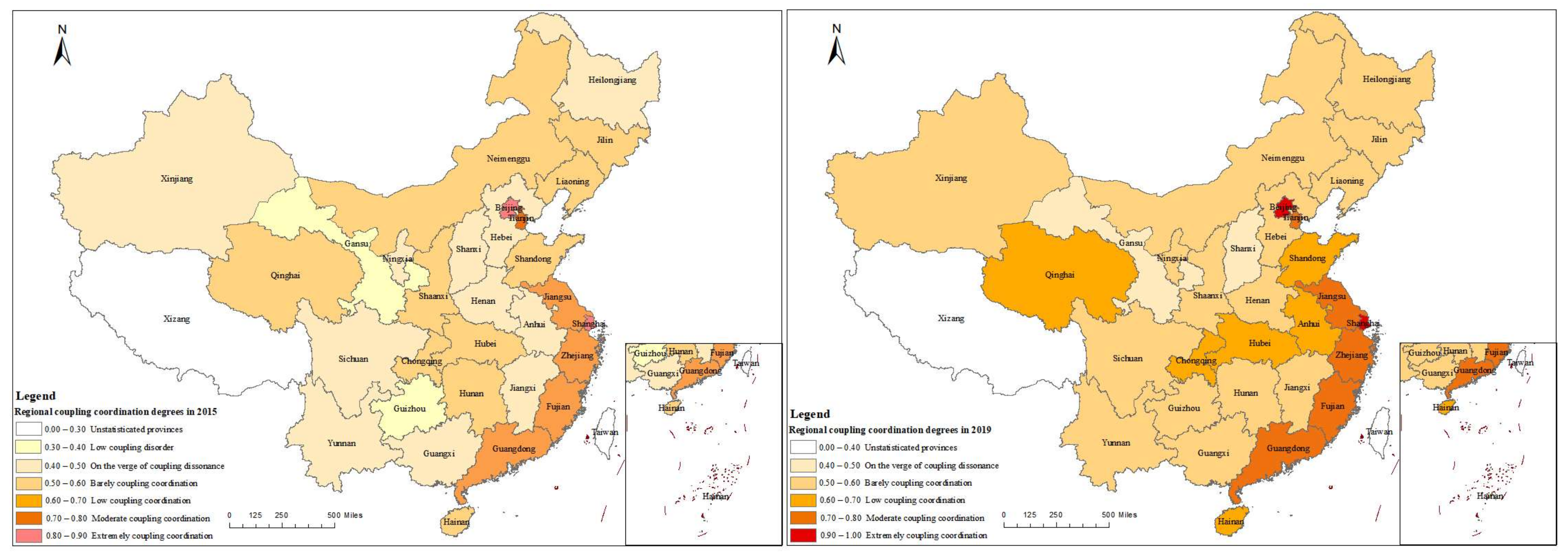
• The coupling coordination degree in each provincial-level administrative region increased in the period 2015–2019. The top five provinces in terms of the coupling coordination degree are Beijing Municipality, Shanghai Municipality, Tianjin Municipality, Jiangsu Province, and Zhejiang Province. In 2019, Guizhou, Guangxi, Ningxia, Gansu, and Shanxi ranked the bottom five provinces in terms of low-carbon economic development. Therefore, it is essential to strengthening policy formulation to promote economic development, industrial structure optimisation, energy structure adjustment, and low-carbon consumption reduction.
• The coupling coordination levels of the 30 provinces in 2015 included low coupling disorder, on the verge of coupling dissonance, barely coupled coordination, low coupling coordination, moderate coupling coordination, and highly coupling coordination. In 2019, two provinces upgraded to extremely coupling coordination. During the study period, the overall coupling coordination level increased, indicating that the coupling coordination degree between regional economic development and energy consumption low-carbonisation in China gradually increased over time. However, in 2019, the proportion of provinces with coupling coordination below the moderate coupling coordination level remains high at 76.56%. Therefore, in future policymaking, policymakers should take the imbalance and inadequacy of development between regions into account, giving more priority to enhancing the coordinated development of economic and low-carbon energy consumption in these provinces with a lower level of coupling.
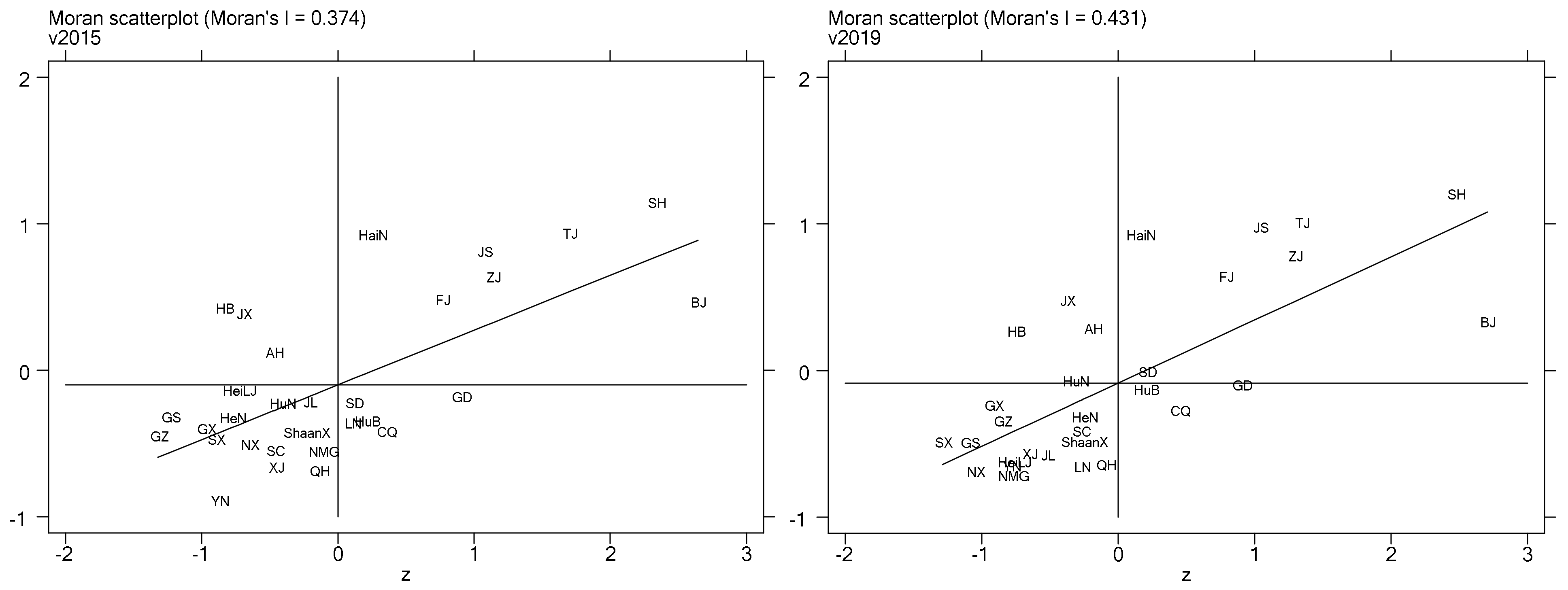
• The global SAR results indicate that the global Moran’s I indices of the coupled coordination from 2015 to 2019 are significantly correlated within the 95% confidence interval, and the I values are greater than zero, indicating that the coupled coordination is positively correlated in terms of the spatial distribution and has significant spatial clustering characteristics. The global Moran’s I index value increased from 0.252 to 0.315 during the study period, indicating that the spatially positive correlation between the regional economic development and low-carbonisation of energy consumption became more significant. Therefore, in future policy formulation, the role of the spatial correlation effect of coupling coordination should be given full play to strengthen the complementary links and positive influence between provinces and neighbouring provinces in terms of economy, society, energy, industry, technology, and talent.
• The local SAR results show that the local Moran’s I indices of the 30 provincial-level administrative regions in China are distributed in the first and third quadrants during the study period, indicating that the coupling coordination of most provincial-level administrative regions exhibits a strong positive spatial correlation with the neighbouring provinces. The eastern and western provincial-level administrative regions are mainly distributed in the H–H and L–L agglomeration areas of the Moran’s scatterplot, respectively. In the study period, the spatial correlation pattern of the regional coupling coordination has a high stability, with most regions not leaping, and two of the 30 provincial-level administrative regions leaping to the first and third quadrants from 2015 to 2019. This finding indicates that the positive spatial correlation effect of the coupling and coordination of the system is strengthened. There are significant differences in the spatial distribution of the coupling coordination degree among provinces, as shown by the clustering characteristics of provinces with higher and lower levels of coupling, while the driving effects of some provinces with higher coupling levels on neighbouring provinces are limited. In this sense, there is no doubt that issues such as the uneven development of regional economies, societies, energy consumption, and the environment have hindered the smooth development of China’s low-carbon economy. Therefore, provincial districts should promote the process of low-carbon economic development based on the status quo and difficulties of local development, and strengthen inter-provincial policy interchange and mutual promotion, dynamic flow of production factors, emission as well as carbon reduction in energy consumption, industrial integration and development, and synergistic innovation in science and technology, in order to narrow regional differences comprehensively, and to advance the balanced development of China’s green, low carbon, and circular economic system.
• The results of the decomposition of the effects of the SDM show that the improvement in the regional economic level, advancement of urbanisation process, low coal consumption structure of energy, and increased level of investment in science and technological innovations promote the increase in the coupling degree. As the core of policy formulation and implementation, the factors elaborated above are critical to promoting the development of a high-quality low-carbon economy. The low coal consumption structure of regional energy and the investment level in science and innovation impose a significant positive spatial spillover effect on the coupling degree of neighbouring provinces. Therefore, it is crucial to step up in-depth cooperation between local governments in the fields of energy supply and demand, clean energy technologies, and scientific research and innovation, to give full play to synergy-driven effect. The advanced industrial structure adversely influences the coupling degree. This phenomenon occurs owing to the heterogeneity of regional industrial development in terms of coordination, balance, and maturity, and interactive relationship between industrial structure transformation, economic growth, and energy consumption in different regions. Given the differences in regional resource endowments and disparate stages of economic development, on the one hand, it is essential for provinces to implement the strategies of industrial structure transformation and upgrading in accordance with local conditions, and the enhancement of local government governance capacity and policy support are accelerated, to give full play to the positive role of local governments in energy conservation and emission reduction during industrial structure transformation [50]. On the one hand, in provinces dominated by heavy industries, it is necessary to accelerate the promotion of energy conservation and carbon reduction in traditional industries, contribute to technological innovation and equipment upgrading of advanced production capacity, and eliminate outdated production capacity with high energy consumption as well as pollution. Regarding the provinces with new technology-based industries as the primary driver of development, it is necessary to further integrate high-quality elements, reinforce the investment in scientific research, and step up the transformation efficiency of R&D and capabilities and achievements to encourage the green, low-carbon and high-quality development of technology-intensive industries.

Several limitations of this study can be addressed and deepened in future work. There are several limitations in this study which should be addressed in future research. Firstly, in this paper, the spatiotemporal coupling effect of regional economic development and de-carbonisation of energy is investigated from the provincial perspective, which could be extended to the urban discrepancy to analyse the spatiotemporal characteristics in more detail. Second, the evaluation index system needs to be further improved. For example, the dimensions of the regional ecological environment can be taken into further account, and indicators for measuring the development of clean energy can be added to the impact of energy structure. Third, several key factors related to the coupling coordination between the economic development level and low-carbonisation of energy consumption have been selected in this paper to identify its driving effect, but the government policy, environmental regulation, and other factors should be further considered in future research.

References

- Dou, R.Y.; Liu, X.M. Study on the relationship between energy consumption and economic growth in typical resource-based regions of China. China Popul. Resour. Environ. 2016, 26, 164–170. [Google Scholar]
- He, Z.; Yang, Y.; Song, Z.Y.; Liu, Y. The mutual evolution and driving factors of China’s energy consumption and economic growth. Geogr. Res. 2018, 37, 1528–1540. Available online: https://kns.cnki.net/kcms/detail/detail.aspx?dbcode=CJFD&dbname=CJFDLAST2018&filename=DLYJ201808006&uniplatform=NZKPT&v=jxZEPYyDYor_hoGHUq6HoF7XXjyjqJqm6e-uAfBIjfkwBb7tcvVy3Cqv44sne7nn (accessed on 3 December 2021).
- Bekun, F.V.; Emir, F.; Sarkodie, S.A. Another look at the relationship between energy consumption, carbon dioxide emissions, and economic growth in South Africa. Sci. Total Environ. 2019, 655, 759–765. [Google Scholar] [CrossRef] [PubMed]
- Shahbaz, M.; Hoang, T.H.V.; Mahalik, M.K.; Roubaud, D. Energy consumption, financial development and economic growth in india: New evidence from a nonlinear and asymmetric analysis. Energy Econ. 2017, 63, 199–212. [Google Scholar] [CrossRef]
- Mirza, F.M.; Kanwal, A. Energy consumption, carbon emissions and economic growth in pakistan: Dynamic causality analysis. Renew. Sustain. Energy Rev. 2017, 72, 1233–1240. [Google Scholar] [CrossRef]
- Li, G.Z.; Huang, Q.J. Study on the coordinated development of energy—Economy—Environment -technology system in Beijing-Tianjin-Hebei. Stat. Decis. 2021, 37, 129–131. [Google Scholar] [CrossRef]
- Lu, J.; Chang, H.; Wang, Y. Dynamic evolution of provincial energy economy and environment coupling in China’s regions. China Popul. Resour. Environ. 2017, 27, 60–68. [Google Scholar]
- Miao, Y.; Xing, W.J.; Bao, J.Q. Low-Carbon Index Evaluation System of the Urban Energy Structure and Its Attainment. Ecol. Econ. 2016, 32, 53–57. [Google Scholar]
- Fu, J.X.; Liu, Y.Q. A Study on China’s Low-Carbon Energy Development:A Case Study of Beijing. Macroeconomic 2020, 164–175. [Google Scholar] [CrossRef]
- Sun, Q.; Wu, Q.S.; Li, S.Y.; Li, X.J. Measurement on China’s Urban Low-carbon Development Performance Index. Stat. Decis. 2021, 37, 75–79. [Google Scholar] [CrossRef]
- Meng, F.S.; Zou, Y. The Optimization Degree Evaluation of Energy Structure Base on the SPA-TOPSIS. Oper. Res. Manag. Sci. 2018, 27, 122–130. [Google Scholar]
- Jiang, W.J. Analysis of coupled population-regional economic-environmental development coordination. Stat. Decis. 2017, 15, 101–104. [Google Scholar] [CrossRef]
- Pang, S.L.; Wu, M.Y. Research on the coupled and coordinated development of higher education scale and regional economy in China. Stat. Decis. 2021, 37, 109–112. [Google Scholar] [CrossRef]
- Guo, H.X. The Coal Resources in Shanxi Province and Study on The Relationship between The Coupling of The Regional Economic Development. Master’s Thesis, Shanxi Agricultural University, Jinzhong, China, 2015. Available online: https://kns.cnki.net/KCMS/detail/detail.aspx?Dbname=CMFD201502&filename=1015635110.nh (accessed on 17 December 2021).
- Statistics Bureau of the People’s Republic of China. China Statistical Yearbook, 2016–2020. Available online: http://www.stats.gov.cn/ (accessed on 2 May 2022).
- Statistics Bureau of the People’s Republic of China. Statistical Yearbook of China’s Fixed Assets Investment (China’s Investment Field), 2016–2020. Available online: http://www.stats.gov.cn/ (accessed on 2 May 2022).
- Statistics Bureau of the People’s Republic of China. China Energy Statistical Yearbook, 2016–2020. Available online: http://www.stats.gov.cn/ (accessed on 2 May 2022).
- Statistics Bureau of the People’s Republic of China. China Census Yearbook, 2016–2020. Available online: http://www.stats.gov.cn/ (accessed on 2 May 2022).
- Carbon Emission Account & Datasets. Emission Inventories for 30 Provinces, 2015–2019. Available online: https://www.ceads.net.cn/ (accessed on 2 May 2022).
- Zhao, R.F.; Wang, X.N. Comparison of Regional Innovative Abilities in Bejing-Tianjin-Hebei Area Based on Overall Entropy Method. China Bus. Mark. 2017, 31, 114–121. [Google Scholar] [CrossRef]
- Luo, Y.S.; Lu, Z.N.; Zhao, X.C. Evaluation and spatial statistical analysis of the level of intellectual property resources in Chinese provinces. Stat. Decis. 2020, 36, 62–66. [Google Scholar] [CrossRef]
- Li, Y.J.; Zhang, L. Dynamic Evaluation of Industrial Ecologization Level in the Upper Reaches of the Yangtze River Base on Overall Entropy Method. Ecol. Econ. 2021, 37, 44–48.56. [Google Scholar]
- Zong, X.; Yang, H. Analysis on the Spatio temporal Coupling Relationship and Driving Forces of New Urbanization and Urban Low Carbon Development. Ecol. Econ. 2021, 37, 80–87. [Google Scholar]
- Miao, L.; Wen, B.X.; Wen, Q.Y. Coupling and Coordination Relationship Between Local Financial Investment in Education and Economic Development Level in China. Econ. Geogr. 2021, 12, 1–9. [Google Scholar] [CrossRef]
- Li, M.; Mao, C. Spatial-Temporal Variance of Coupling Relationship between Population Modernization and Eco- Environment in Beijing-Tianjin-Hebei. Sustainability 2019, 11, 991. [Google Scholar] [CrossRef]
- Zhang, Y.; Su, Z.; Li, G.; Zhuo, Y.; Xu, Z. Spatial-Temporal Evolution of Sustainable Urbanization Development: A Perspective of the Coupling Coordination Development Based on Population, Industry, and Built-Up Land Spatial Agglomeration. Sustainability 2018, 10, 1766. [Google Scholar] [CrossRef]
- Yu, X.X. Spatio-temporal analysis of the coupled economic-social-technological-resource coordinated development. Stat. Decis. 2017, 9, 127–131. [Google Scholar] [CrossRef]
- Gao, H.G.; Luo, Y. Coupled measurement of urbanization and ecological environment quality in the Yangtze River Economic Zone. Stat. Decis. 2021, 37, 111–115. [Google Scholar] [CrossRef]
- Chen, Q. Advanced Econometrics and Stata Applications; Higher Education Press: Beijing, China, 2014; Volume 4, pp. 578–579. [Google Scholar]
- Liang, S.; Gao, X.L.; Wang, S.Y. Evaluation and Spatial Measurement Study of Energy Security, Energy Consumption and Pollutant Emissions; China Water Conservancy and Hydropower Press: Beijing, China, 2021; Volume 1, pp. 107–114. [Google Scholar]
- Anselin, L. Spatial Econometrics: Methods and Models; Kluwer Academic Press: Dordrecht, The Netherlands, 1988; pp. 223–239. [Google Scholar]
- Guo, Y.; Fan, B.N.; Long, J. Practical Evaluation of China’s Regional High-quality Development and Its Spatiotemporal Evolution Characteristics. Quant. Tech. Econ. 2020, 37, 118–132. [Google Scholar] [CrossRef]
- Rey, S.J. Spatial Empirics for Economic Growth and Convergence. Geogr. Anal. 2010, 33, 195–214. [Google Scholar] [CrossRef]
- Sun, Y.; Zheng, S.L.; Gan, K.Q. Research on Measurement and Spatial Pattern of National Quality Infrastructure Development in China. Sci. Technol. Manag. Res. 2021, 41, 191–198. [Google Scholar]
- Zhang, S.S. A few thoughts on undertaking industrial transfer in Hebei Province. West. Leather 2018, 40, 117. [Google Scholar]
- Fan, H.J.; He, S.J. Construction and Measurement of Evaluation System of Modern Industrial System. Reform 2021, 8, 90–102. [Google Scholar]
- Liu, B.; Wang, A. Study on the Evaluation and Construction Path of Modern Industrial System: Taking Shandong Province as an Example. Inq. Econ. Issues 2020, 5, 66–72. [Google Scholar]
- Elhorst, J.P. Matlab Software for Spatial Panels. Int. Reg. Sci. Rev. 2014, 37, 389–405. [Google Scholar] [CrossRef]
- Zhong, R.Y.; Zeng, J.H. The Impact of Digital Economy on Household Consumption—Empirical Analysis Based on the Spatial Durbin Model. Inq. Econ. Issues 2022, 3, 31–43. [Google Scholar]
- Lu, T.T.; Zhu, Z.Y. The Influence of Artificial Intelligence on Labor Income Share from the Perspective of Space—Analysis Based on Static and Dynamic Space Durbin Model. Inq. Econ. Issues 2022, 5, 65–78. [Google Scholar]
- Mao, Z.G.; Wu, U.M.; Xie, C. Spatial Pattern and Influencing Mechanism of Consumption Level in Yangtze River Delta Urban Agglomeration. Econ. Geogr. 2020, 40, 56–62. [Google Scholar] [CrossRef]
- LeSage, J.; Pace, R.K. Introduction to Spatial Econometrics; CRC Press: Boca Raton, FL, USA, 2009. [Google Scholar]
- Xu, D.Y.; Liu, X.H. Impact of Infrastructure on the Real Exchange Rate: Evidence from China’s Provincial Data by Spatial Dubin Model. World Econ. Stud. 2022, 3, 33–53+134. [Google Scholar] [CrossRef]
- Brunt, L.; García-Pealosa, C.; Boucekkine, R. Urbanization and the onset of modern economic growth. Econ. J. 2021, 132, 512–545. [Google Scholar] [CrossRef]
- Poumanyvong, P.; Kaneko, S. Does urbanization lead to less energy use and lower CO2 emissions? A cross-country analysis. Ecol. Econ. 2010, 70, 434–444. [Google Scholar] [CrossRef]
- Sharma, S.S. Determinants of carbon dioxide emissions: Empirical evidence from 69 countries. Appl. Energy 2011, 88, 376–382. [Google Scholar] [CrossRef]
- Zhang, A.H.; Huang, J. An Empirical Study on the Effects of Urbanization on the Efficiency of Development of Regional Low-Carbon Economy. J. Shaanxi Norm. Univ. (Philos. Soc. Sci. Ed.) 2015, 44, 76–82. [Google Scholar]
- Xiao, Y.F.; Wu, Y.; Zhou, W.Q. Can new urbanization construction promte low-carbon technology innovation. J. Chongqing Univ. Technol. (Soc. Sci.) 2019, 33, 22–32. [Google Scholar]
- Cui, J.N.; Shi, L.Y.; Xie, B.J. Can the Convergence of Technology and Industry Drive the Development of Regional Economy—A Dynamic Spatial Durbin Model Based Studyl. J. Harbin Univ. Commer. (Soc. Sci. Ed.) 2022, 02, 15–25. [Google Scholar]
- Fu, Z.H.; Jing, P.Q. Local government governance capacity, industrial structure transformation and energy consumption. Stat. Decis. 2022, 10, 162–166. [Google Scholar] [CrossRef]
- Zhang, Z.Q.; Liu, J.P. Analysis on the inverted “U” relationship between advanced industrial structure and energy intensity. Coal Eng. 2021, 53, 189–192. [Google Scholar]
- Liu, Y.; Xiao, H.; Zikhali, P.; Lv, Y. Carbon Emissions in China: A Spatial Econometric Analysis at the Regional Level. Sustainability 2014, 6, 6005–6023. [Google Scholar] [CrossRef]
- Liu, Y.; Xiao, H.; Zhang, N. Industrial Carbon Emissions of China’s Regions: A Spatial Econometric Analysis. Sustainability 2016, 8, 210. [Google Scholar] [CrossRef]