Multiple Industrial Induction Motors Fault Diagnosis Model within Powerline System Based on Wireless Sensor Network

Abstract

The voltage supply of induction motors of various sizes is typically provided by a shared power bus in an industrial production powerline network. A single motor’s dynamic behavior produces a signal that travels along the powerline. Powerline networks are efficient at transmitting and receiving signals. This could be an indication that there is a problem with the motor down immediately from its location. It is possible for the consolidated network signal to become confusing. A mathematical model is used to measure and determine the possible known routing of various signals in an electricity network based on attenuation and estimate the relationship between sensor signals and known fault patterns. A laboratory WSN based induction motors testbed setup was developed using Xbee devices and microcontroller along with the variety of different-sized motors to verify the progression of faulty signals and identify the type of fault. These motors were connected in parallel to the main powerline through this architecture, which provided an excellent concept for an industrial multi-motor network modeling lab setup. A method for the extraction of Xbee node-level features has been developed, and it can be applied to a variety of datasets. The accuracy of the real-time data capture is demonstrated to be very close data analyses between simulation and testbed measurements. Experimental results show a comparison between manual data gathering and capturing Xbee sensor nodes to validate the methodology’s applicability and accuracy in locating the faulty motor within the power network.

1. Introduction

Induction machine fault identification has gained attention in the past two decades. Because of this, there has been a general increase in the consistency of the production plant [1]. The process of an advanced manufacturing electricity network is typically impacted in some way by a selection of induction motors whose sizes range from extremely small to extremely large. The operation of the whole system may be adversely affected as a result of the combined effects of these groups of motors. The combined impact of each of these distinct electrical machines can have a substantial effect on the network’s ability to maintain its stability [2].

Induction motor faults often involve rotating parts and electric drives. The behavior of induction motors can be perceived using a variety of methods, some of which have been accepted for publication in academic journals [3], while others are available for purchase from various vendors. Nevertheless, there are still engineers in the industry who are griping about consistent, regular, and unforeseen motor faults. Nevertheless, there are some faults that are difficult to identify in their early stages, and the symptoms of these faults only become apparent as they accelerate the component of induction motors ageing [4,5].

Various mechanical operation properties can be used to monitor a motor’s health, including leakage, thermal monitoring of trouble spots, chemical content, acoustics, machine power management, machine axial leakage flux, torque, machine acoustic emission signals, and induction machine signatures [6,7]. The method of rotor circuit electric current interpretation is particularly well known among these techniques. Because of the factors listed below, the Motor Current Signature Analysis (MCSA) is a method that has garnered a lot of attention [8]:

• The electric current signal can be simplified.
• There is no requirement for motor access in order to carry out remote monitoring.
• A variety of other monitoring applications make use of current and voltage sensors that are not overly expensive.

MCSA is less accurate than vibration monitoring. External interference is caused by additive noise, motor operation, and plant noise [3]. These noises can mimic abnormal signal behavior. Signature analysis is complicated. The manufacturing industry seems to need reliable electronic fault diagnosis alternatives to prevent unnecessary decision-making confusion [9].

The power output and the electrical currents are the parameters that are most frequently used for the sign of fault symptoms inside the system of industrial motors. The existence of electric current is what distinguishes the procedure of the voltage in induction motors from other types of motors. The voltage at the electric connector is a function of its supply voltage and the electricity network’s configuration. As a consequence of this, voltage, when viewed in isolation, can in fact be considered an indicator of the reliability of an induction machine. In addition to this, the structure of the motor power grid and the current that it garners are both factors that have an impact on the voltage that is supplied [10]. On either hand, taking the readings of both the current and the voltage together is likely to be the most effective diagnostic method.

MCSA is a simpler, more effective method for diagnosing induction motor faults [4,5,6]. This technique estimates the existence of pre-recorded fault signatures using a pattern recognition processing information to the strong electric signal of motor drives in order to make the determination [11]. In recent years, studies have reported industrial motor problems and claimed MCSA is an effective diagnostic technique. Interference between the various parts of the motor network is the most significant obstacle that must be overcome with MCSA. It has been suggested to use a few different methodologies in order to boost reliability and cut down on the possibility of uncertainty when making decisions. On the other hand, interference from neighboring motors might produce a frequency spectrum that is analogous to the pattern of allegedly faulty components. In addition, the majority of electric motor’s low-power components are unaffordable using these methods due to their high cost. According to the findings of a review and survey, using a solitary monitoring system for a significant number of low and medium power electric motors is not financially viable [12]. Figure 1 shows an MCSA-based top-down fault-diagnosis framework. This framework has many processes.

As can be seen in Figure 1, the processes of data acquisition, the application of filters, signal conversion, the application of morph methods, and fault diagnosis each involve different steps. There are several individual aspects that can be used for data acquisition. However, the signal should be transformed and sampled most of the time by means of an electric current sensor or a voltage transformer. Therefore, the frequency of 50 hertz is taken into consideration to include the typical functioning of induction motors. Next, remove high-frequency constituents of the electronic signals so that they are irrelevant to fault diagnosis [13]. A low pass filter converts the analogue signal’s frequency spectrum to digital. Data processing classifies a sufficient quantity point. In summary, an approach for defect detection is needed to find the challenge, and a post-processing methodology is needed to assess the condition of the motor that triggered the warning alarm.

As can be seen in Figure 2, a typical process for monitoring systems and fault diagnosis/prognosis is broken down into four stages: data gathering, extraction of features, diagnosis/prognosis, and decision making.

The remaining parts of the paper can be divided into the following sections: In Section 2, a state-of-the-art literature review is presented to support the concept. Section 3 illustrates the proposed Distributed Motor Network Model along with the mathematical modelling. Multi-motor testbed environment using WSN is presented in Section 4. Next, Section 5 describes the experimental multi-motor testbed, the case study-based experiment results, and the paper’s conclusion and future direction are included in Section 6.

2. Related Works

Scientists in industry and academia have turned their focus in recent decades to stator current testing, or MCSA as it is commonly known. When compared to other forms of motor condition-based maintenance (such as vibration), it can provide a similar indication without having to open the motor itself [7]. Motor protection usually involves measuring stator current. Measurement of current becomes a built-in feature of the drive systems, making it available for no additional charge. To detect faults with current signature analysis, there are three basic methods to choose from. Frequency spectral analysis, negative-positive and steady state aspects, and Park’s vector three-phase high voltage depiction [8].

Over the course of the past few decades, a great number of techniques for diagnosing problems with induction motors have been developed, and many of these techniques have been described [14]. MCSA is the method that is utilized most frequently for the purpose of fault diagnosis [10]. FFT signature analysis is used to detect the induction motor faults shown in Figure 3. In general, induction machines have a symmetrical design. Faults in the equipment will have a big effect on its consistency and can lead to things like torque pulsation that keeps getting worse, uneven impedance voltages and current flowing, more shortfalls and less performance, less shaft torque, and more space harmonics [3]. In the context of an industrial setting, failure modes for induction motors can be broken down into four primary categories [12]. The potential issues that may be present and the symptoms that are associated with them are presented in Figure 3.

Altaf et al. [15] present a comprehensive comparison survey that goes into great detail. This exhaustive survey is a compilation of data from a variety of sources, some of which include approximately 80 journal papers that have been presented in IEEE and other reputable electrical engineering journals. The results of the survey are summarized in Figure 4, which can be found here.

Bearing-related faults account for the vast majority of failure modes (52.5%). When the fault with the bearings and the faults with the stator are considered together, they account for more than 87.5% of the overall faults that are already present [16]. However, faults that are related to bearings are typically caused by mechanical and vibrational issues [17]. Therefore, the scope of this study is limited to the rotor, air gap eccentricity, and associated faults. This is because rotor-related failures are the easiest in induction motors, which is why this is the case. This can be accomplished through the utilization of MCSA with the double slip intensity harmonic components of the fundamental frequency [18].

In order to achieve complete energy balance, Liu et al [19] suggests connecting the nodes using the electricity supply line. The briefest length of powerline is also postulated as associated with fixed. Based on energy stability, the perfect sequence number for transmitted data is envisioned, which minimizes energy usage. An energy-efficient wireless sensor network is possible with the suggested protocol, according to the analytical model. A novel IMD-EACBR process, which was introduced by other research [20] and intended to maximize energy effectiveness and longevity of wireless sensor nodes, has been developed.

Bengherbia [21] presented replacing a commercial sensor network node FFT technique with a fixed ADALINE cnn architecture applied on an embedded system. Estimating harmonic currents in a rotating machine reduced completion time and net flow. The XSG developed the IP-simple core’s block layout. It is a MicroBlaze multicore processor in the wireless mesh network.

3. Distributed Motor Network Model

Figure 5 depicts a typical configuration for an industrial multi-motor powerline network, and this study explains the core idea of malfunction signal integrity and recognition via the primary powerline. This study also takes into account the primary powerline. This provides an environment that is capable of conducting signals so they can relocate through the subnet and influence other machine behavioral sensory information [17]. This, in turn, is useful because it creates an environment that is good at conducting signals. Several elements of a configuration of integrated induction motors using an integrated supply bus have been mulled over and taken into consideration at this point. It is necessary to take into account a number of different measuring points in order to perceive the behavior of induction motors. Multi-motor frameworks are being considered to advance this concept. This model, as shown in Figure 5, consists of a primary powerline, sub-segment resistive load, and connected motors. A separate type of measurement locations was supposed during certain positions to monitor the behavior of each electrical machine in the same bus throughout the order to assess the diagnostic accuracy and examine the observational data. This was done in order to make a determination regarding the prognosis.

Independent and consolidated analyses of every fault pattern have been addressed [12], and they were performed while using a high and low induction machine network. It is a direct result of the transmission of fault signals all throughout the powerline network. In addition to this, it highlights the significant influence that faulty signals can have, not only on neighboring motor drives within the same bus, but also on motors in other buses. This process of signal propagation could result in changes to the pattern behavior of each neighboring motor, which would subsequently lead to confusion regarding the location of the original source of failure indices. When faulty data are received in a neighboring motor, the motor network must cancel the noise and filter the faulty signal from the targeted motor. The faulty signal is only detected then. This makes signal diagnosis easy. To expand the pattern matching scheme’s application and ensure it uses all networked sensing points, networked MCSA was chosen.

Due to the obvious nonlinear response of an electric motor in an interconnected powerline network, a time-variant methodical solution is recommended to eliminate suspicious results. To analyze each bus’s multiple-motor frequency band, follow these steps [13].

• First, collect information from the sensors that are connected to the powerline network. Significant sideband spectral points as well as magnitude measurements are taken into consideration as possible future motor fault signals.
• Next, collect sideband frequencies at various sensing points throughout the bus. Sensors and data have their own thresholds. After taking out from the frequency spectrum any effective interpersonal sideband components that do not fit with the key patterns of the frequency band, the remaining signal would then be categorized relative to a reference fault pattern.
• Thereafter, it is useful to collect all of the necessary sideband magnitude and phase values at a number of different sensing points. If the measured amplitudes are significantly outside of the normal range, the problem is most likely located in the motor itself or in a neighboring motor that is connected to the same bus. Otherwise, other buses may be sending the signal [14].
• The physical distance separating the various buses and motors affects both the intensity of the faulty harmonic components at every motor as well as their level of influence. If a high-power motor on the same bus perpetuated the defective signal, after which similarly powered motors on the bus would get the same influence, with only a minor difference in amplitude value, just a low-power motor may have a greater influence than the other motors. This demonstrates that they are lacking in some way or another. This spectrum has been detected emanating from a number of different motors. If a low-power machine propagates a faulty signal, a high-power machine on the same bus will have less influence (HP). This results in a degree of uncertainty regarding whether the alleged sideband components are being generated by their motor or beginning to develop themselves from other sources. Because of this kind of confusion, it might be impossible to pinpoint the true origin of the fault indices.
• After analyzing multiple sensing points, the next step in locating the malfunctioning motor in a network is to choose the area of the bus that is under suspicion. Examine all bus motor signatures to find the ambiguous motor [12]. Due to a defective sideband, the actual motor speed must be evaluated and compared to the synchronized insights on their physical behavior. If the speed is normal, this sideband frequency probably refers to other motors. You cannot tell by speed alone if a motor is faulty. Significant frequency points will be used to start generating a fault factor based on suspected faults.

Figure 6 depicts the multi-path spread of the signal as well as the sensing points. This figure contains various sensing points of the signal propagation $\left(S_1,S_2,\dots , S_n\right)$ dispersed across a motor network and refers to the respective sub-buses. Each link is comprised of four different branches, has a diverse route path $\left(R_1,R_2,\dots , R_n\right)$ amid multiple buses path $\left(L_1,L_2,\dots , L_n\right)$, and demonstrates the impedances of every bus span at every sensing point along with others. If the distance among both industrial motors is known, different combinations of sensing coordinates can be predicted to analyze fault strength at each point. It helps identify signal origin direction. In the case of unknown motor-to-bus distance, sensing only each point’s value is insufficient to distinguish fault signals. An attenuation component would relieve this concern and pinpoint faulty motors in the network. This fault index shows the relative strength of any fault signal.

Table 1. Conceivable sensor locations within a distributed powerline network.

Interconnection of the Various Buses	Path Segment	Range between Buses	Multiple Sensor Combinations
$B_1\to B_2$	$R_1\to R_2\to \dots \to R_3$	$L_1+L_2+L_3$	$S_1\to S_2\to S_3\to S_4$ $S_2\to S_1$ $S_2\to S_3\to S_4$ $S_3\to S_4$ $S_3\to S_2\to S_1$ $S_4\to S_3\to S_2$ $S_4\to S_3\to S_2\to S_1$
…	…	…	…
$B_1\to B_2\to B_3\dots \to B_n$	$R_1\to R_2\to \dots \to R_{n-1}$	$L_1+L_2+\dots +L_{n-1}$	$S_1\to S_2\to \dots \to S_{n-1}$

shows a fault index as numerous sensing points between motor locations.

3.1. Mathematical Model for Faulty Signal’s Effect on Electric Current Spectrum

Figure 6 is provided as a point of reference for the purpose of formulating a theoretical formulation for the propagation and impact on faulty signals. In this diagram, one of the motors, denoted by the symbol $\left(M_{1.3}\right)$ is supposed to be defective. This motor is sending out a rotor bar failure signal and may be responsible for a decrease in the overall current level.

The equation that describes the voltage-drop phasor $V_{\mathrm{drop}}$ for a subdivision of a powerline that consists of electric current and impedance is as follows [12]:

$$V_{\mathrm{drop}}=I·Z$$

(1)

In embedded environments, the functional voltage is the mathematics transformation between sending and receiving [4].

$$Vo{l}_{\mathrm{main}\text{-}\mathrm{line}}=\left(Vo{l}_{B1},Vo{l}_{B2},Vo{l}_{B3},\dots \dots \dots .,Vo{l}_{Bn}\right)$$

(2)

$$Vo{l}_{\mathrm{main}\text{-}\mathrm{line}}={\displaystyle \sum }_{m=1}^{n}Vo{l}_{\mathrm{main}\text{-}\mathrm{line}\to \mathrm{m}}$$

(3)

where, $Vo{l}_{\mathrm{main}\text{-}\mathrm{line}}$ is the voltage that is produced by the power system network as a whole and $\mathrm{m}$ is the manifestation of current for the $m$th induction machine within, respectively, of the all sub-buses. The following is the voltage that is produced as a result of the motor (M_1.3) being connected to sub-bus 1:

$$V_{B_1\to M_{1.3}}=I_{M_{1.3}}·Z_{M_{1.3}}$$

(4)

The electric current signal generated by motor 3 has an effect on the surrounding motors ($M_{1.1}$ and $M_{1.2}$) in the same bus area as $M_{1.3}$. That the electrical current is passed in different motors is observed using mirror theory [15].

Calculating the effect that this will have on the primary electricity bus as well as the secondary buses should not be too difficult. Because of the influence of this faulty signal on other motor drives, there may be signal corruption. This exposes some of the problems. It has the potential to alter the characteristics of a variety of features, which could lead to output impedance drops in almost the same path in the powerline network [16]. Through all the electrical charge reflection hypothesis, a defective signal can conveniently be propagated to neighboring motors at the given power frequency. The mathematical model [17] estimates motor static impedance at the given power frequency:

$$Z_{B_n{M}_n}=\sqrt{\frac{V_{sf}}{P_{sf}}}.$$

(5)

where, $V_{sf}$ & $P_{sf}$ are constants that are defined for the purpose of frequency filtering.

If there is a problem with the rotor, it will cause an imbalance in the electric current flowing through the rotor and will result in an opposite magnetic field frequency. This frequency is related to a factor at frequency $-s{f}_1$ that has to do with an opposite electric current sequence [18]. This electric current sequence in reverse will be evidenced on the stator winding as well, which will result in left-side frequency bands $\left(1-2s\right)f_1$, as shown in Figure 7 below.

3.2. System for Fault Diagnosis at the Motor Level

Isolated fault decision-making can affect fault type identification and localization in a distributed system’s network. Fault signal propagation, noise, and available travel paths on a powerline network can cause diagnostic confusion for live listening at adjacent nodes as well as multiple faults at a number of different nodes. Next, the powerline network needs a fault location detection and recognition. Fault detection at each motor level is depicted in Figure 8 through the development of a systematic diagnostic framework.

Figure 8 depicts a WSN-based distributed fault diagnosis framework for multiple-motor architecture. It shows activities for motor level diagnosis. Spectrum data acquisition requires many components. All motors collect the signal via a current or voltage transducer or transformer. The resonance frequency (50 Hz) is used to observe motor operation. Next, high-frequency signal components not needed for diagnosis are removed. A threshold value is used to remove signal noise. The threshold level depends on site noise, motor network structure, and accuracy. Analog-to-digital converters transform sampled data into digital signals. Estimating the waveform’s frequency spectrum follows digitization. Using a computational technique, spectrum signature patterns are made from the waveform signal’s significant components. Frequency spectrums form most signatures and fault patterns.

4. Multi-Motor Test-Bed Environment Using WSN

The distributed signature analysis is depicted in Figure 9 and includes a number of sensing points in order to monitor the electric current signal. An evaluation of distributed signatures might be the best choice if you want to obtain the most trustworthy data possible for fault diagnosis. It may also clarify network noise fault symptoms. In addition, we will discuss how to identify defective powerline motors. Signal processing aids in estimating the effect of fault signals on the network motor current.

Electric current impulse fading relates to structured methodologies that predict fault signal diffusion and recognizes signal path routes. The framework shows WSN node’s role in transmitted signature analysis. Wireless nodes would collect data, generate potential fault signatures, identify noise levels in signals, diagnose fault error symptoms, observe the behavioral patterns of nearest neighbors in real time, and notify the coordinator node of suspicious situations. This distributed diagnosis strategy will provide early signs of fault conditions for in-network electric motor without a direct evaluating method.

Multiple motors were used in an experimental network to show how faulty inputs propagate through an electrical network and how fault types are perceived in the lab. This was done in order to demonstrate the recognition of fault types. Within the confines of the same primary powerline, two different sized single-phase induction motors were connected. For the purpose of modelling the multi-motor network, a total of nine induction motors were utilized. Figure 10 demonstrates that all these machines were distributed across three separate sub-buses. Each bus had two-size induction motors. Two 15-W (Model No. S7I15GE-S12) and one 25-W motors (Model S8I25GE-S12) were used. Various sizes of induction motors were used to compare high and low power motors. Each motor had a data-collecting point. Torque from the brakes caused motor vibration. Each assessment takes a moment to store in a flash drive at 25,000 samples per second. Applying brake vibration and rotor misalignment artificially created faults.

During this particular test, a range of different practical experiments were carried out. The Tektronix oscilloscope (TDS2012B) must have been utilized so that the data from the measurements could be saved onto a flash drive. At the same time that manual data was being captured, current probes made by Tektronix (A622) were used to record the information about the electric current. A digital infrared tachometer with the model number ST-6234B was utilized in order to determine the frequency of each motor. All of the data from the measurements were saved in a distinct Excel spreadsheet file corresponding to each motor.

Figure 11 describe the experimental configuration and microcontroller specifications with a current sensor for Xbee Arduino analysis.

The software for this system is split into two parts. It is necessary to program Arduino boards so that they can measure and transmit sensor readings. Arduino boards are configured in C to log sensor data and analyze it per user request. Load current sensors use different reading methods. Arduino built-in libraries were used to add sensor-specific code to the board. Matlab was used to import data via USB and store it in a mat file for analysis. Arduino boards were configured to send sensor status, including number of measurements logged, time intervals, and units. EPROM memory with a capacity of 2K bytes is included on the Arduino Uno R3 board [13]. End nodes keep backup data in case end-to-coordinator packets are lost. Before developing a testbed model, Proteus ISIS Professional simulated Arduino’s connectivity with the constant current sensor. This was done in order to determine whether or not the layout circuit was functioning appropriately. Figure 12 shows software and hardware logical prototype layout.

4.1. XBee PRO ZB (S2B) Module

XBee RF connects via a serial communication port. Arduino’s serial port can connect with any UART. It can be connected using USB, RS232, and an analog-to-digital threshold translator [13]. Digital pin 6 injects speed-sensor data into the UART module. Microcontroller Pin A0 sends sensor values. Analog-to-digital converters analyze them. Without data, the sensor is in an idle state. Each type of data needs compatible microcontroller and Xbee RF module settings (baud rate, parity, start bits, end bits, and data packet) [5]. Figure 13 illustrates how the XBee component was configured to operate at 9600 baud using X-CTU software in order to function as either a coordinator or an end terminal.

4.2. XBee Module Configuration and Operation Modes

The XBee component was set up to operate in three modes: static, distribute, and receive modes, respectively. When not transmitting and receiving packet data, the XBee Device is in an idle state. When the following conditions are met while the module is in the idle mode, it will transition between the various modes of operation.

• When a packet of sequential data is prepared and sent into the buffer, the transmission configuration is in place.
• In receiving mode, the Xbee antenna picks up a structured RF signal and sends it to the coordinator.
• Only end nodes can turn on the sleeping mode.
• All end nodes received valid mode sequence commands.

When sequential sensor data are received, the base station will be in transmission phase and convert it into packets. The RF module enters transmission mode to send data. Receiving node is determined based on the destination address. The module verifies the path and 16-bit source IP address of the receiving node before beginning the process of transmitting packet data. Figure 14 depicts the transmission process that occurs at the node. This shows the end node performing network address discovery if the destination node is unknown. On the other hand, if there is no known path to the coordinator, the process of route discovery will continue until a reliable connection has been established.

If the coordinator’s location cannot be determined, a confirmation is sent to the receiving node instructing it to resend the command to locate the route. When information is transferred among both end devices, integration recognition is relayed back to the end-node device that is responsible for sending it via the route that has been established. The node that transmitted the message is informed by this acknowledgment that the signal was successfully delivered to the network it was intended for. The data will be resent if the sender node does not receive an acknowledgment.

• If a valid RF packet of data is received while in receiving mode, the serial information is transmitted to the serial transceiver buffer.
• When the node is in sleep mode, it should be almost totally turned off, and it will be unable to receive or send information till it wakes back up.
• Furthermore, in a mode that is based on commands, if the node only needs to test the accessibility of the coordinator and not transfer the data, then once the broadcasting is in command mode, it waits for some time to hear feedback from the coordinator. This occurs in a mode that is command-based. If there is no information within the next ten seconds, the Xbee will automatically exit command mode and return to idle mode, where it will wait for the data.

The end node device collects features from electric output current sensors and stores them in EPROM. It then waits for the coordinator’s information request (polling) and tries to synchronize and respond with the sensor values. The speed and electric current sensors transmit their data to the Arduino Xbee shield, which then serializes the information before sending it on to the coordinator. The data are received by the shield via input pins A_o and A₅. The diagrams (Figure 15) illustrate the roles that the coordinator and nodes have within the network according to the configurations that have been chosen.

In this study, the WSN network system was using byte-oriented datagram data transmission by giving each data packet an identifier, a start flag, some details, a control byte, and an end flag. The ‘start of packet’ and the ‘end of packet’ are both denoted by flags in the protocol. During this interaction, a user can start any new task by sending a command as centralization from the sender to receiving nodes. For example, the user could send readings that were stored in its EPROM, start taking readings, or interpret electric torque and voltage sensors data and send them back. When an end-node receives a command data packet, it immediately examines the packet’s address to determine where it came from. If the PAN ID is found to be compatible with the pre-defined address, the device will either carry out the operation that was ordered of it or it will simply throw away the data packet. Similar data packets containing information will be transmitted from the end-node to the coordinator. The sender will verify the validity of the sender on the server. Further, data packets will be checked.

4.3. Data Fusion Operation of the Sensor Node

For the purpose of carrying out this evaluation, the Arduino module needs to be set up in such a way that it can collect a single data sample once in every second at a frequency point of 50 Hz. The buffer of the Arduino is filled with successive samples of data taken over the course of one second. When all the packets have been sent to the closest coordinator, the destination node goes to sleep until it gets more directions from the coordinator. By allocating IP addresses, start flags, control bits, data, and end flags, this system sends data in byte-oriented packets. Flags indicate the data transmission packet’s start and end. Data transfer from end node to coordinator uses digital packets. Each data packet that is taken into consideration consists of at least two packets at a carrier frequency of 9600K Baud. Figure 16 illustrates the structure of packets as well as the communication flow between them. Each data packet is comprised of 16 bytes of information. Each packet’s data pole has eight bytes for data, two for the header’s reference number, three for data packets, and two for the CRC checksum.

Figure 16 shows that in order to send packet headers, the application layer must first initiate the connectivity cluster with packet and header information. This information includes the source ID, destination ID, confirmation, class ID, sensor types, datagram length, sensor ID, and packet ID. Additionally, the packet length must be specified. Each byte contained in the datagram is given its own unique code before being sent over that channel. At the same time, a Cyclic Redundancy Check (CRC) code is generated for the whole packet and then sent. The coordinator on the receiver side is responsible for collecting the programmed bytes and decoding them. It will be regarded as a damaged packet if the contents of the packet are only partially complete.

Figure 17 illustrates each function performed by the microcontroller that is an essential component of the Arduino sensor board and is responsible for the fusion of data as well as the transmission of that data to the base station.

5. Results and Analysis

Several experiments involving motors were carried out in the laboratory, and data were gathered with the help of an oscilloscope and a current probe that can be operated manually. In order to achieve this goal, the data regarding the electric current drawn by each of the electric motors were gathered with the assistance of two current probe oscilloscopes (See Figure 10). Data were not collected simultaneously because of the constraints imposed by the equipment; the data that were collected were obtained at varying times from a variety of motors. This may have an impact on the quality of the sidebands of the electric current signal. However, on the other hand, the said change does not have to reduce quality of the measured data because the rate of change in the data is probable to slow down as during prognosis of overvoltage in the motor. The probe was also used to record the electric current’s waveform, and the oscilloscope’s FFT command was used to observe the sidebands. The results of the tests performed on each of the targeted motors are shown in Figure 18a–i, which have an x-axis representing frequency in hertz (Hz) and a vertical axis representing amplitude in decibels (dB), as will be detailed in the paragraphs that follow.

As shown in Figure 18, not a single electric motor displays any significant sideband. This is due to the fact that each and every piece of data was gathered while the motor was functioning in the condition in which there’s no load torque. Because there is no load condition present, it is extremely difficult for there to be a faults sideband because it is difficult for the faults sideband to materialize itself. Motor 1 was deliberately faulty. Figure 19 shows how a faulty resonant frequency from Motor 1 affects other motors along the main powerline.

Figure 19 shows that Motor 1 has the highest sideband frequency (29 Hz and 71 Hz) when evaluated by comparing to some other electric machines, which clearly displays the BRB fault’s symptoms. Moreover, the effect of sideband amplitude and frequency decreases in direct proportion to how far away they are from Motor 1. The distance between each motor has already been figured out. Two case studies and the results of experiments based on various fault indices, the transmission of fault indicators over whole motor network, as well as the use of WSN to utilize an intelligent prognosis and decision-making approach in trying to interpret possible fault indices are presented in this article. The experiments focused on the diffusion of fault inputs over powerline networks.

5.1. Case Study 1: Single Fault Symptoms from a Faulty Motor in a Network

In order to conduct a case study, an intentional fault was manufactured and placed in Motor 1 of a whole motor network (see Figure 20). In the beginning, an evenly operating industrial-motor network was selected to conduct experiments using the same specifications that were presented in the beginning of this paper. Under typical conditions, each motor’s data were collected by an Arduino wireless node, and all of the data were collected. After that, a BRB fault was purposely introduced into the motor in order to determine the extent of the problem with Motor 1 (25 W) and whether or not it had a significant impact on other motors connected to the main powerline. The simulation motor was set up with the same configuration as the experimental motor so that the results could be compared and contrasted.

There is a single resistance setting for all motors that are connected to a main powerline, and the cumulative impedance of each bus that is connected to the main power bus was set to 0.6 Ω (inductive). The 25-W motor will transmit the failure signal to low-power motors on the same bus and other buses. Figure 21 shows all motors’ high voltage bands before the malfunction signal.

After applying FFT to each motor’s induced current signal while the electric motor was not under load, we observed that every motor’s signal was normal and neither of the motors’ peaks displayed sidebands. Figure 21 provides an illustration of these findings and demonstrates this point. At full load, all motors’ spectra showed sideband frequencies with different amplitudes due to load. Figure 22 shows the sync BRB defected sidebands around frequency range for all the motors.

Figure 23 analyzes the motors’ electric current spectra and amplitudes. Depending on the motor’s size and distance from Motor 1, BRB faulty symptoms mirroring the sideband showed up around the same frequency although with a distinctive amplitude rate.

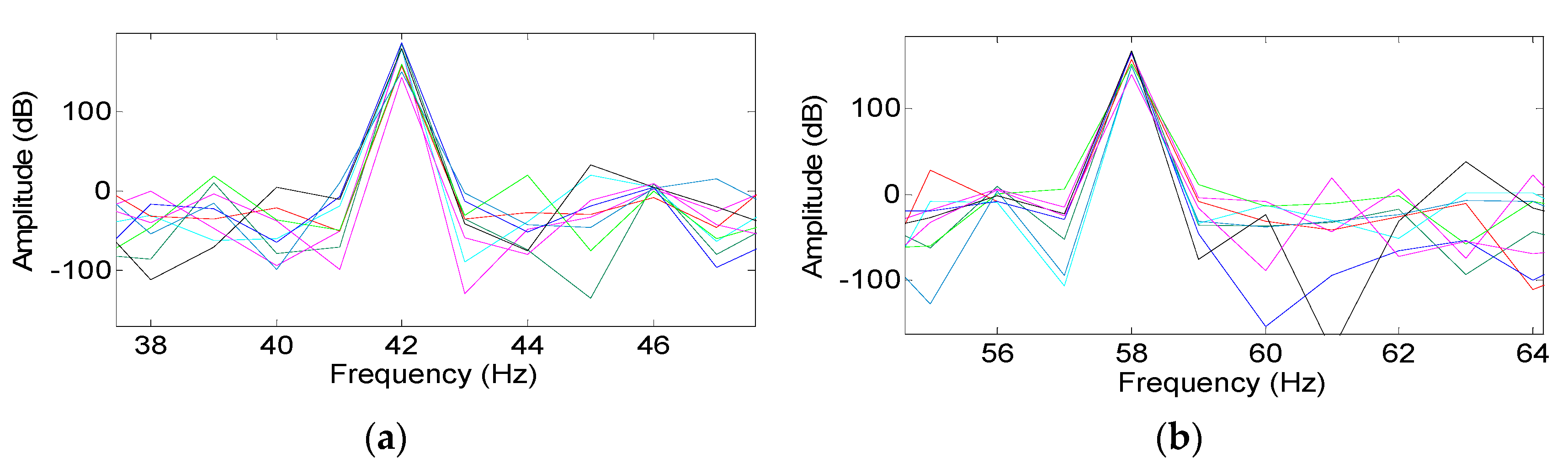
To confirm the overall impact of the nonfunctioning motor on other identified motors, a mirrored and closer look at aberrant frequencies at 42 Hz and 58 Hz shows that the spectrum transforms into a BRB fault peak value, as in following Figure 24.

The respective frequencies at the points 81, 85, and 97 Hz were also identified as abnormal frequencies. Frequency analysis showed no BRB or eccentricity faults. These frequencies were interpreted as errors or noise by the Arduino end node. According to Figure 24, significant frequency points are a source of confusion when attempting to identify a faulty motor because faults tend to mirror themselves across all motors. In order to identify the malfunctioning motor within the network, certain characteristics were compared with one another. Each motor level was assigned a set of four diagnostic features to examine. Amplitude (Amp), Synchronized Speed (SS), and Rotor Slip (RS) are the three components that make up every motor fault. Frequency components all refer to the same thing (of electric current signals). Because of their influence on eccentricity and BRB faults, speed and slip are considered features. Fault diagnosis in multi-motor networks is impossible in the absence of these values. Motor slip is notated in a variety of different ways for each fault in order to provide an estimate of the synchronized speed at each sideband frequency. The severity of a BRB fault can be determined by the amplitude of its frequency components. The learning data-feature sets for all motors are presented in

Table 2. Data set for learning to be used in the training process for several motors in the first case study 1.

Motors	Features				Motor Condition
	SS	RS	Amp	FC
M1	1100	0.33	[44; 50; 56]	[186.5; 370.6; 168.9]	Faulty BRB
M2	1300	0.10	[42; 50; 58]	[180.2; 365; 164.1]	Healthy with some fault symptoms
M3	1280	0.11	[42; 50; 58]	[179.4; 365.2; 160.8]	Healthy with noise
M4	1240	0.12	[42; 50; 58; 97]	[159; 372; 158.5; 102.5]	Healthy
M5	1250	0.11	[42; 50; 58]	[158.6; 372.4; 152]	Healthy
M6	1235	0.10	[42; 50; 58]	[151.3; 364; 150.7]	Healthy
M7	1200	0.09	[42; 50; 58]	[148.1; 365.2; 150.2]	Healthy
M8	1200	0.10	[42; 50; 58;81; 88]	[143.4; 372; 164.1; 90; 43]	Healthy
M9	1210	0.10	[42; 50; 58; 81]	[142.1; 364; 140.4; 75]	Healthy

, which can be used for training and testing to determine each motor’s condition.

From a comparison of the feature ranges, we were able to deduce from Table 2 that the BRB failure had an effect on Motor 1, and since Motors 2 and 3 are on the same sub-bus, they are the ones that are most negatively impacted. Comparing feature ranges made this possible. The BRB fault is not very strong. This is because there is some space in between the motors, which contributes to the separation. As a result of the situation described above, the system mistook these shifts for an undiscovered defect in one of the other motor’s components and interpreted it as a fault. The testing that is done at the microcontroller can tell right away what is wrong with each motor depending on its features and what kind of problem it is based on any changes in how it acts.

5.2. Case Study 2: Differently Defective Motors in Separate Power Buses

The same-sized motors in two different buses were examined for two faults in this second scenario, including a failed test and noise interference from some of the other motors on the same bus. Motor 5 and Motor 9 were chosen from buses 2 and 3 because of their similar sizes. As a result, we were able to examine the effect that defective signals have with other motors in same bus and also motors on these other buses when some other faulty signal passes. In order to increase the level of difficulty, Motor 1, which had the most severe faulty signal, was selected. This was done in order to distinguish among fault signals and locate a possible factor contributing to the malfunctioning of the motor network (Figure 25).

For the purpose of the experiment, the network that is depicted in the following diagram was chosen. In this particular case study, three sensing spots were taken into consideration in order to ascertain the level of fault-signal intensity that was present at various places throughout the network. This was done so that the severity of the fault signal could be observed.

An analysis of the high voltage spectral range produced by all motors is shown in Figure 26 and Figure 27, along with the respective amplitude values. Both figures demonstrate that the mirroring frequency sideband of an eccentricity fault signal does, in fact, appear at the exact same frequency point, but at a different amplitude rate. This is because the amplitude rate is determined by the size of the drive system as well as its distance from Motor 1. Furthermore, the BRB fault spread from Motor 5 to Motor 9, with each motor’s fault signal having a different level of intensity. Table 2 reveals that Motor 1 is not significantly affected by the BRB fault because it is located a considerable distance from other motors that are in need of repair. On the other hand, the amplitude value stands out because of the eccentricity fault.

Figure 28 presents a comparison of the results of the simulation analysis and the experiment in order to verify the reliability of the created prototypes and provide a prognosis of the status of all electric motors within the network. This comparison is made in the context of the analysis of different characteristics of each motor.

6. Discussion

This research utilizes various areas of research in industrial fault identification to come up with an idea of fault multipath propagation inside powerline networks and to show how faulty signals change into healthy electrical impulses while they are travelling in a mapped, distributed powerline network. Within the scope of this study, a methodical approach has been taken to estimate the impact that incorrectly transmitted signals (electric current signals) have on the primary powerline network. It changes the motor behavior of in-network machines’ electric currents. To figure out how different signals could move through a network, an analysis was done to estimate the attenuation aspects of the signals. Faults on multiple paths in a powerline network can be estimated using this analysis. The network’s fault representation is also predicted. Using WSN, different practical experiments have been done to figure out the types of faults and what caused them using multiple point observations. This activity shows how important multiple point observation is and makes traditional methods in MCSA more accurate. It also provides an improved and more efficient way to monitor the behavior of industrial electrical components. Moreover, a plan was made to use the signal processing methodology to change the spectrums and find correlations with the tailored fault symptoms. We show how to use supervised learning to find multiple faults and figure out where they happened in an industrial motor network. Lastly, a complex industrial multi-motor network was modelled and built in the lab to show that bad signals can spread over a powerline network and that wireless nodes can be used to send data for analysis.

A traditional WSN motor network uses Arduino Xbee devices and different-sized motors to create experimental nodes. This experiment showed that faulty indicators can perpetuate through an electricity network and that faults can be identified. All motors were placed in parallel towards the main power, proving that this configuration given a precise working model of a manufacturing multi-motor proposed the concept environment. The different computation and sensor measurement outputs show that real-time data capture is accurate. It has also been demonstrated that data fusion at the end node level and the node coordinator level can produce more complex detection systems as well as more effective fault diagnosis through wireless node-level data transmission.

7. Conclusions and Future Recommendations

This paper suggests a way to find faults by looking at how fault-frequency components move through networks and show them. This method makes it easier to figure out what’s wrong in environments with multiple motors. Simulation data were generated using an optimized industrial model of a distributed-motor network. A systematical approach was necessary because it was important to assess the impact of a fault signal that was propagating. This fault signal was an electric current signal. This demonstrated how the change affects the frequency band behavior of the power line motor features. Signal attenuation factors were analyzed to determine signal paths across a network. This study predicts powerline faults on multiple-path routes. A framework of an experimental wireless sensor network motor network was constructed utilizing Arduino Xbee components and motors of varying sizes. This model showed faulty signal propagation in a power-line network. This architecture offered a trustworthy real-time representation of a modelling environment for industrial multi-motor networks. In this particular setting, each of the motors was linked up to the primary powerline in a parallel configuration. Comparisons between simulation and sensor measurements show close accuracy in real-time data capture. Simulation results differ from sensor measurements, proving this. The development and validation of a sample preparation method for wireless node-level features at the end node level has also been intended to produce more complex detection. In addition to this, decision-level fusion has been implemented at the head node for more accurate fault diagnosis.

In terms of the improvement of fault diagnosis that will take place in the future, additional enhancements could be investigated to enhance overall system operation.

• In this study, the FFT technique was utilized to conduct an analysis of the current spectrum in order to determine the behavior of motor spectrums. More could be learned about fault diagnosis using signal processing techniques like STFT or wavelet transforms that are similar to or even more advanced than those used in fault diagnosis studies. This could improve the reliability and precision of distributed-motor fault diagnosis.
• When attempting to observe the difficult and complicated propagation of faulty signals over powerlines, high-power motors and transformers can be utilized; however, this only serves to further complicate the process of fault diagnosis.
• WSN sensor fusion may require multi-hop mesh networking.
• Hybrid artificial intelligence techniques could be added to the smart fault detection system based on a cloud-edge framework.