
Impact of Producer Service Agglomeration on Carbon Emission Efficiency and Its Mechanism: A Case Study of Urban Agglomeration in the Yangtze River Delta

Abstract
:1. Introduction
2. Literature Review
3. Theoretical Framework
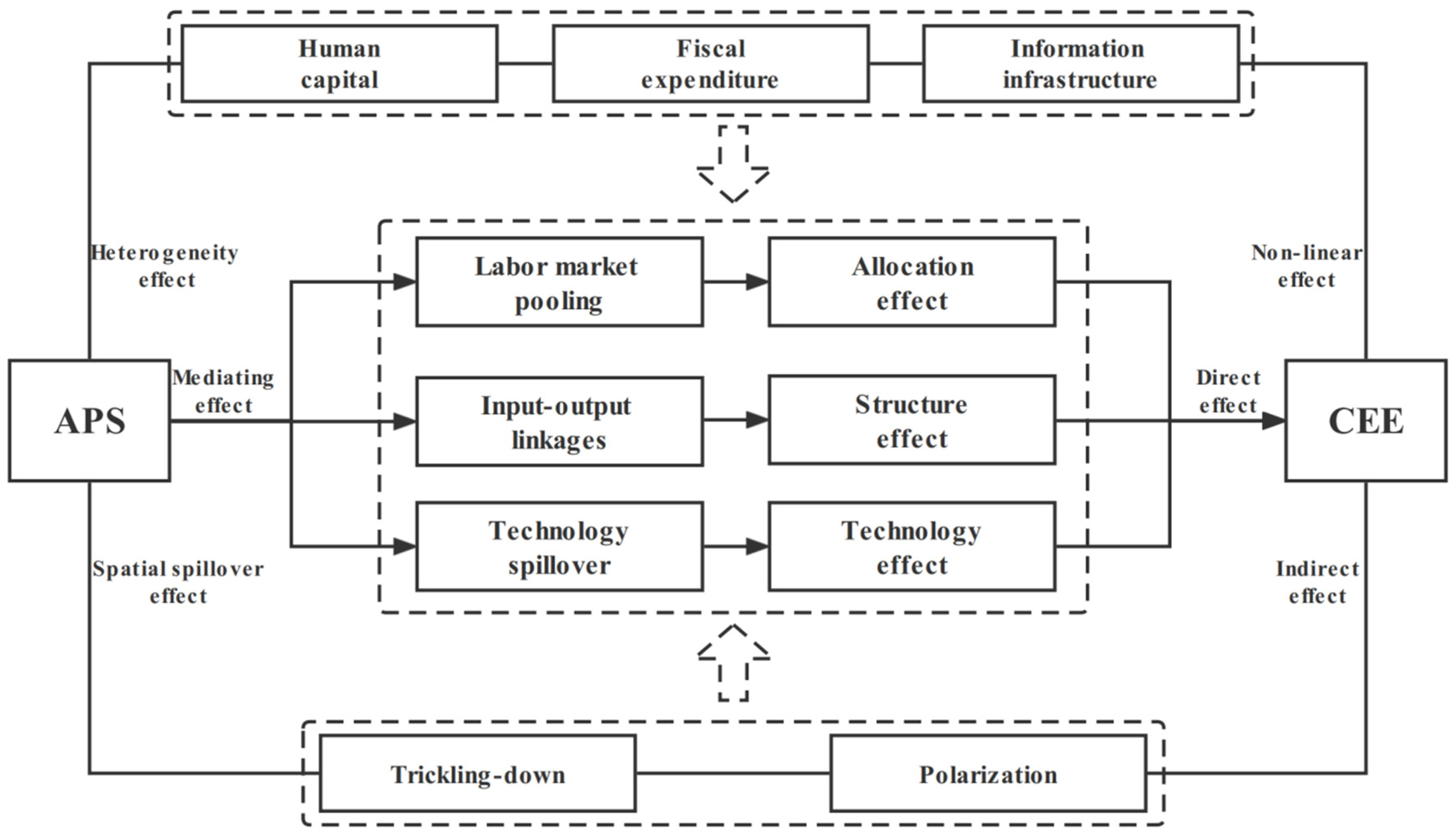
3.1. APS, Intermediary Mechanisms and CEE
3.2. APS, Spatial Spillover and CEE
3.3. APS, Heterogeneity Constraints and CEE
4. Methodology and Data
4.1. Model Setting
4.1.1. Spatial Durbin Model
4.1.2. Mediating Effect Model
4.1.3. Threshold Effect Model
4.2. Variable Selection
4.2.1. Explained Variable
4.2.2. Core Explanatory Variable
4.2.3. Mediating Variables
- (1)
- Allocation effect (RM), which is characterized by the labor misallocation index [57].
- (2)
- Structure effect (IH), which is measured as the ratio of the output value of the tertiary industry to the output value of the secondary industry [58].
- (3)
- Technology effect (GI), which is measured by the number of “green” patent applications per 10,000 people [59].
4.2.4. Threshold Variables
- (1)
- Human factor (HC), we use the number of students in colleges and universities to measure the level of human capital [60].
- (2)
- Financial factor (FS), we use the ratio of fiscal expenditure to regional GDP to measure the scale of fiscal expenditure [61].
- (3)
- Material factor (IT), we use the number of Internet broadband access users to measure the amount of regional information infrastructure [62].
4.2.5. Control Variables
- (1)
- Population factor (P), we use the land area, total population at the end of the year and the location entropy method to measure the population agglomeration.
- (2)
- Affluence factor (A), which is measured by the ratio of regional GDP to the total population at the end of the year.
- (3)
- Environmental regulation (ER), which is measured as the comprehensive utilization rate of industrial solid waste.
- (4)
- Industrial structure (IN), which is the ratio of industrial value added to regional GDP.
- (5)
- Traffic condition (TR), which are measured by the number of buses per capita.
4.2.6. Spatial Weight Matrix
- (1)
- The spatial adjacency weight matrix (W0−1) is defined as follows:
- (2)
- The geographical distance weight matrix (Wd) is defined as follows:where is the distance between two cities calculated from the geographical longitude and latitude.
- (3)
- The economic distance weight matrix (We) is defined as follows:where and are the average per capita GDP of city and from 2005 to 2019.
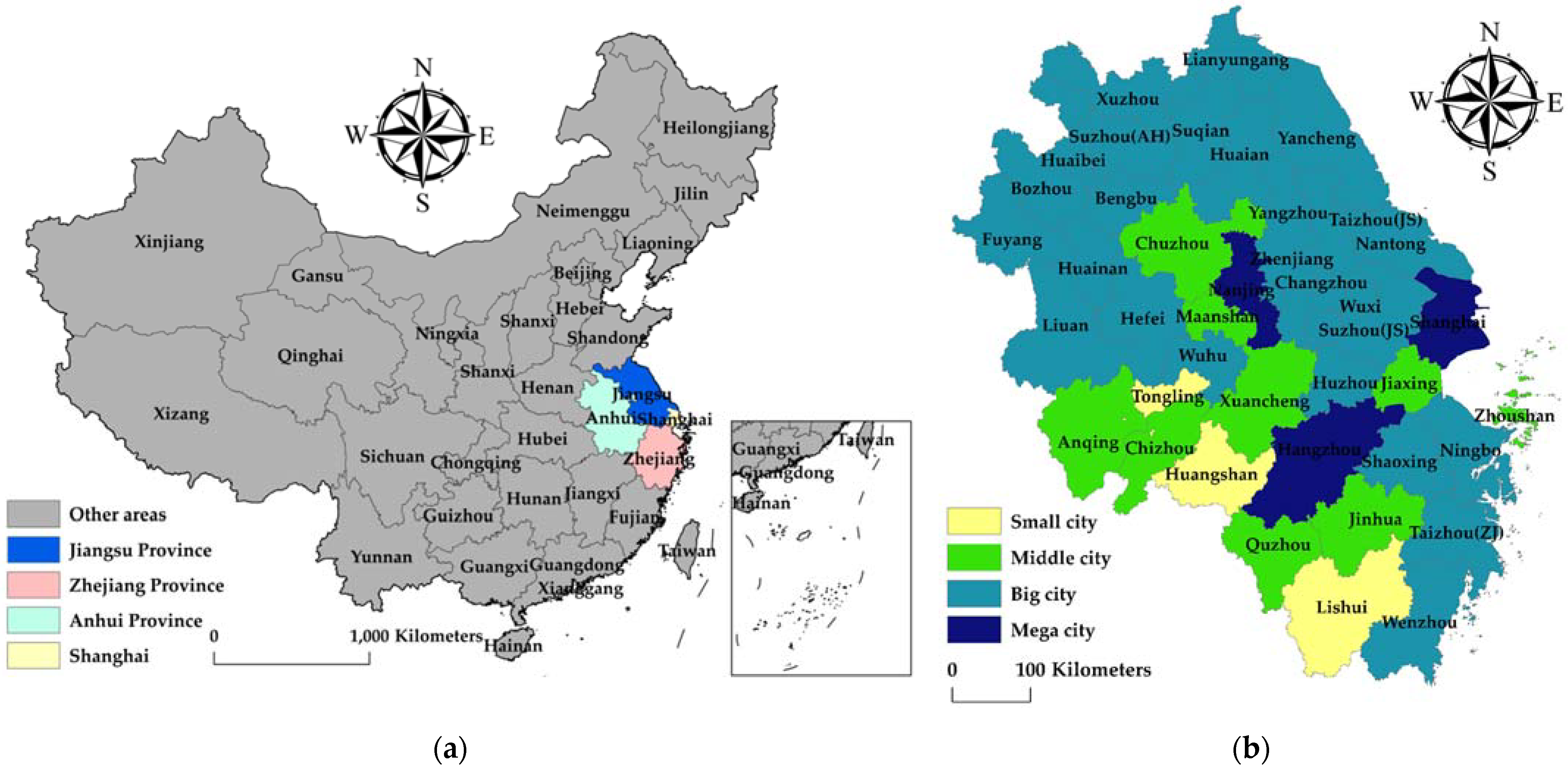
4.3. Data Sources
5. Empirical Analysis
5.1. Spatial Correlation Analysis
5.2. Model Testing and Selection
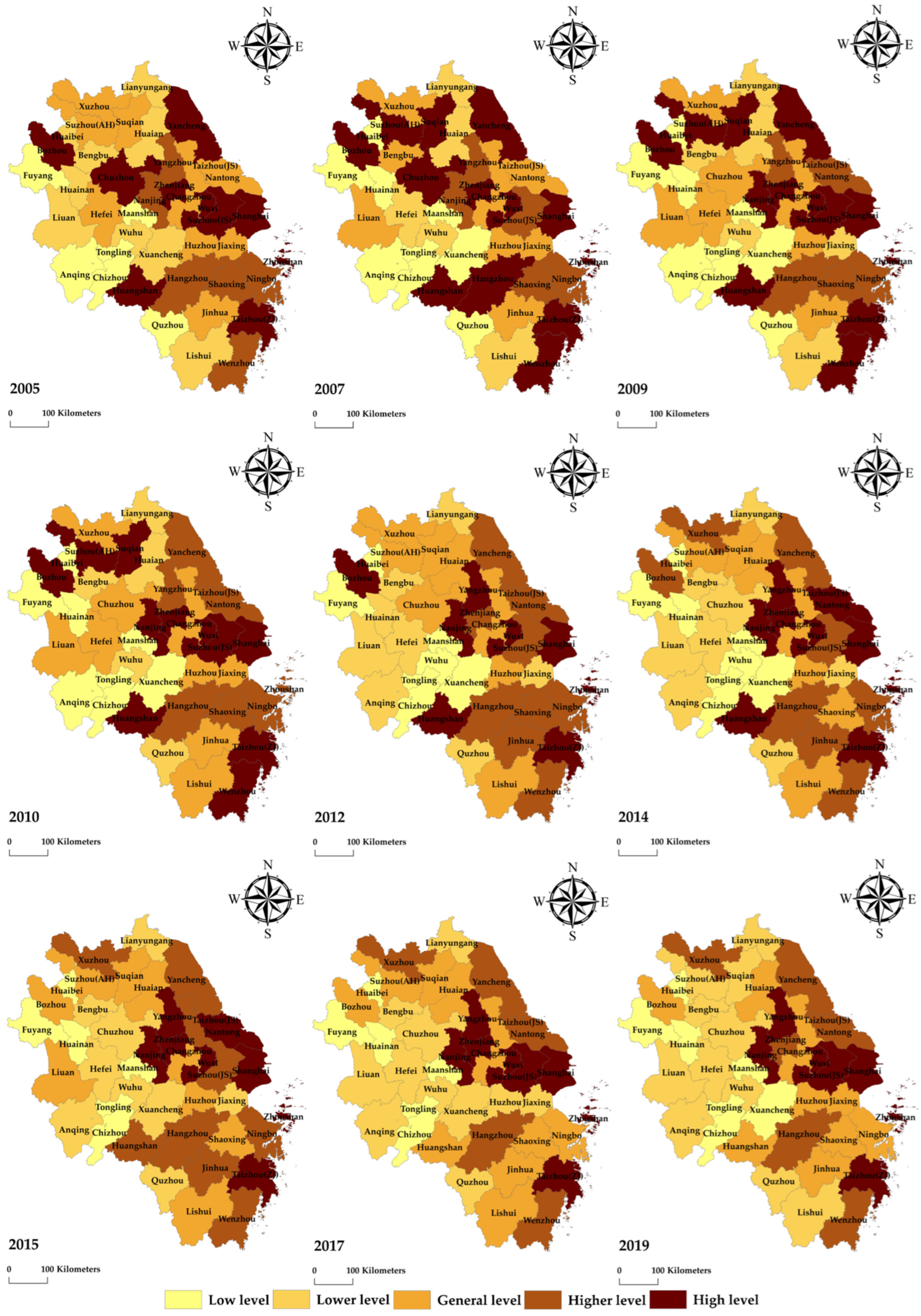
5.3. Spatial Effect Analysis
5.4. Robustness and Endogeneity Tests
6. Discussions
6.1. Mechanistic Analysis
6.2. Heterogeneity Analysis
6.3. Further Discussion Based on Agglomeration Externalities
7. Conclusions and Policy Recommendations
7.1. Conclusions
7.2. Policy Recommendations
7.3. Limitations and Future Directions
Author Contributions
Funding
Institutional Review Board Statement
Informed Consent Statement
Data Availability Statement
Acknowledgments
Conflicts of Interest
References
- Guo, X.; Mu, X.; Ding, Z.; Qin, D. Nonlinear effects and driving mechanism of multidimensional urbanization on PM2.5 concentrations in the Yangtze River Delta. Acta Geogr. Sin. 2021, 76, 1274–1293. [Google Scholar]
- Yuan, H.; Zhang, T.; Feng, Y.; Liu, Y.; Ye, X. Does financial agglomeration promote the green development in China? A spatial spillover perspective. J. Clean. Prod. 2019, 237, 117808. [Google Scholar] [CrossRef]
- Chen, W.; Lan, M.; Sun, W.; Liu, W.; Liu, C. Integrated high-quality development of the Yangtze River Delta: Connotation, current situation and countermeasures. J. Nat. Resour. 2022, 37, 1403–1412. [Google Scholar] [CrossRef]
- Cao, L.; Li, M.; Zhang, L.; Cai, B. Research on Carbon Dioxide Emission Peaking in The Yangtze River Delta Urban Agglomeration. Environ. Eng. 2020, 38, 33–38. [Google Scholar]
- Zhao, J.; Jiang, Q.; Dong, X.; Dong, K.; Jiang, H. How does industrial structure adjustment reduce CO2 emissions? Spatial and mediation effects analysis for China. Energy Econ. 2022, 105, 105704. [Google Scholar] [CrossRef]
- Yin, C.; Huang, N. Spatial Differences in the Development Level of Agricultural Producer Services in China. Asian Agric. Res. 2018, 10, 1–7. [Google Scholar]
- Shao, S.; Tian, Z.; Yang, L. High speed rail and urban service industry agglomeration: Evidence from China’s Yangtze River Delta region. J. Transp. Geogr. 2017, 64, 174–183. [Google Scholar] [CrossRef]
- Mi, K.; Zhuang, R. Producer Services Agglomeration and Carbon Emission Reduction—An Empirical Test Based on Panel Data from China. Sustain. Basel 2022, 14, 3618. [Google Scholar] [CrossRef]
- Zhao, J.; Dong, X.; Dong, K. How does producer services’ agglomeration promote carbon reduction?: The case of China. Econ. Model. 2021, 104, 105624. [Google Scholar] [CrossRef]
- Gao, K.; Yuan, Y. Research on Resource Misallocation Effect of Producer Services Agglomeration from the Perspective of Space. Mod. Econ. Sci. 2020, 42, 108–119. [Google Scholar]
- Li, T.; Han, D.; Feng, S.; Liang, L. Can Industrial Co-Agglomeration between Producer Services and Manufacturing Reduce Carbon Intensity in China? Sustainability 2019, 11, 4024. [Google Scholar] [CrossRef]
- Guo, S.; Pei, Y.; Wu, Y. Research on Industrial Structure Adjustment and Upgrading Effect of the Development of Productive Service Industry. J. Quan. Technol. Econ. 2021, 37, 45–62. [Google Scholar]
- Zhou, X.; Jie, Z.; Li, J. Industrial structural transformation and carbon dioxide emissions in China. Energy Policy 2013, 57, 43–51. [Google Scholar] [CrossRef]
- Cheng, Z.; Li, L.; Liu, J. Industrial structure, technical progress and carbon intensity in China’s provinces. Renew. Sustain. Energy Rev. 2017, 81, 2935–2946. [Google Scholar] [CrossRef]
- Li, L.; Lei, Y.; Wu, S.; He, C.; Chen, J.; Yan, D. Impacts of city size change and industrial structure change on CO2 emissions in Chinese cities. J. Clean. Prod. 2018, 195, 831–838. [Google Scholar] [CrossRef]
- Chen, C.; Sun, Y.; Lan, Q.; Jiang, F. Impacts of industrial agglomeration on pollution and ecological efficiency-A spatial econometric analysis based on a big panel dataset of China’s 259 cities. J. Clean. Prod. 2020, 258, 120721. [Google Scholar] [CrossRef]
- Lu, F.; Wang, Q. Agglomeration of Producer Services and Haze Pollution Control. Soft Sci. 2021, 35, 1–7. [Google Scholar]
- Feng, Y.; Zou, L.; Yuan, H.; Dai, L. The Spatial Spillover Effects and Impact Paths of Financial Agglomeration on Green Development: Evidence from 285 Prefecture-level Cities in China. J. Clean. Prod. 2022, 340, 130816. [Google Scholar] [CrossRef]
- Xie, R.; Yao, S.; Han, F.; Fang, J. Land Finance, Producer Services Agglomeration, and Green Total Factor Productivity. Int. Reg. Sci. Rev. 2019, 42, 550–579. [Google Scholar] [CrossRef]
- Shen, N.; Deng, R.; Wang, Q. Influence of Agglomeration of Manufacturing and the Producer Service Sector on Energy Efficiency. Pol. J. Environ. Stud. 2019, 28, 3401–3418. [Google Scholar] [CrossRef]
- Ren, Y.; Wang, C.; Xu, L.; Yu, C.; Zhang, S. Spatial spillover effect of producer services agglomeration on green economic efficiency: Empirical research based on spatial econometric model. J. Intell. Fuzzy Syst. 2019, 37, 6389–6402. [Google Scholar]
- Huang, F.; Guo, W. Producer Services Agglomeration and Economic Growth Efficiency of the Yangtze River Delta City Cluster from the Perspective of Spatial Spillover. Stat. Res. 2020, 37, 66–79. [Google Scholar]
- Chen, J.; Chen, G.; Huang, J. Study on the Agglomeration of Productive Services and Its Influencing Factors from the Perspective of New Economic Geography: Empirical Data from 222 Cities in China. J. Manag. World 2009, 9, 83–95. [Google Scholar]
- Shen, N. Local Knowledge Spillovers and Productive Service Industry Clustering: Based on City Data Spatial Econometrics. Sci. Sci. Manag. S. T. 2013, 34, 61–69. [Google Scholar]
- Yan, C.; He, H. Agglomeration of Productive Service Industry, Fiscal Decentralization and Prefectural Industrial Ecological Efficiency. Rev. Econ. Manag. 2021, 35, 92–107. [Google Scholar]
- Li, X.; Dai, L.; Mou, S.; Yan, X. Agglomeration of Productive Service Industry and Green Transformation and Upgrading of Manufacturing Industry: Regulatory Role of Information and Communication Technology. J. Southwest Univ. 2022, 48, 83–96. [Google Scholar]
- Romer, P.M. Increasing Returns and Long-Run Growth. J. Polit Econ. 1986, 94, 1002–1037. [Google Scholar] [CrossRef]
- Yuan, H.; Feng, Y.; Yu, Y. Does Manufacturing Agglomeration Promote or Hinder Green Development Performance? Evidence from the Yangtze River Economic Belt. Econ. Geogr. 2022, 42, 121–131. [Google Scholar]
- Yuan, H.; Feng, Y.; Lee, C.; Cen, Y. How does manufacturing agglomeration affect green economic efficiency? Energy Econ. 2020, 92, 104944. [Google Scholar] [CrossRef]
- Yu, Y.; Wei, P.; Gao, X. The Effects of Producer Service Agglomeration on Urban Green Total Factor Productivity—An Analysis Based on 283 Cities in China. Contemp. Econ. Manag. 2021, 43, 54–65. [Google Scholar]
- Han, F.; Qin, J.; Gong, S. Does the Agglomeration of Productive Services Promote the Optimization of Energy Utilization Structure? An Empirical Analysis Based on Dynamic Spatial Durbin Model. J. Nanjing Audit Univ. 2018, 15, 81–93. [Google Scholar]
- Yusuf, S.; Nabeshima, K.; Yamashita, S. Growing Industrial Clusters in Asia: Serendipity and Science. World Bank Publ. 2008, 23, 125–126. [Google Scholar]
- Li, Y.; Shen, B.; Hu, S.; Lin, S. Spatial Effect of Producer Services Agglomeration and Urban Technological Innovation: Empirical Analysis Based on Panel Data of 108 Cities in the Yangtze River Economic Belt. Econ. Geogr. 2021, 41, 65–76. [Google Scholar]
- Hu, S.; Zeng, G.; Cao, X.; Yuan, H.; Chen, B. Does Technological Innovation Promote Green Development? A Case Study of the Yangtze River Economic Belt in China. Int. J. Environ. Res. Public Health 2021, 18, 6111. [Google Scholar] [CrossRef] [PubMed]
- Yuan, H.; Liu, Y.; Feng, Y. How does Financial Agglomeration Affect Green Development Efficiency? Empirical Analysis SPDM and PTR Models Considering Spatio-temporal Double Fixation. Chin. J. Manag. Sci. 2019, 27, 61–75. [Google Scholar]
- Luo, C.; Zhu, P.; Zhang, C.; Chen, W. Does Producer Services Agglomeration Promote Urban Green Innovation? Froom the Perspective of “Local-Neighborhood” Effect. J. Southwest Univ. 2022, 48, 97–112. [Google Scholar]
- Han, F.; Xie, R. Does the Agglomeration of Producer Services Reduce Carbon Emissions? J. Quant. Tech. Econ. 2017, 34, 40–58. [Google Scholar]
- Shen, W.; Chai, Z.; Zhang, S. The Effect of Industrial Synergistic Agglomeration on Industrial Pollution Reduction: Based on the Yangtze River Delta Urban Agglomeration. East China Econ. Manag. 2020, 34, 84–94. [Google Scholar]
- Yang, H.; Zhang, F.; He, Y. Exploring the effect of producer services and manufacturing industrial co-agglomeration on the ecological environment pollution control in China. Environ. Dev. Sustain. 2021, 23, 16119–16144. [Google Scholar] [CrossRef]
- Akinci, M. Inequality and economic growth: Trickle-down effect revisited. Dev. Policy Rev. 2017, 36, 1–24. [Google Scholar] [CrossRef]
- Gil-Alana, L.A.; Kare, M.; Priklas-Drueta, R. Measuring inequality persistence in OECD 1963–2008 using fractional integration and cointegration. Q. Rev. Econ. Financ. 2019, 72, 65–72. [Google Scholar] [CrossRef]
- Yu, Y.; Gao, X. Why People Flow to Big Cities: A Review of Urban Agglomeration and Labor Migration. East China Econ. Manag. 2017, 31, 82–87. [Google Scholar]
- Yuan, H.; Liu, Y. Financial agglomeration and green development efficiency: A two-dimensional perspective based on level and efficiency. Sci. Res. Manag. 2019, 40, 126–143. [Google Scholar]
- Han, F.; Yang, L. How Does the Agglomeration of Producer Services Promote the Upgrading of Manufacturing Structure?: An Integrated Framework of Agglomeration Economies and Schumpeter’s Endogenous Growth Theory. J. Manag. World 2020, 36, 72–94. [Google Scholar]
- Huo, P. Research on the Dynamic Evolution and Driving Factors of Spatial Agglomeration of Knowledge-intensive Services. Resour. Environ. Yangtze Basin 2022, 31, 770–780. [Google Scholar]
- Wang, K.; Zhao, B.; Ding, L.; Miao, Z. Government intervention, market development, and pollution emission efficiency: Evidence from China. Sci. Total Environ. 2020, 757, 143738. [Google Scholar] [CrossRef] [PubMed]
- Panayides, A.; Kern, C.R. Kern Information Technology and the Future of Cities: An Alternative Analysis. Urban Stud. 2005, 42, 163–167. [Google Scholar] [CrossRef]
- Nguyen, C.P.; Schinckus, C.; Dinh, T.S.; Ling, F. The determinants of the Energy Consumption: A Shadow Economy-based perspective. Energy 2021, 225, 120210. [Google Scholar]
- Han, F.; Xie, R.; Lu, Y.; Fang, J.; Liu, Y. The effects of urban agglomeration economies on carbon emissions: Evidence from Chinese cities. J. Clean. Prod. 2018, 172, 1096–1110. [Google Scholar] [CrossRef]
- Feng, Y.; Wang, X.; Liang, Z.; Hu, S.; Wu, G. Effects of Emission Trading System on Green Total Factor Productivity in China: Empirical Evidence from a Quasi-natural Experiment. J. Clean. Prod. 2021, 294, 126262. [Google Scholar] [CrossRef]
- Chen, Y.; Lee, C.C. Does technological innovation reduce CO2 emissions? Cross-country evidence. J. Clean. Prod. 2020, 263, 121550. [Google Scholar] [CrossRef]
- Hansen, B.E. Threshold effects in non-dynamic panels: Estimation, testing, and inference. J. Econom. 1999, 93, 345–368. [Google Scholar] [CrossRef]
- Tone, K. A slacks-based measure of efficiency in data envelopment analysis. Eur. J. Oper. Res. 2001, 130, 498–509. [Google Scholar] [CrossRef]
- Guo, P.; Liang, D. Does the low-carbon pilot policy improve the efficiency of urban carbon emissions: Quasinatural experimental research based on low-carbon pilot cities. J. Nat. Resour. 2022, 37, 1876–1892. [Google Scholar] [CrossRef]
- Zheng, Q.; Lin, B. Impact of industrial agglomeration on energy efficiency in China’s paper industry. J. Clean. Prod. 2018, 184, 1072–1080. [Google Scholar] [CrossRef]
- Yu, B. The Agglomeration of Producer Services and Improve Energy Efficiency. Stat. Res. 2018, 35, 30–40. [Google Scholar]
- Chen, Y.; Hu, W. Distortions, Misallocation and Losses: Theory and Application. China Econ. Q. 2011, 10, 1401–1422. [Google Scholar]
- Wang, K.; Wu, M.; Sun, Y.; Shi, X.; Sun, A.; Zhang, P. Resource abundance, industrial structure, and regional carbon emissions efficiency in China. Resour. Policy 2019, 60, 203–214. [Google Scholar] [CrossRef]
- Liu, Y.; Zhu, J.; Li, E.Y.; Meng, Z.; Song, Y. Environmental regulation, green technological innovation, and eco-efficiency: The case of Yangtze river economic belt in China. Technol. Ther. Soc. 2020, 155, 119993. [Google Scholar] [CrossRef]
- Feng, Y.; Wang, X.; Du, W.; Liu, J.; Li, Y. Spatiotemporal characteristics and driving forces of urban sprawl in China during 2003–2017. J. Clean. Prod. 2019, 241, 118061. [Google Scholar] [CrossRef]
- Feng, Y.; Wang, X. Effects of urban sprawl on haze pollution in China based on dynamic spatial Durbin model during 2003–2016. J. Clean. Prod. 2019, 242, 118368. [Google Scholar] [CrossRef]
- Feng, Y.; He, F. The effect of environmental information disclosure on environmental quality: Evidence from Chinese cities. J. Clean. Prod. 2020, 276, 124027. [Google Scholar] [CrossRef]
- Feng, Y.; Wang, X.; Du, W.; Wu, H.; Wang, J. Effects of environmental regulation and FDI on urban innovation in China: A spatial Durbin econometric analysis. J. Clean. Prod. 2019, 235, 210–224. [Google Scholar] [CrossRef]
- Yuan, H.; Zhang, T.; Hu, K.; Feng, Y.; Feng, C.; Jia, P. Influences and transmission mechanisms of financial agglomeration on environmental pollution. J. Environ. Manag. 2021, 303, 114136. [Google Scholar] [CrossRef]
- LeSage, J.P.; Pace, R.K. The Biggest Myth in Spatial Econometrics. Econometrics 2014, 2, 217–249. [Google Scholar] [CrossRef]
- Ren, G.; Wan, J.; Liu, J.; Yu, D. Spatial and temporal correlation analysis of wind power between different provinces in China. Energy 2020, 191, 116514. [Google Scholar] [CrossRef]
- Lesage, J.; Pace, R.K. Spatial Econometrics. Book Chapters 2010, 1, 245–260. [Google Scholar]
- Han, F.; Xie, R.; Lai, M. Traffic density, congestion externalities, and urbanization in China. Spat. Econ. Anal. 2018, 13, 400–421. [Google Scholar] [CrossRef]
- Zeng, Y.; Han, F.; Liu, J. Does the Agglomeration of Producer Services Promote the Quality of Urban Economic Growth? J. Quan. Technol. Econ. 2019, 36, 83–100. [Google Scholar]
- Zhang, H. Producer Services Agglomeration and Urban Economic Performance: Analysis from Industrial and Regional Heterogeneity Perspectives. J. Financ. Econ. 2015, 41, 67–77. [Google Scholar]


| Indicator Type | Primary Indicators | Secondary Indicators |
|---|---|---|
| Input indicators | Capital input | Fixed capital stock |
| Labor input | Number of employed people at the end of the year | |
| Energy input | Electricity consumption of the whole society Natural gas Liquefied petroleum gas | |
| Output types | Desirable output | GDP |
| Undesirable output | Carbon emissions |
| Type | Variables | Observation | Mean | Std.Dev | Min | Max |
|---|---|---|---|---|---|---|
| Explained variable | 615 | 0.7177 | 0.2350 | 0.2390 | 1.4147 | |
| Core explanatory variable | 615 | 0.8228 | 0.2926 | 0.2905 | 2.1089 | |
| 615 | 1.3941 | 0.6051 | 0.4213 | 3.9781 | ||
| 615 | 14.0883 | 6.3941 | 4.2105 | 76.1037 | ||
| 615 | 31,189.9900 | 24,331.8900 | 5714.1310 | 205,457.0000 | ||
| Mediating variable | 615 | 0.3678 | 0.3128 | 0.0003 | 1.5569 | |
| 615 | 0.8918 | 0.3001 | 0.3127 | 2.6946 | ||
| 615 | 2.1222 | 3.2829 | 0.0000 | 22.4099 | ||
| Threshold variable | 615 | 10.1496 | 15.0685 | 0.1700 | 87.7894 | |
| 615 | 0.1489 | 0.0814 | 0.0553 | 1.4852 | ||
| 615 | 2166.8400 | 2358.7660 | 70.2454 | 36,634.7600 | ||
| Control variable | 615 | 2.5762 | 1.3513 | 0.5449 | 10.2922 | |
| 615 | 43,956.7400 | 37,280.4900 | 2831.1020 | 204,350.1000 | ||
| 615 | 92.2484 | 8.6617 | 40.0700 | 100.0000 | ||
| 615 | 0.4210 | 0.0886 | 0.1687 | 0.6966 | ||
| 615 | 7.9038 | 4.4964 | 0.4330 | 25.0724 | ||
| Spatial weight matrix | Matrix element in which two places are adjacent is 1, otherwise is 0. | |||||
| ) | The elements of the matrix are the square of the inverse of the distance between the centers of mass of the two places. | |||||
| ) | The matrix element is the square of the inverse of the difference between the annual average GDP per capita of the two places. | |||||
| Year | Moran’s I | Geary’s C | ||
|---|---|---|---|---|
| Statistic Value | p-Value | Statistic Value | p-Value | |
| 2005 | 0.171 ** | 0.027 | 0.779 ** | 0.015 |
| 2006 | 0.064 | 0.193 | 0.901 | 0.165 |
| 2007 | 0.054 | 0.219 | 0.907 | 0.179 |
| 2008 | 0.059 | 0.206 | 0.910 | 0.188 |
| 2009 | 0.072 | 0.169 | 0.885 | 0.128 |
| 2010 | 0.103 | 0.104 | 0.868 * | 0.097 |
| 2011 | 0.183 ** | 0.020 | 0.775 ** | 0.014 |
| 2012 | 0.267 *** | 0.002 | 0.679 *** | 0.001 |
| 2013 | 0.381 *** | 0.000 | 0.573 *** | 0.000 |
| 2014 | 0.322 *** | 0.000 | 0.623 *** | 0.000 |
| 2015 | 0.393 *** | 0.000 | 0.556 *** | 0.000 |
| 2016 | 0.370 *** | 0.000 | 0.585 *** | 0.000 |
| 2017 | 0.399 *** | 0.000 | 0.559 *** | 0.000 |
| 2018 | 0.400 *** | 0.000 | 0.556 *** | 0.000 |
| 2019 | 0.412 *** | 0.000 | 0.550 *** | 0.000 |
| Contents | Methods | Statistic Value | p-Value |
|---|---|---|---|
| Panel spatial correlation test | Moran’s I | 3.395 *** | 0.001 |
| SLM model and SEM model test | LM-lag test | 213.182 *** | 0.000 |
| R-LM-lag test | 25.488 *** | 0.000 | |
| LM-err test | 215.023 *** | 0.000 | |
| R-LM-err test | 27.329 *** | 0.000 | |
| Simplified test of SDM model | Wald-lag test | 77.95 *** | 0.000 |
| LR-lag test | 73.98 *** | 0.000 | |
| Wald-err test | 80.22 *** | 0.000 | |
| LR-err test | 74.71 *** | 0.000 | |
| Hausman test of SDM model | Hausman test | 293.85 *** | 0.000 |
| Type | Variable | OLS | SEM | SLM | SDM |
|---|---|---|---|---|---|
| 0.0724 (1.20) | −0.0082 (−0.15) | 0.0309 (0.56) | 0.1086 ** (2.01) | ||
| 0.1768 *** (2.93) | 0.0839 (1.56) | 0.1233 ** (2.35) | 0.1971 *** (3.89) | ||
| 0.2902 ** (2.43) | 0.2127 ** (2.00) | 0.2301 ** (2.19) | 0.1867 * (1.83) | ||
| 0.3391 *** (4.78) | 0.3421 *** (6.07) | 0.3281 *** (5.87) | 0.3372 *** (6.18) | ||
| −0.0013 (−0.02) | −0.0253 (−0.51) | −0.0100 (−0.20) | −0.0210 (−0.44) | ||
| −0.4383 *** (−7.36) | −0.4450 *** (−9.27) | −0.3947 *** (−8.89) | −0.4099 *** (−7.68) | ||
| −0.0520 ** (−2.48) | −0.0567 *** (−3.62) | −0.0609 *** (−3.79) | −0.0486 *** (−3.00) | ||
| 0.8730 *** (7.08) | |||||
| 0.9191 *** (7.80) | |||||
| 0.2483 (1.27) | |||||
| 0.0913 (0.78) | |||||
| 0.2107 ** (2.00) | |||||
| 0.1999 ** (2.51) | |||||
| 0.0362 (1.03) | |||||
| City FE | YES | YES | YES | YES | |
| Year FE | YES | YES | YES | YES | |
| Observation | 615 | 615 | 615 | 615 | |
| Direct effect | 0.0724 (1.20) | −0.0082 (−0.15) | 0.0332 (0.58) | 0.1359 ** (2.49) | |
| 0.1768 *** (2.93) | 0.0839 (1.56) | 0.1251 ** (2.37) | 0.2244 *** (4.57) | ||
| 0.2902 ** (2.43) | 0.2127 ** (2.00) | 0.2420 ** (2.39) | 0.2032 ** (2.09) | ||
| 0.3391 *** (4.78) | 0.3421 *** (6.07) | 0.3304 *** (6.24) | 0.3396 *** (6.62) | ||
| −0.0013 (−0.02) | −0.0253 (−0.51) | −0.0093 (−0.19) | −0.0140 (−0.30) | ||
| −0.4383 *** (−7.36) | −0.4450 *** (−9.27) | −0.3969 *** (−9.01) | −0.4030 *** (−7.77) | ||
| −0.0520 ** (−2.48) | −0.0567 *** (−3.62) | −0.0619 *** (−3.61) | −0.0479 *** (−2.76) | ||
| Indirect effect | 0.0080 (0.52) | 0.9864 *** (7.46) | |||
| 0.0318 ** (2.10) | 1.0571 *** (8.77) | ||||
| 0.0624 ** (2.09) | 0.3121 (1.47) | ||||
| 0.0860 *** (3.39) | 0.1415 (1.08) | ||||
| −0.0030 (−0.22) | 0.2372 * (1.95) | ||||
| −0.1032 *** (−3.77) | 0.1614 ** (2.13) | ||||
| −0.0163 ** (−2.45) | 0.0360 (0.87) |
| Type | Variable | Replace the Spatial Weight Matrix | Substitution of Explained Variable | Substitution of Core Explanatory Variable | Excluding Regression Samples | Instrumental Variable Regression | |||||
|---|---|---|---|---|---|---|---|---|---|---|---|
| (1) | (2) | (3) | (4) | (5) | (6) | (7) | (8) | (9) | (10) | ||
| Direct effect | 0.0743 (1.29) | 0.0489 (0.90) | −0.1317 ** (−2.47) | 0.0600 (1.48) | 0.0985 ** (2.17) | −0.2924 *** (−5.69) | 0.0306 (0.52) | 0.0738 (1.33) | 0.1344 (1.10) | 0.1659 ** (2.26) | |
| 0.1642 *** (3.16) | 0.1760 *** (3.58) | −0.0907 * (−1.87) | 0.0736 ** (2.02) | 0.1956 *** (4.42) | 0.0659*** (7.93) | 0.1248 ** (2.33) | 0.1937 *** (3.80) | 0.2264 * (1.85) | 0.3174 *** (4.03) | ||
| Indirect effect | 0.2669 (1.60) | 0.0595 (0.87) | −0.3590 ** (−2.35) | 0.2440 *** (2.64) | 0.7628 *** (6.32) | −0.0687 (−0.70) | 0.6979 *** (5.22) | 0.9173 *** (7.14) | 0.9195 *** (3.50) | 0.9599 *** (7.45) | |
| 0.3994 *** (2.91) | 0.2605 *** (4.37) | −0.4786 *** (−3.28) | 0.3327 *** (3.88) | 0.8256 *** (7.37) | 0.0330 ** (2.17) | 0.8160 *** (6.55) | 1.0255 *** (8.56) | 0.9950 *** (4.26) | 1.0085 *** (8.42) | ||
| Kleibergen-Paap rk LM statistic | 39.929 [0.0000] | ||||||||||
| Kleibergen-Paap rk Wald F statistic | 46.966 {7.03} | ||||||||||
| Control | YES | YES | YES | YES | YES | YES | YES | YES | YES | YES | |
| City FE | YES | YES | YES | YES | YES | YES | YES | YES | YES | YES | |
| Year FE | YES | YES | YES | YES | YES | YES | YES | YES | YES | YES | |
| Observation | 615 | 615 | 615 | 615 | 615 | 615 | 600 | 615 | 615 | 615 | |
| Variable | Allocative Effect | Structure Effect | Technology Effect | |||
|---|---|---|---|---|---|---|
(1) | (2) | (3) | (4) | (5) | (6) | |
| 0.4300 *** (4.38) | 0.0968 (1.50) | 0.1901 *** (5.07) | 0.0317 (0.51) | 3.3756 *** (3.46) | 0.0113 (0.19) | |
| −0.2056 * (−1.74) | 0.1652 *** (2.77) | 0.1747 *** (4.74) | 0.1394 ** (2.32) | 1.8315 ** (2.11) | 0.1437 ** (2.43) | |
| −0.0568 * (−1.92) | ||||||
| 0.2141 ** (1.99) | ||||||
| 0.0181 *** (6.47) | ||||||
| Control | YES | YES | YES | YES | YES | YES |
| City FE | YES | YES | YES | YES | YES | YES |
| Year FE | YES | YES | YES | YES | YES | YES |
| Observation | 615 | 615 | 615 | 615 | 615 | 615 |
| Panel A: Threshold Effect Test | |||||||
|---|---|---|---|---|---|---|---|
| F-value | p-value | BS | 1% | 5% | 10% | Threshold value | |
| Single threshold | 41.81 | 0.0667 | 300 | 57.6858 | 44.3625 | 35.2492 | 24.3788 |
| Double threshold | 11.73 | 0.7800 | 300 | 50.7724 | 37.9895 | 32.4624 | 1.6022 |
| Triple threshold | 23.15 | 0.4633 | 300 | 59.6886 | 49.0570 | 42.6643 | 0.9722 |
| F-value | p-value | BS | 1% | 5% | 10% | Threshold value | |
| Single threshold | 64.76 | 0.0067 | 300 | 61.5269 | 41.3541 | 36.0535 | 0.2086 |
| Double threshold | 37.54 | 0.0533 | 300 | 45.1751 | 37.5892 | 32.5775 | 0.1505 |
| Triple threshold | 8.59 | 0.8400 | 300 | 42.0390 | 33.1135 | 28.2986 | 0.1239 |
| F-value | p-value | BS | 1% | 5% | 10% | Threshold value | |
| Single threshold | 31.67 | 0.0533 | 300 | 52.5238 | 32.1567 | 28.1236 | 394.3066 |
| Double threshold | 15.95 | 0.3033 | 300 | 39.2158 | 28.8934 | 22.8907 | 1402.0537 |
| Triple threshold | 9.13 | 0.5933 | 300 | 42.3442 | 28.8167 | 23.9055 | 6961.6519 |
| Panel B: Estimation Results of Threshold Effect | |||||||
| Variable | (1) | (2) | (3) | ||||
| −0.2055 *** (−5.39) | |||||||
| 0.9562 *** (5.28) | |||||||
| −0.2425 *** (−6.58) | |||||||
| 0.0037 (0.08) | |||||||
| 0.3754 *** (5.72) | |||||||
| −0.5236 *** (−6.81) | |||||||
| −0.1447 *** (−3.84) | |||||||
| Control | YES | YES | YES | ||||
| Observation | 615 | 615 | 615 | ||||
| Panel C: Threshold Interval Division | |||||||
| Threshold interval | City (in 2005) | City (in 2019) | |||||
| Hefei, Anqing, Bengbu, Chizhou, Chuzhou, Fuyang, Huaibei, Huainan, Huangshan, Liuan, Maanshan, Suzhou(AH), Tongling, Wuhu, Xuancheng, Bozhou, Changzhou, Huaian, Lianyungang, Nantong, Suzhou(JS), Suqian, Taizhou(JS), Wuxi, Xuzhou, Yancheng, Yangzhou, Zhenjiang, Huzhou, Jiaxing, Jinhua, Lishui, Ningbo, Shaoxing, Taizhou(ZJ), Wenzhou, Zhoushan, Quzhou (Total 38 cities) | Anqing, Bengbu, Chizhou, Chuzhou, Fuyang, Huaibei, Huainan, Huangshan, Liuan, Maanshan, Suzhou(AH), Tongling, Wuhu, Xuancheng, Bozhou, Changzhou, Huaian, Lianyungang, Nantong, Suzhou(JS), Suqian, Taizhou(JS), Wuxi, Xuzhou, Yancheng, Yangzhou, Zhenjiang, Huzhou, Jiaxing, Jinhua, Lishui, Ningbo, Shaoxing, Taizhou(ZJ), Wenzhou, Zhoushan, Quzhou (Total 37 cities) | ||||||
| Nanjing, Shanghai, Hangzhou (Total 3 cities) | Hefei, Nanjing, Shanghai, Hangzhou (Total 4 cities) | ||||||
| Hefei, Anqing, Bengbu, Chizhou, Chuzhou, Fuyang, Huaibei, Huainan, Huangshan, Liuan, Maanshan, Suzhou(AH), Tongling, Wuhu, Xuancheng, Bozhou, Nanjing, Changzhou, Huaian, Lianyungang, Nantong, Suzhou(JS), Suqian, Taizhou(JS), Wuxi, Xuzhou, Yancheng, Yangzhou, Zhenjiang, Hangzhou, Huzhou, Jiaxing, Jinhua, Lishui, Ningbo, Shaoxing, Taizhou(ZJ), Wenzhou, Zhoushan, Quzhou (Total 40 cities) | Hefei, Maanshan, Wuhu, Changzhou, Huaian, Lianyungang, Nanjing, Nantong, Suzhou(JS), Taizhou(JS), Wuxi, Xuzhou, Yangzhou, Zhenjiang, Hangzhou, Huzhou, Jiaxing, Jinhua, Ningbo, Shaoxing, Taizhou(ZJ) (Total 21 cities) | ||||||
| Shanghai (Total 1 cities) | Anqing, Bengbu, Chizhou, Chuzhou, Huaibei, Huainan, Tongling, Suqian, Yancheng, Wenzhou (Total 10 cities) | ||||||
| None | Fuyang, Huangshan, Liuan, Suzhou(AH), Xuancheng, Bozhou, Shanghai, Lishui, Zhoushan, Quzhou (Total 10 cities) | ||||||
| Anqing, Chizhou, Chuzhou, Fuyang, Huaibei, Huainan, Huangshan, Liuan, Suzhou(AH), Tongling, Xuancheng, Bozhou, Huaian, Lianyungang, Nantong, Suqian, Xuzhou, Yancheng (Total 18 cities) | None | ||||||
| Hefei, Bengbu, Maanshan, Wuhu, Nanjing, Changzhou, Suzhou(JS), Taizhou(JS), Wuxi, Yangzhou, Zhenjiang, Shanghai, Hangzhou, Huzhou, Jiaxing, Jinhua, Lishui, Ningbo, Shaoxing, Taizhou(ZJ), Wenzhou, Zhoushan, Quzhou (Total 23 cities) | Hefei, Anqing, Bengbu, Chizhou, Chuzhou, Fuyang, Huaibei, Huainan, Huangshan, Liuan, Maanshan, Suzhou(AH), Tongling, Wuhu, Xuancheng, Bozhou, Nanjing, Changzhou, Huaian, Lianyungang, Nantong, Suzhou(JS), Suqian, Taizhou(JS), Wuxi, Xuzhou, Yancheng, Yangzhou, Zhenjiang, Shanghai, Hangzhou, Huzhou, Jiaxing, Jinhua, Lishui, Ningbo, Shaoxing, Taizhou(ZJ), Wenzhou, Zhoushan, Quzhou (Total 41 cities) | ||||||
| Variable | MAR | Jacobs | Porter | ||||||
|---|---|---|---|---|---|---|---|---|---|
| Direct Effect | Indirect Effect | Total Effect | Direct Effect | Indirect Effect | Total Effect | Direct Effect | Indirect Effect | Total Effect | |
| −0.0824 *** (−3.51) | −0.1559 *** (−2.85) | −0.2383 *** (−4.00) | −0.6598 *** (−5.63) | −0.3242 (−1.15) | −0.9840 *** (−3.17) | −2.4057 *** (−9.54) | −1.4358 ** (−2.57) | −3.8415 *** (−6.13) | |
| 0.1571 *** (6.27) | 0.2454 *** (4.02) | 0.4025 *** (5.82) | 0.1038 *** (4.92) | 0.0248 (0.47) | 0.1287 ** (2.22) | 0.1140 *** (9.43) | 0.0767 *** (2.85) | 0.1906 *** (6.40) | |
| Control | YES | YES | YES | ||||||
| City FE | YES | YES | YES | ||||||
| Year FE | YES | YES | YES | ||||||
| Observation | 615 | 615 | 615 | ||||||
Publisher’s Note: MDPI stays neutral with regard to jurisdictional claims in published maps and institutional affiliations. |
© 2022 by the authors. Licensee MDPI, Basel, Switzerland. This article is an open access article distributed under the terms and conditions of the Creative Commons Attribution (CC BY) license (https://creativecommons.org/licenses/by/4.0/).
Share and Cite
Ma, Y.; Yao, Q. Impact of Producer Service Agglomeration on Carbon Emission Efficiency and Its Mechanism: A Case Study of Urban Agglomeration in the Yangtze River Delta. Sustainability 2022, 14, 10053. https://doi.org/10.3390/su141610053
Ma Y, Yao Q. Impact of Producer Service Agglomeration on Carbon Emission Efficiency and Its Mechanism: A Case Study of Urban Agglomeration in the Yangtze River Delta. Sustainability. 2022; 14(16):10053. https://doi.org/10.3390/su141610053
Chicago/Turabian StyleMa, Yaoshan, and Qingyu Yao. 2022. "Impact of Producer Service Agglomeration on Carbon Emission Efficiency and Its Mechanism: A Case Study of Urban Agglomeration in the Yangtze River Delta" Sustainability 14, no. 16: 10053. https://doi.org/10.3390/su141610053
APA StyleMa, Y., & Yao, Q. (2022). Impact of Producer Service Agglomeration on Carbon Emission Efficiency and Its Mechanism: A Case Study of Urban Agglomeration in the Yangtze River Delta. Sustainability, 14(16), 10053. https://doi.org/10.3390/su141610053