
Predicting Frost Depth of Soils in South Korea Using Machine Learning Techniques


Abstract
:1. Introduction
2. Dataset
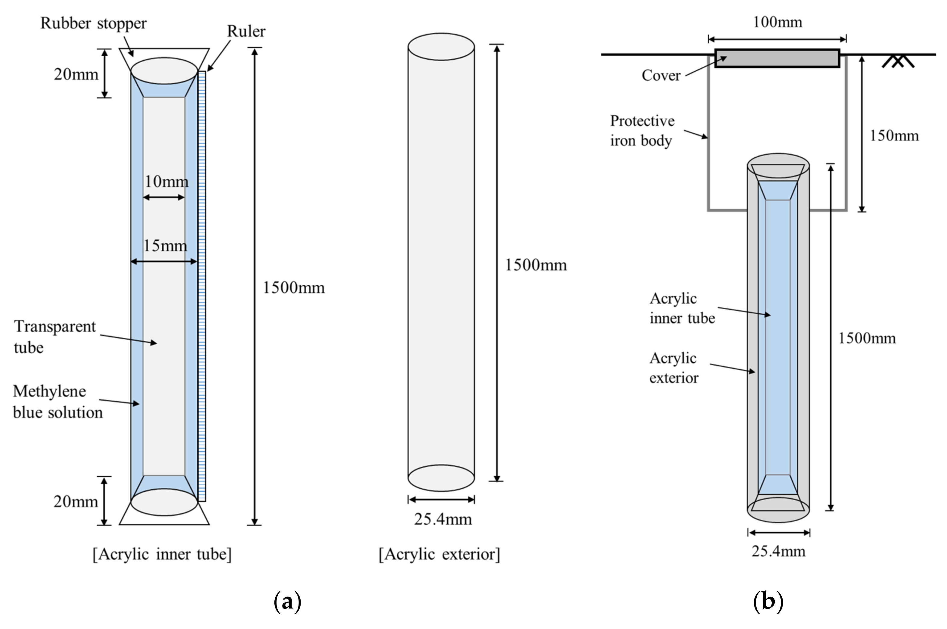
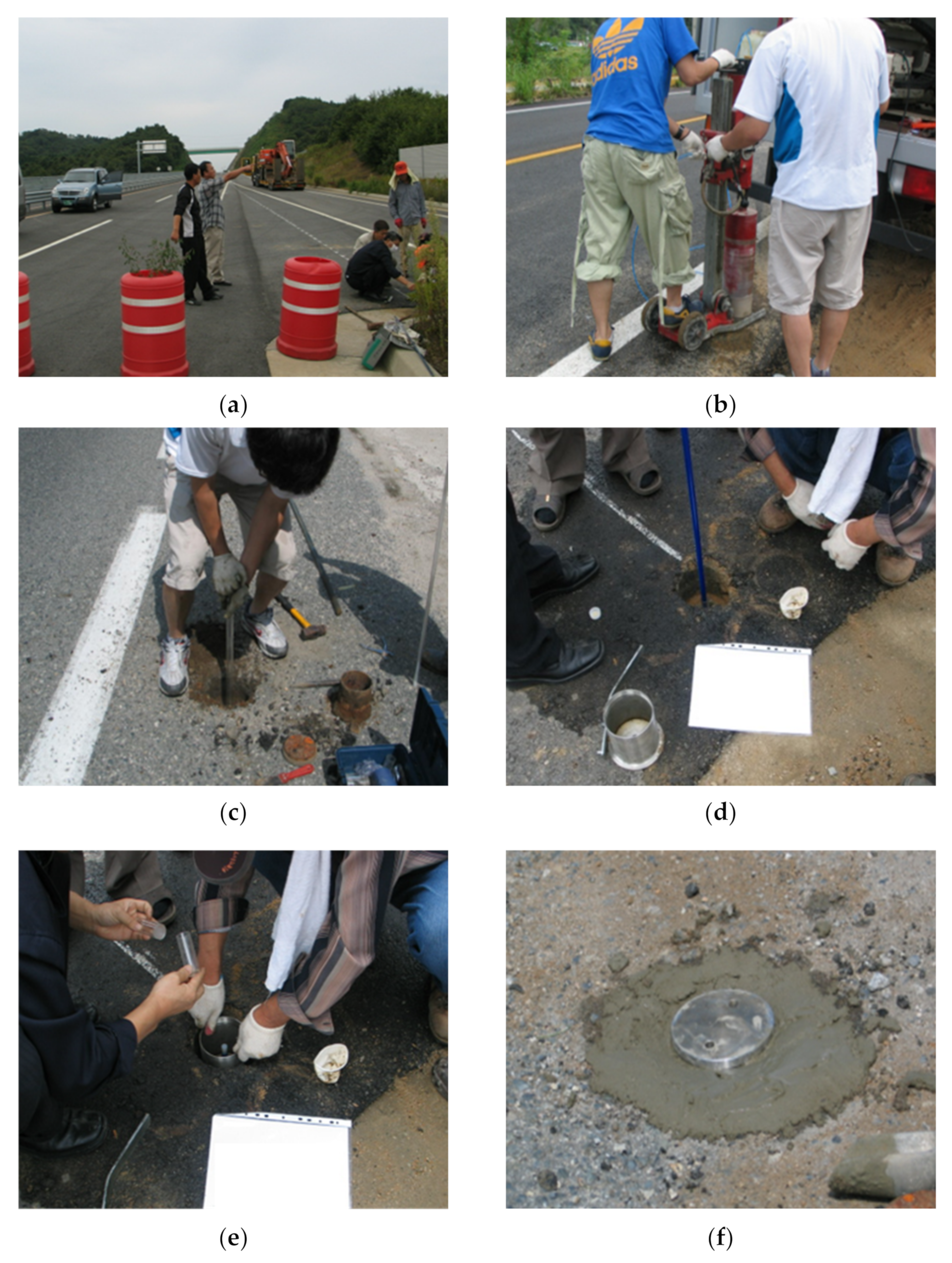
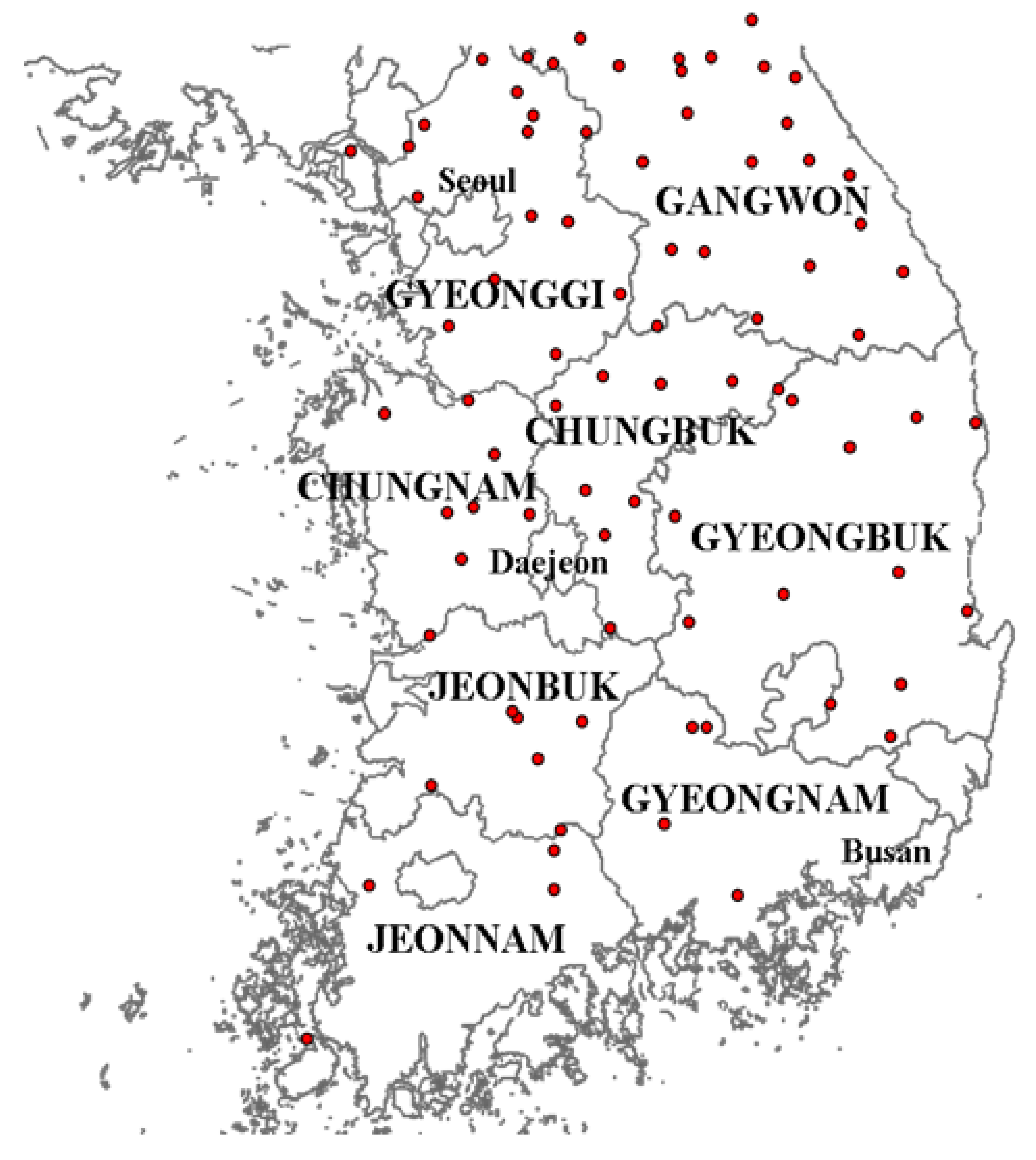
2.1. Field Experiment
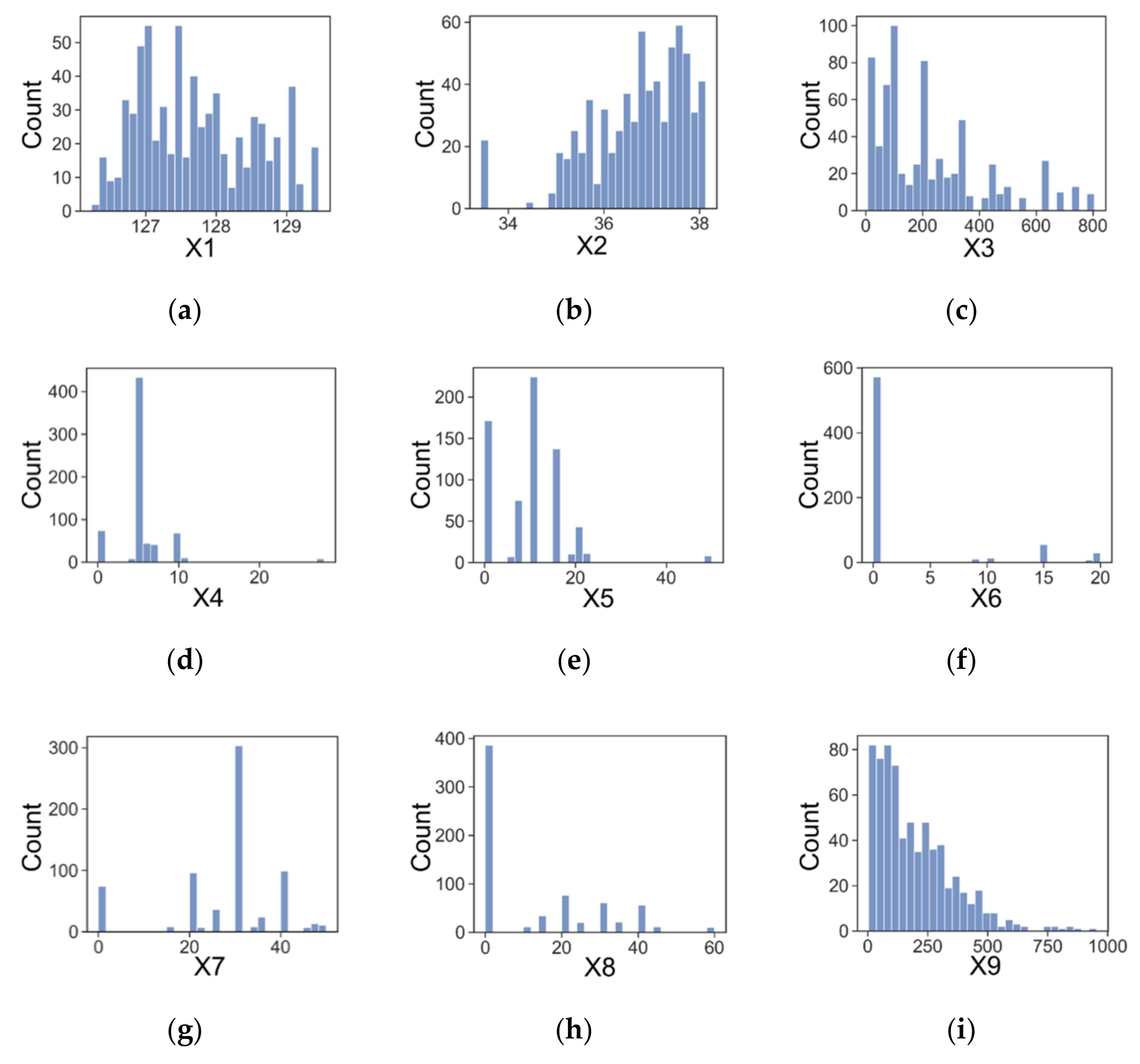
2.2. Data Analysis
3. Methodology
3.1. Machine Learning Techniques
3.2. Dataset Partition and Scaling
3.3. Performance Measurement and K-Fold Cross-Validation
3.4. Hyperparameter Tuning
4. Results and Discussion
4.1. Performance of Developed Models
4.2. Improved Performance after Hyperparameter Tunings
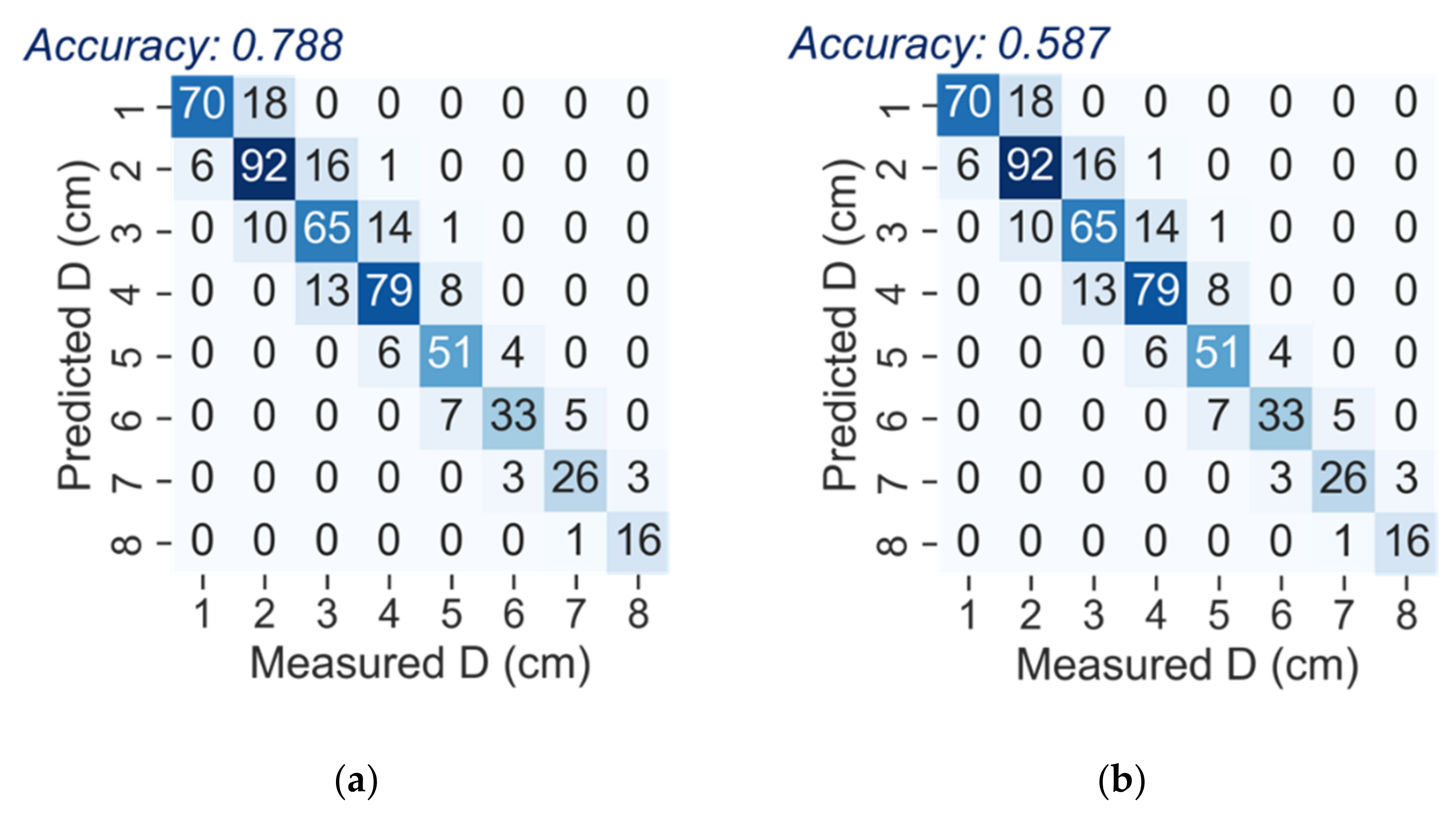
4.3. Prediction of Each Level of Frost Depth (Confusion Matrix)
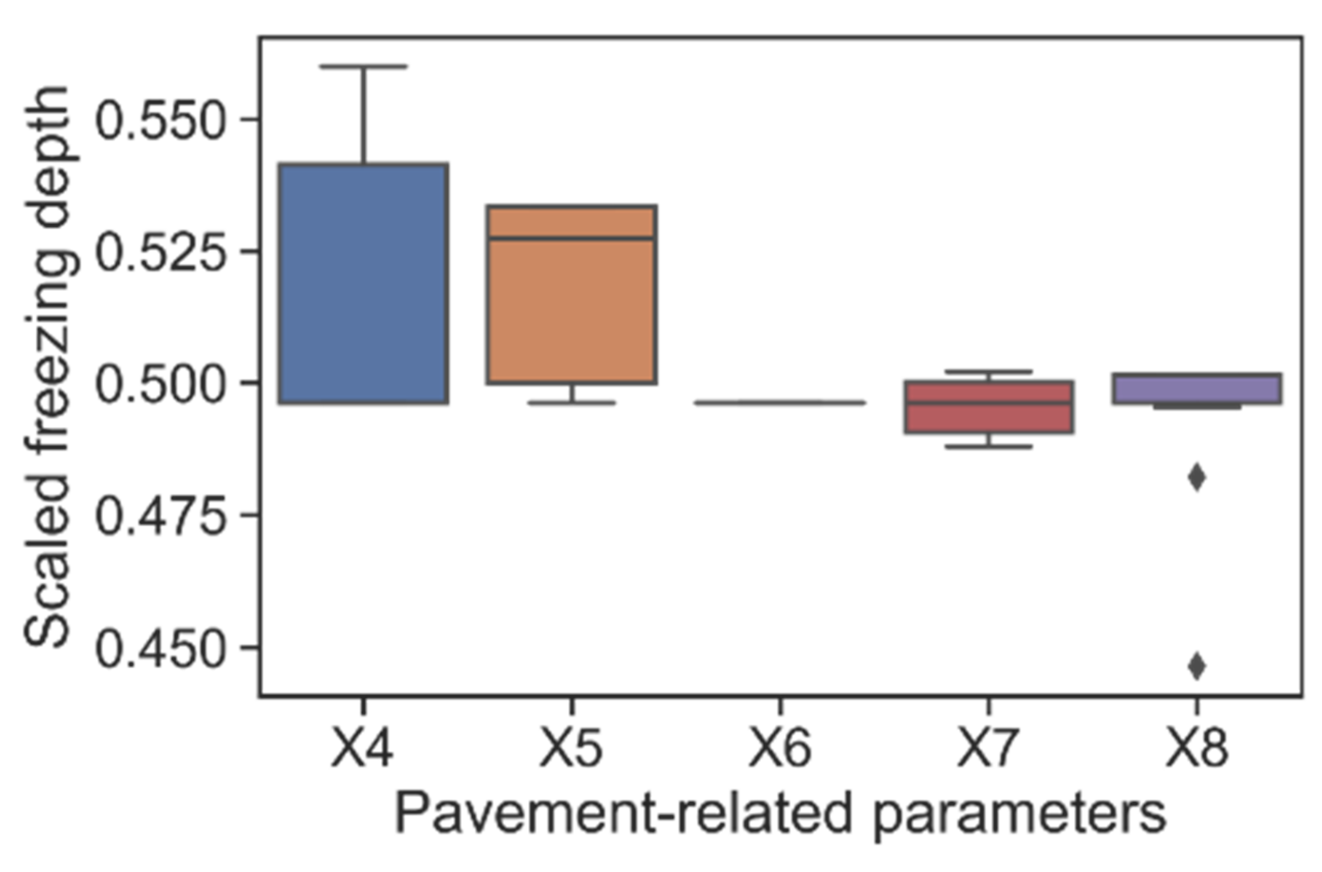
4.4. Sensitivity of Pavement-Related Predictors for Predicting Frost Depth
5. Conclusions
- (1)
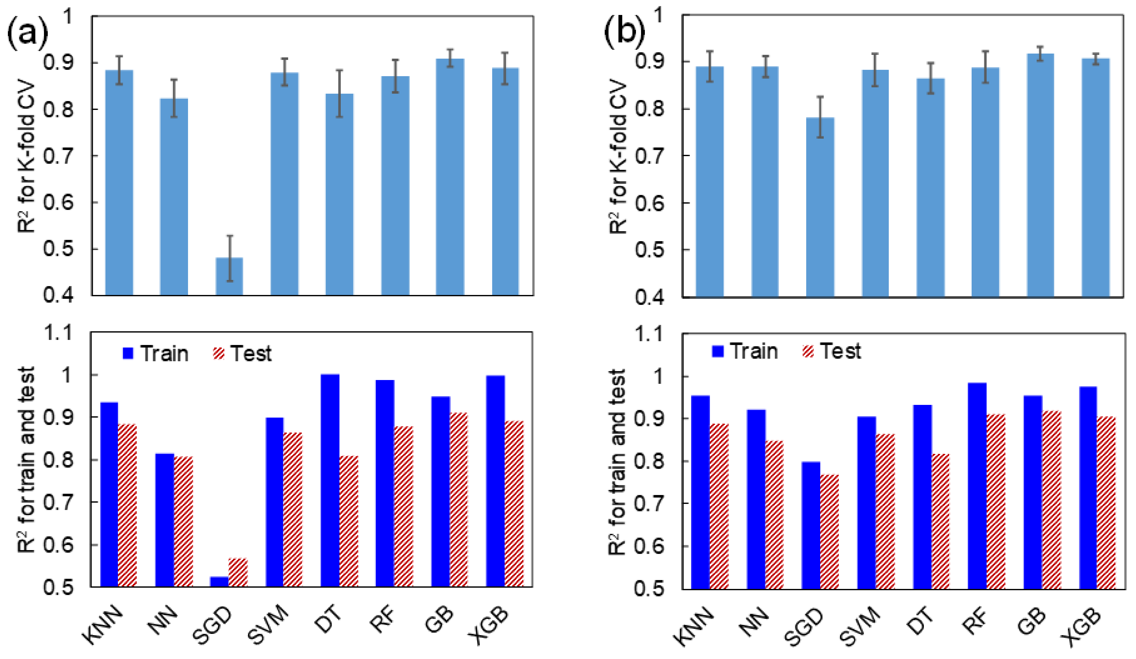
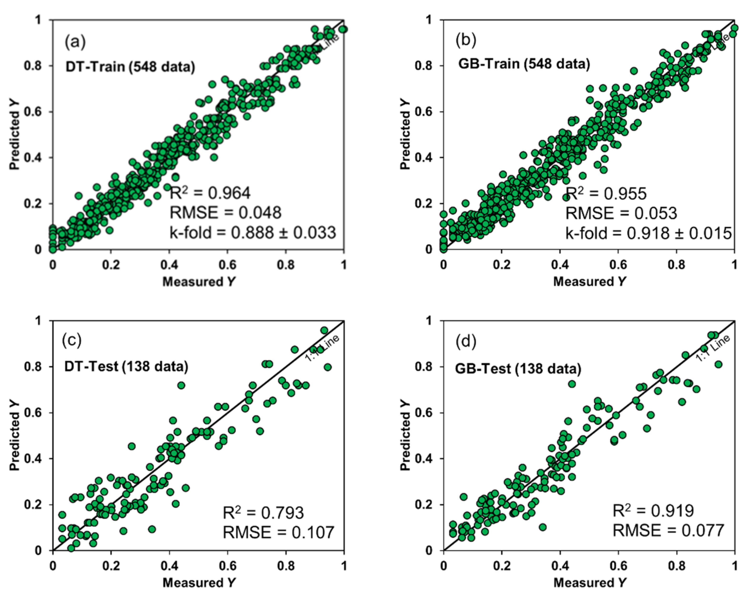
- The evaluated R2 and RMSE values indicated that ensemble ML algorithms (RF, GB, and XGB) showed higher performance than single ML algorithms (KNN, NN, SGD, SVM, and DT). After performing hyperparameter tuning, GB showed the best performance among the eight ML algorithms.
- (2)
- The performance was improved more significantly after hyperparameter tuning for five single ML models than for three ensemble ML models, which implies the ensemble ML algorithms can be used to develop models for predicting frost depth with reasonably high performance without performing hyperparameter tuning.
- (3)
- The developed best performing GB model can be used to assess the predictability of frost depth in a predefined number of categories using the confusion matrix. However, the low prediction accuracy in the confusion matrix for eight categories implies that a more accurate model would be required to achieve high predictability of frost depth.
- (4)
- The result of sensitivity analysis for pavement-related predictors implies that the thickness of the asphalt surface is the most critical factor affecting the frost depth of soils.
Author Contributions
Funding
Institutional Review Board Statement
Informed Consent Statement
Data Availability Statement
Conflicts of Interest
References
- Li, Q.; Wei, H.; Han, L.; Wang, F.; Zhang, Y.; Han, S. Feasibility of Using Modified Silty Clay and Extruded Polystyrene (XPS) Board as the Subgrade Thermal Insulation Layer in a Seasonally Frozen Region, Northeast China. Sustainability 2019, 11, 804. [Google Scholar] [CrossRef] [Green Version]
- Penner, E. The Mechanism of Frost Heaving in Soils. Highw. Res. Board Bull. 1959, 225, 1–22. [Google Scholar]
- Zhang, Y.; Korkiala-Tanttu, L.K.; Gustavsson, H.; Miksic, A. Assessment for Sustainable Use of Quarry Fines as Pavement Construction Materials: Part I-Description of Basic Quarry Fine Properties. Materials 2019, 12, 1209. [Google Scholar] [CrossRef] [PubMed] [Green Version]
- Vaitkus, A.; Gražulyte, J.; Skrodenis, E.; Kravcovas, I. Design of Frost Resistant Pavement Structure Based on Road Weather Stations (RWSs) Data. Sustainability 2016, 8, 1328. [Google Scholar] [CrossRef] [Green Version]
- Liu, Y.; Li, D.; Chen, L.; Ming, F. Study on the Mechanical Criterion of Ice Lens Formation Based on Pore Size Distribution. Appl. Sci. 2020, 10, 8981. [Google Scholar] [CrossRef]
- Yao, L.Y.; Broms, B.B. Excess Pore Pressures Which Develop during Thawing of Frozen Fine-Grained Subgrade Soils. Highw. Res. Rec. 1965, 39–57. [Google Scholar]
- Eigenbrod, K.D.; Knutsson, S.; Sheng, D. Pore-Water Pressures in Freezing and Thawing Fine-Grained Soils. J. Cold Reg. Eng. 1996, 10, 77–92. [Google Scholar] [CrossRef]
- Simonsen, E.; Isacsson, U. Thaw Weakening of Pavement Structures in Cold Regions. Cold Reg. Sci. Technol. 1999, 29, 135–151. [Google Scholar] [CrossRef]
- Remišová, E.; Decký, M.; Podolka, L.; Kováč, M.; Vondráčková, T.; Bartuška, L. Frost Index from Aspect of Design of Pavement Construction in Slovakia. Procedia Earth Planet. Sci. 2015, 15, 3–10. [Google Scholar] [CrossRef] [Green Version]
- Fu, J.; Shen, A. Meso- and Macro-Mechanical Analysis of the Frost-Heaving Effect of Void Water on Asphalt Pavement. Materials 2022, 15, 414. [Google Scholar] [CrossRef]
- Chisholm, R.A.; Phang, W.A. Measurement and Prediction of Frost Penetration in Highways. Transp. Res. Rec. 1983, 918, 1–10. [Google Scholar]
- Kahimba, F.C.; Ranjan, R.S.; Mann, D.D. Modeling Soil Temperature, Frost Depth, and Soil Moisture Redistribution in Seasonally Frozen Agricultural Soils. Appl. Eng. Agric. 2009, 25, 871–882. [Google Scholar] [CrossRef]
- Orakoglu, M.E.; Liu, J.; Tutumluer, E. Frost Depth Prediction for Seasonal Freezing Area in Eastern Turkey. Cold Reg. Sci. Technol. 2016, 124, 118–126. [Google Scholar] [CrossRef]
- Roustaei, M.; Hendry, M.T.; Roghani, A. Investigating the Mechanism of Frost Penetration under Railway Embankment and Projecting Frost Depth for Future Expected Climate: A Case Study. Cold Reg. Sci. Technol. 2022, 197, 103523. [Google Scholar] [CrossRef]
- Rajaei, P.; Baladi, G.Y. Frost Depth: General Prediction Model. Transp. Res. Rec. J. Transp. Res. Board 2015, 2510, 74–80. [Google Scholar] [CrossRef]
- Iwata, Y.; Hirota, T.; Suzuki, T.; Kuwao, K. Comparison of Soil Frost and Thaw Depths Measured Using Frost Tubes and Other Methods. Cold Reg. Sci. Technol. 2012, 71, 111–117. [Google Scholar] [CrossRef]
- Kim, H.S.; Lee, J.; Kim, Y.S.; Kang, J.-M.; Hong, S.-S. Experimental and Field Investigations for the Accuracy of the Frost Depth Indicator with Methylene Blue Solution. J. Korean Geosynth. Soc. 2013, 12, 75–79. [Google Scholar] [CrossRef]
- Gandahi, R. Determination of the Ground Frost Line by Means of a Simple Type of Frost Depth Indicator; Statens Väginstitut: Stockholm, Sweden, 1963; pp. 14–19. [Google Scholar]
- Hong, S.; Kim, Y.; Kim, S. A Study on the Frost Penetration Depth in Pavements; Korea Institute of Civil Engineering and Building Technology: Goyang, Korea, 2019; pp. 57–59. [Google Scholar]
- Liakos, K.; Busato, P.; Moshou, D.; Pearson, S.; Bochtis, D. Machine Learning in Agriculture: A Review. Sensors 2018, 18, 2674. [Google Scholar] [CrossRef] [Green Version]
- Garg, R.; Aggarwal, H.; Centobelli, P.; Cerchione, R. Extracting Knowledge from Big Data for Sustainability: A Comparison of Machine Learning Techniques. Sustainability 2019, 11, 6669. [Google Scholar] [CrossRef] [Green Version]
- Nguyen, H.; Vu, T.; Vo, T.P.; Thai, H.-T. Efficient Machine Learning Models for Prediction of Concrete Strengths. Constr. Build. Mater. 2021, 266, 120950. [Google Scholar] [CrossRef]
- Guo, G.; Wang, H.; Bell, D.; Bi, Y.; Greer, K. KNN Model-Based Approach in Classification. In On The Move to Meaningful Internet Systems 2003: CoopIS, DOA, and ODBASE—OTM 2003; Springer: Berlin/Heidelberg, Germany, 2003; pp. 986–996. [Google Scholar]
- Abiodun, O.I.; Jantan, A.; Omolara, A.E.; Dada, K.V.; Mohamed, N.A.; Arshad, H. State-of-the-Art in Artificial Neural Network Applications: A Survey. Heliyon 2018, 4, e00938. [Google Scholar] [CrossRef] [PubMed] [Green Version]
- Géron, A. Hands-On Machine Learning with Scikit-Learn, Keras, and TensorFlow: Concepts, Tools, and Techniques to Build Intelligent Systems; O’Reilly Media: Newton, MA, USA, 2019; ISBN 1492032611. [Google Scholar]
- Cortes, C.; Vapnik, V. Support-Vector Networks. Mach. Learn. 1995, 20, 273–297. [Google Scholar] [CrossRef]
- Myles, A.J.; Feudale, R.N.; Liu, Y.; Woody, N.A.; Brown, S.D. An Introduction to Decision Tree Modeling. J. Chemom. 2004, 18, 275–285. [Google Scholar] [CrossRef]
- Belgiu, M.; Drăguţ, L. Random Forest in Remote Sensing: A Review of Applications and Future Directions. ISPRS J. Photogramm. Remote Sens. 2016, 114, 24–31. [Google Scholar] [CrossRef]
- Natekin, A.; Knoll, A. Gradient Boosting Machines, a Tutorial. Front. Neurorobot. 2013, 7. [Google Scholar] [CrossRef] [Green Version]
- Chen, T.; Guestrin, C. XGBoost: A Scalable Tree Boosting System. In Proceedings of the 22nd ACM SIGKDD International Conference on Knowledge Discovery and Data Mining, San Francisco, CA, USA, 13–17 August 2016; ACM: New York, NY, USA, 2016; pp. 785–794. [Google Scholar]


| Predictors | Mean ± Std. | Min | Q1 | Median | Q3 | Max | CV |
|---|---|---|---|---|---|---|---|
| X1 | 127.72 ± 0.80 | 126.23 | 127.02 | 127.60 | 128.37 | 129.46 | 0.01 |
| X2 | 36.70 ± 1.04 | 33.43 | 36.07 | 36.86 | 37.51 | 38.13 | 0.03 |
| X3 | 225.63 ± 193.90 | 7.00 | 73.00 | 192.00 | 328.00 | 805.00 | 0.86 |
| X4 | 5.48 ± 3.46 | 0.00 | 5.00 | 5.00 | 5.00 | 28.00 | 0.63 |
| X5 | 9.59 ± 7.73 | 0.00 | 6.00 | 10.00 | 15.00 | 50.00 | 0.81 |
| X6 | 2.56 ± 5.93 | 0.00 | 0.00 | 0.00 | 0.00 | 20.00 | 2.31 |
| X7 | 27.32 ± 11.75 | 0.00 | 20.00 | 30.00 | 30.00 | 50.00 | 0.43 |
| X8 | 12.45 ± 15.92 | 0.00 | 0.00 | 0.00 | 25.00 | 60.00 | 1.28 |
| X9 | 195.50 ± 159.18 | 3.94 | 71.38 | 155.11 | 283.40 | 954.16 | 0.81 |
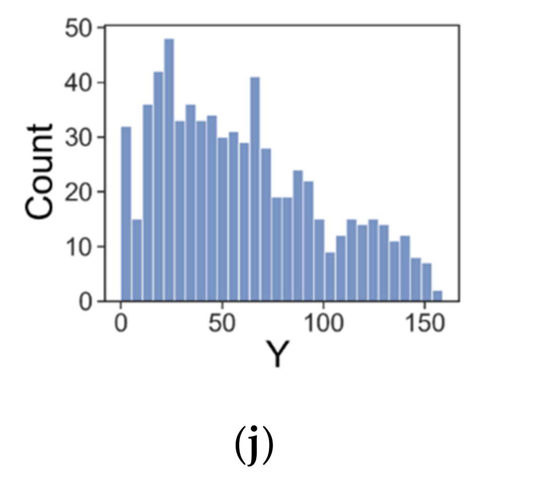
| Y | 59.75 ± 39.35 | 0.00 | 26.05 | 53.75 | 87.00 | 159.00 | 0.66 |
| ML Technique | Features | Reference |
|---|---|---|
| KNN | Non-parametric algorithm, high-speed training, computationally expensive | [23] |
| NN | Ability to learn nonlinear model, sensitive to scaling of predictors, need to optimize number of layers and neurons | [24] |
| SGD | Optimization of differentiable cost function, ability to train big dataset, hyperparameters tuning is necessary | [25] |
| SVM | Non-parametric algorithm, ability to model high-dimensional data, computationally expensive | [26] |
| DT | Non-parametric algorithm, ability to obtain predictor importance, high chance of overfitting issues | [27] |
| RF | Homogenous ensemble algorithm, ability to select base ML algorithm (e.g., DT, SVM, NN, KNN) | [28] |
| GB | Sequential learning method, minimize the loss function by parameterizing DT, | [29] |
| XGB | Addition of regularization term into GB to solve overfitting issues, many loss functions available | [30] |
| ML Technique | R2 | RMSE | ||||
|---|---|---|---|---|---|---|
| K-Fold | Train | Test | K-Fold | Train | Test | |
| KNN | 0.884 ± 0.031 | 0.935 | 0.884 | 0.082 ± 0.009 | 0.063 | 0.085 |
| NN | 0.823 ± 0.040 | 0.814 | 0.805 | 0.103 ± 0.011 | 0.107 | 0.108 |
| SGD | 0.480 ± 0.049 | 0.523 | 0.569 | 0.179 ± 0.016 | 0.175 | 0.146 |
| SVM | 0.880 ± 0.028 | 0.898 | 0.863 | 0.083 ± 0.007 | 0.078 | 0.094 |
| DT | 0.834 ± 0.051 | 1.000 | 0.808 | 0.098 ± 0.013 | 0.000 | 0.106 |
| RF | 0.872 ± 0.035 | 0.987 | 0.877 | 0.872 ± 0.035 | 0.029 | 0.079 |
| GB | 0.910 ± 0.019 | 0.950 | 0.910 | 0.073 ± 0.008 | 0.055 | 0.077 |
| XGB | 0.888 ± 0.033 | 0.999 | 0.892 | 0.081 ± 0.008 | 0.009 | 0.078 |
| ML Technique | R2 | RMSE | ||||
|---|---|---|---|---|---|---|
| K-Fold | Train | Test | K-Fold | Train | Test | |
| KNN | 0.889 ± 0.032 | 0.954 | 0.889 | 0.079 ± 0.009 | 0.053 | 0.081 |
| NN | 0.889 ± 0.022 | 0.920 | 0.847 | 0.081 ± 0.010 | 0.070 | 0.093 |
| SGD | 0.782 ± 0.043 | 0.798 | 0.769 | 0.111 ± 0.010 | 0.111 | 0.118 |
| SVM | 0.882 ± 0.030 | 0.905 | 0.865 | 0.082 ± 0.008 | 0.076 | 0.094 |
| DT | 0.865 ± 0.042 | 0.932 | 0.818 | 0.088 ± 0.011 | 0.065 | 0.103 |
| RF | 0.888 ± 0.033 | 0.985 | 0.910 | 0.079 ± 0.009 | 0.030 | 0.076 |
| GB | 0.918 ± 0.015 | 0.955 | 0.919 | 0.070 ± 0.007 | 0.053 | 0.068 |
| XGB | 0.906 ± 0.014 | 0.975 | 0.904 | 0.076 ± 0.005 | 0.040 | 0.075 |
| ML Technique | Range of Hyperparameters | Tuned Hyperparameters |
|---|---|---|
| KNN | leaf_size = 10, 15, 20, …, 40, 45, 50 n_neighbors = 3, 4, 5, …, 8, 9, 10 | 10 3 |
| NN | α = 0.00001, 0.0001, 0.001, 0.01, 0.1 early_stopping = True, False hidden_layer_sizes = [50], [100], [100, 100], [50, 50, 50] | 0.0001 True [50, 50, 50] |
| SGD | α = 0.0001, 0.0001, 0.001, 0.005 eta0 = 0.005, 0.01, 0.03, 0.05, 0.1, 0.2 max_iter = 500, 600, 700, …, 1800, 1900, 2000 | 0.0001 0.2 1200 |
| SVM | C = 0.5, 0.6, 0.7, …, 1.3, 1.4, 1.5 gamma = 0.5, 0.55, 0.6, …, 0.9, 0.95, 1.0 kernel = ’linear’, ’poly’, ’rbf’, ‘sigmoid’ | 1.4 1.9 ’rbf’ |
| DT | min_samples_leaf = 1, 2, 3, …, 8, 9, 10 min_samples_split = 1, 2, 3, …, 8, 9, 10 | 7 3 |
| RF 1 | n_estimators = 50, 60, 70, …, 280, 290, 300 | 280 |
| GB 1 | max_depth = 2, 3, 4, …, 8, 9, 10 n_estimators = 20, 30, 40, …, 280, 290, 300 | 2 270 |
| XGB 1 | max_depth = 2, 3, 4, …, 8, 9, 10 n_estimators = 20, 30, 40, …, 280, 290, 300 | 4 50 |
Publisher’s Note: MDPI stays neutral with regard to jurisdictional claims in published maps and institutional affiliations. |
© 2022 by the authors. Licensee MDPI, Basel, Switzerland. This article is an open access article distributed under the terms and conditions of the Creative Commons Attribution (CC BY) license (https://creativecommons.org/licenses/by/4.0/).
Share and Cite
Choi, H.-J.; Kim, S.; Kim, Y.; Won, J. Predicting Frost Depth of Soils in South Korea Using Machine Learning Techniques. Sustainability 2022, 14, 9767. https://doi.org/10.3390/su14159767
Choi H-J, Kim S, Kim Y, Won J. Predicting Frost Depth of Soils in South Korea Using Machine Learning Techniques. Sustainability. 2022; 14(15):9767. https://doi.org/10.3390/su14159767
Chicago/Turabian StyleChoi, Hyun-Jun, Sewon Kim, YoungSeok Kim, and Jongmuk Won. 2022. "Predicting Frost Depth of Soils in South Korea Using Machine Learning Techniques" Sustainability 14, no. 15: 9767. https://doi.org/10.3390/su14159767
APA StyleChoi, H.-J., Kim, S., Kim, Y., & Won, J. (2022). Predicting Frost Depth of Soils in South Korea Using Machine Learning Techniques. Sustainability, 14(15), 9767. https://doi.org/10.3390/su14159767