The Relationship between Economic Growth and Disaster Losses-Based on Linear and Nonlinear ARDL Model in China

Abstract

China is a country with one of the most disaster losses in the world. In this paper, a comprehensive evaluation of disaster losses in China was carried out based on the TOPSIS model of entropy weight. Then, linear and nonlinear models were established, and the relationship between economic growth and disaster losses was analyzed using the ARDL model, which included energy consumption and fixed asset investments. The results showed a significant inverted U-shaped relationship between disaster losses and economic growth; that is, smaller disaster losses helped increase economic growth, but larger disaster losses inhibited economic growth. In the long run, the increase in fossil energy consumption and new energy consumption promoted economic growth, but the role of fossil energy was more significant than that of new energy. We also found that fixed asset investment had a negative effect on economic growth.

1. Introduction

In recent years, the frequency of natural disasters has been increasing worldwide, and the resulting losses have been expanding. Before the 1990s, the economic impact of natural disasters did not receive enough attention from researchers. In the 20th century, after the mid-1990s, a series of natural disasters occurred, all of which brought considerable damage and had a huge impact on society. At the same time, due to the increasingly complicated nature of the social economy and the related forms among various departments and industries being more diversified, the methods and processes of the spread of disasters economically impact the socialized production system, industrial chain, and inter-regional economic connection are further complicated. Historical statistics show that the frequency and scale of natural disasters are increasing day by day. Therefore, understanding the social and economic impact of natural disasters has become a matter of global importance.

China is a country with a high frequency of regional natural disasters. Floods, droughts, typhoons, earthquakes, mudslides, and other kinds of natural disasters pose serious threats to people’s lives and property safety and also affect social stability and economic development. According to data from China Statistical Yearbook, natural disasters affected more than 2 million people annually in China from 2010 to 2018, as shown in Figure 1.

In addition, the direct economic losses caused by natural disasters in recent years exceeded 5% of the GDP on average (Figure 2).

This paper studied the relationship between Chinese natural disaster losses and economic growth to discuss the linear or nonlinear relationship between them, and figure out the impact mechanism of natural disasters on the economy. Section 2 provides a review of the literature, and in Section 3, the TOPSIS model of entropy weight is used to comprehensively measure the disaster losses in China. In Section 4, the ARDL model is adopted to reveal the relationship between natural disaster losses and economic growth in China. The final section provides a summary and proposes some suggestions.

2. Literature Review

One widely accepted view is that natural disasters have a negative impact on economic growth, and the damage is significant. For example, Srobl examined the macroeconomic impact of natural disasters on developing countries through the investigation of hurricane attacks in Central America and the Caribbean and showed that, on average, the hurricane hit decreased output by at least 0.83% [1]. Cho estimated the impact of Typhoon Rusa on South Korea’s Gross Domestic Product (GDP) as a decrease of 1.18% [2]. Sometimes disasters even affect the economy for a long time. Coffman et al. found that the economic damage caused by Hurricane Iniki in 1992 lasted 7 to 8 years, Kauai, Hawaii before the economy recovered to its pre-hurricane level [3].

Disasters can have multiple effects that would hamper economic growth. Beson found that countries more frequently affected by natural disasters had relatively low economic growth rates [4]. One of the reasons is that disasters cause huge losses, and the increased demand for disaster relief materials squeezes resources for economic development and thus curbs economic growth [5]. Disasters in a region have an impact on economic losses, including damage to infrastructure in the area where the disaster occurs, and also influences the level of income distribution and poverty [6,7]. Furthermore, the impact of disasters on economic growth may vary depending on the level of development. Raddatz concluded that the economic growth of low-income countries is more vulnerable to climate disasters by studying disaster data from 112 countries [8]. Noy believed that natural disasters negatively affect the economy in the short term, but there were differences in different regions. Developed countries were more resilient to the impact of disasters, while developing countries were more vulnerable to the consequences of natural disasters [9]. Yan and Li found that low levels of disaster losses can promote economic growth, but the promotion effect decreases as disaster losses increase, and sustained disaster losses will have a significant negative impact on the economy [10].

Other studies express opposite views on the relationship between disasters and economic growth, instead believing that disasters can also promote economic growth to a certain extent. Albala et al., through a case study of related disasters in developing countries, found that the economy of most countries grew rapidly after disasters, indicating that natural disasters can promote economic development to a certain extent [11]. Skidemore et al. studied the impact of meteorological disasters and geological disasters on economic growth and found that geological disasters had a negative impact on economic growth, while meteorological disasters had a positive, promotional effect on economic growth [12]. Davis and Raschky also found that natural disasters can promote economic growth to a certain extent [13,14]. Related studies have found that there is no necessary link between disasters and economic losses, such as Cavallo et al., who showed that there was no significant interaction between natural disasters and economic growth [15].

3. Disaster Losses Measurement Based on Entropy Weight TOPSIS Model

The TOPSIS comprehensive evaluation method, known as an approximate ideal ranking method, is a decision-making method in systems science [16]. Its main purpose is to take the distance as an evaluation standard and measure the comprehensive level as the degree of closeness. Entropy is a measure of the disorder of a system. When the system can exist in more than one state, the probability of each state is $p_i(i=1,2,\dots ,m)$, then the entropy of the system is defined as:

$$E=-{\displaystyle \sum _{i=1}^m{p}_i}\ln p_i$$

The steps of the TOPSIS evaluation model based on entropy weight are as follows:

Step 1: Construction of the initial decision matrix. The initial decision matrix is constructed as follows:

$$R=\left(\begin{array}{cccc}{r}_{11}& r_{12}& \dots & r_{1n}\\ r_{21}& r_{22}& \dots & r_{2n}\\ \dots & \dots & \dots & \dots \\ r_{m1}& r_{m2}& \dots & r_{mn}\end{array}\right)$$

where R is the initial decision matrix, m is the number of nodes for suitability evaluation, n is the number of factors, r_ij is the analyzed values of each sampled parameter, i = 0, 1, 2, …, m, and j = 0, 1, 2, …, n.

Step 2: Normalization of the initial decision matrix. It is necessary to normalize the matrix since the dimension and metric of the data are not uniform. The normalized decision matrix can be expressed as follows:

$$V=\left(\begin{array}{cccc}{v}_{11}& v_{12}& \dots & v_{1n}\\ v_{21}& v_{22}& \dots & v_{2n}\\ \dots & \dots & \dots & \dots \\ v_{m1}& v_{m2}& \dots & v_{mn}\end{array}\right)$$

where V is the normalized decision matrix, and

$$v_{ij}=\frac{r_{ij}-\min r_{.j}}{\max r_{.j}-\min r_{.j}}, \cos \mathrm{t} \mathrm{type}.$$

$$v_{ij}=\frac{\max r_{.j}-r_{ij}}{\max r_{.j}-\min r_{.j}}, \mathrm{efficiency} \mathrm{type}.$$

Step 3: Calculation of the entropy. The entropy of each factor can is calculated as follows:

$$e_j=-k{\displaystyle \sum _{i=1}^m{y}_{ij}\ln y_{ij}},y_{ij}=\frac{v_{ij}+1}{{\displaystyle \sum _{i=1}^m(v_{ij}+1)}}$$

where e_j is the entropy of each factor and $k=1/\ln m$.

Step 4: Calculation of the weight. The weight of each factor can is calculated as follows:

$$w_j=\frac{(1-e_j)}{n-{\displaystyle \sum _{j=1}^n{e}_j}},$$

where $w_j\in [0,1],{\displaystyle \sum _{j=1}^n{w}_j}=1$, are the weights of each factor.

Step 5: Construction of the weighted decision matrix. The weight calculated above is assigned to the normalized decision matrix as

$$Y=\left(\begin{array}{cccc}{y}_{11}& y_{12}& \cdots & y_{1n}\\ y_{21}& y_{22}& \cdots & y_{2n}\\ ⋮& ⋮& ⋮& ⋮\\ y_{n1}& y_{n2}& \cdots & y_{n3}\end{array}\right)=\left(\begin{array}{cccc}{v}_{11}{w}_1& v_{12}{w}_1& \dots & v_{1n}{w}_1\\ v_{21}{w}_2& v_{22}{w}_2& \dots & v_{2n}{w}_2\\ \dots & \dots & \dots & \dots \\ v_{m1}{w}_n& v_{m2}{w}_n& \dots & v_{mn}{w}_n\end{array}\right).$$

where Y is the weighted decision matrix.

Step 6: Determination of the positive and negative ideal reference points. The positive and negative ideal reference points can be outlined as follows:

$$Y^{+}=\{\underset{1\le i\le m}{\max }{y}_{ij}|i=1,2,‥,m\}=\{y_1^{+},y_2^{+}\dots y_m^{+}\},$$

$$Y^{-}=\{\underset{1\le i\le m}{\min }{y}_{ij}|i=1,2,‥,m\}=\{y_1^{-},y_2^{-}\dots y_m^{-}\}.$$

Step 7: Calculation of the distances to the positive and negative ideal reference points:

$$d_j^{+}=\sqrt{{\displaystyle \sum _{i=1}^m(y_i^{+}-y_{ij})}},d_j^{-}=\sqrt{{\displaystyle \sum _{i=1}^m(y_i^{-}-y_{ij})}}$$

Step 8: Calculation of the closeness coefficient, which can be calculated as

$$t_j=\frac{d_j^{-}}{d_j^{+}+d_j^{-}},$$

where t_i is the closeness coefficient.

In combination with the consequences caused by natural disasters, the affected population, dead population, emergency displaced population, direct economic losses, and affected area were selected as evaluation indicators.

Table 1. Statistical description of disaster variables.

Variables	Direct Economic Losses	Affected Area	Affected Population	Dead Population	Emergency Displaced Population
Mean	3220.61	39,365.42	33,610.22	6448.08	1005.56
Median	2586.35	40,540.00	36,287.45	2400.00	810.00
Maximum	11,752.40	54,690.00	49,745.90	88,928.00	2682.20
Minimum	1602.30	18,480.00	3977.90	589.00	211.10
Std. Dev.	2154.69	11,853.52	12,691.39	17,668.99	597.61

Source: Chinese Civil Affairs Statistical Yearbook.

shows the statistical description of the data.

The TOPSIS comprehensive evaluation model based on entropy weight was used for the comprehensive evaluation of disaster losses, and the results are shown in Figure 3.

4. Analysis of the Relationship between Carbon Emissions and Disaster Losses

4.1. Variables and ARDL Model

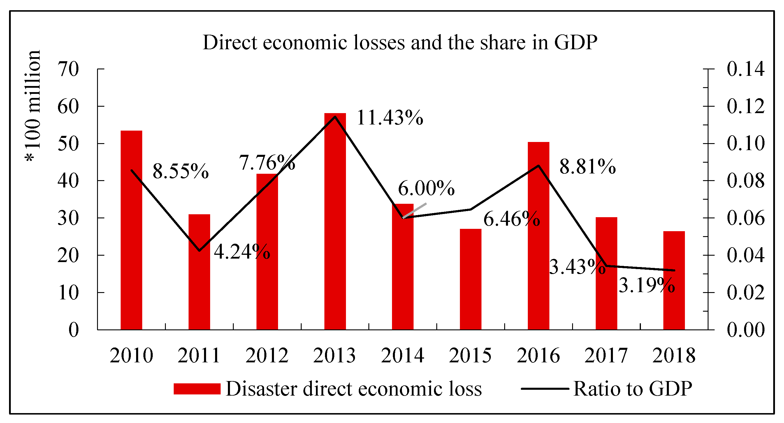
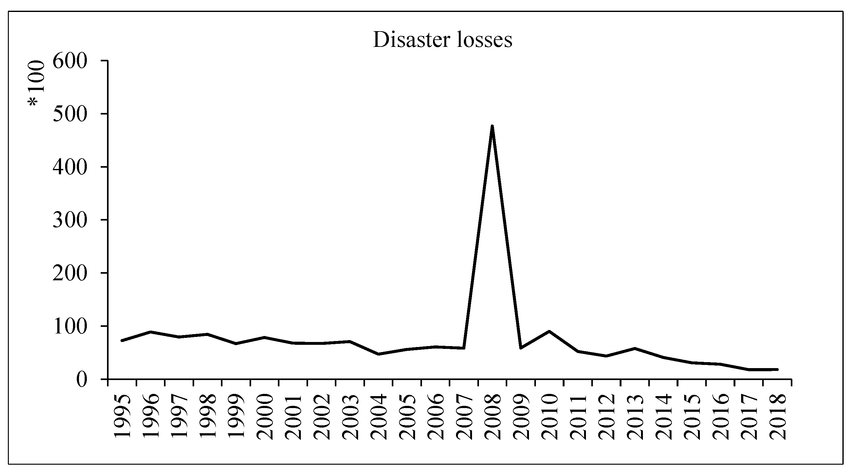
The role of new energy and fossil energy consumption on economic growth has been widely confirmed [17,18]. In this paper, the variables that affect economic growth were selected as fixed asset investment, fossil energy consumption, new energy consumption, and natural disaster losses. Among these, disaster losses are the calculation results presented in the above section. Other data are from the China Statistical Yearbook. The research interval is from 1995 to 2018.

Table 2. Variables and instructions.

Variables	Instructions
gdp	The real output, deflated by the 1990 level
fai	Investment in fixed assets, deflated by the 1990 level
een	Fossil energy consumption
nen	New energy consumption
disa	Disaster losses

Source: China Statistical Yearbook.

gives the variables and instructions.

Denote that ln(x) is the natural logarithm of variable x and ln(x)I represent the increment of ln(x). The statistical description of each variable is shown in

Table 3. Statistical description.

Variables	ln(gdp)	ln(fai)	ln(een)	ln(nen)	ln(disa)
Mean	10.859	10.861	12.369	9.999	8.579
Median	10.892	10.900	12.529	10.010	8.485
Maximum	11.815	12.322	12.889	11.125	10.926
Minimum	9.825	9.279	11.721	8.987	7.672

Source: Chinese Civil Affairs Statistical Yearbook.

.

Next, we used the autoregressive distributive lag model (ARDL) to estimate the relationship between carbon emissions and natural disaster losses. The ARDL model is very effective, even for different levels of integration and small sample sizes [19,20,21]. On the other hand, the ARDL bound testing technique even takes into account the endogenous regressors and only requires that the integral order of the regression variable not exceed 1.

Firstly, the following model was established to test whether there was a long-term cointegration relationship between variables:

$$\begin{array}{l}\mathrm{\Delta }\ln (gdp)I={\alpha }_1+{\displaystyle \sum _{i=1}^{k_1}{\beta }_{1i}}\mathrm{\Delta }\ln (gdp)I_{t-i}+{\displaystyle \sum _{i=1}^{k_2}{\beta }_{2i}}\mathrm{\Delta }\ln (een)I_{t-i}+{\displaystyle \sum _{i=1}^{k_3}{\beta }_{2i}}\mathrm{\Delta }\ln (nen)I_{t-i}\\ +{\displaystyle \sum _{i=1}^{k_4}{\beta }_{3i}}\mathrm{\Delta }\ln {(faiI)}_{t-i}+{\displaystyle \sum _{i=1}^{k_5}{\beta }_{4i}}\mathrm{\Delta }\ln {(disa)}_{t-i}+{\gamma }_1\ln (gdp)I_{t-1}+{\gamma }_2\ln (een)I_{t-1}\\ +{\gamma }_3\ln (een)I_{t-1}+{\gamma }_4\ln (fai)I_{t-1}+{\gamma }_5\ln {(disa)}_{t-1}+{\epsilon }_{1t}\hspace{1em}\hspace{1em}\end{array}$$

(1)

where ${\alpha }_1$ indicates the constant intercept,$\mathrm{\Delta }$ indicates the difference operator,${\gamma }_i$ indicates the short-run and long-run coefficients, respectively, and k_i is the optimal lag period that is determined by AIC or SC criterion.

The null hypothesis of no cointegration among the variables in the above Equation (1) was set as

$$H_0:{\gamma }_1={\gamma }_2={\gamma }_3={\gamma }_4={\gamma }_5=0$$

and the alternative hypothesis was set as

$$H_1:{\gamma }_1\ne 0\hspace{0.17em}or\hspace{0.17em}{\gamma }_2\ne 0\hspace{0.17em}or\hspace{0.17em}{\gamma }_3\ne 0or\hspace{0.17em}{\gamma }_4\ne 0or\hspace{0.17em}{\gamma }_5\ne 0\hspace{0.17em}.$$

If the value of the F-statistic was above the upper bound I(1), then we would reject the null hypothesis of no cointegration and conclude that there was a long-term stable relationship among the variables of interest; then, the short-run dynamics would be examined by the following error correction model (ECM).

$$\begin{array}{l}\mathrm{\Delta }\ln (gdp)I={\alpha }_3+{\displaystyle \sum _{i=1}^{{\xi }_1}{\rho }_{1i}}\mathrm{\Delta }\ln (gdp)I_{t-i}+{\displaystyle \sum _{i=1}^{{\xi }_2}{\rho }_{2i}}\mathrm{\Delta }\ln (een)I_{t-i}+{\displaystyle \sum _{i=1}^{{\xi }_3}{\rho }_{3i}}\mathrm{\Delta }\ln (nen)I_{t-i}\\ \hspace{1em}\hspace{1em}\hspace{1em}+{\displaystyle \sum _{i=1}^{{\xi }_4}{\rho }_{4i}}\mathrm{\Delta }\ln (fai)I_{t-i}+{\displaystyle \sum _{i=1}^{{\xi }_5}{\rho }_{5i}}\mathrm{\Delta }\ln {(disa)}_{t-i}+\lambda EC{M}_{t-1}+{\epsilon }_{2t}\end{array}$$

(2)

where ${\rho }_{ki}(k=1,2,3,4,5)$ are the short-run growth coefficients and $\lambda$ is the coefficient of error correction term, which shows the speed of adjustment towards long-run equilibrium.

Further, the following model can be established to estimate the long-term coefficients:

$$\begin{array}{l}\ln (gdp)I={\alpha }_2+{\displaystyle \sum _{i=1}^{{\delta }_1}{\eta }_{1i}}\ln (gdp)I_{t-i}+{\displaystyle \sum _{i=1}^{{\delta }_2}{\eta }_{2i}}\ln (een)I_{t-i}+{\displaystyle \sum _{i=1}^{{\delta }_2}{\eta }_{2i}}\ln (nen)I_{t-i}\\ \hspace{1em}\hspace{1em}\hspace{0.17em}\hspace{1em}+{\displaystyle \sum _{i=1}^{{\delta }_3}{\eta }_{3i}}\ln (fai)I_{t-i}+{\displaystyle \sum _{i=1}^{{\delta }_4}{\eta }_{4i}}\ln {(disa)}_{t-i}+{\epsilon }_{3t}\end{array}$$

(3)

where ${\eta }_{ki}(k=1,2,3,4)$ are the long-run growth coefficients.

4.2. Results Analysis

First of all, unit root tests were conducted, and the results are shown in

Table 4. Unit root tests.

Variables	Test Type	5% Level	T-Statistic	Prob.
ln(gdp)I	level	−3.632896	−1.540196	0.7834
	1st difference	−3.658446	−4.331060	0.0139 *
ln(een)I	level	−3.004861	−1.533965	0.4982
	1st difference	−3.012363	−3.991766	0.0064 *
ln(fai)I	level	−3.644963	−3.25911	0.9837
	1st difference	−3.658446	−4.542753	0.0092 *
ln(disa)	level	−3.622033	−4.619307	0.0065 *
ln(disa) * ln(disa)	level	−3.622033	−4.672785	0.0058 *

* indicates significance at a 5% probability level.

.

We found that variables were integrated with order zero I(0) or I(1), which indicated that the preconditions of the boundary cointegration test were satisfied. The optimal lag order was selected as 2 according to the AIC criterion, and the ARDL bounds test results are shown in

Table 5. Boundary co-integration test results of model 1.

Significance	10%		5%		1%
	I(0)	I(1)	I(0)	I(1)	I(0)	I(1)
Critical Value Bounds	2.20	3.09	2.56	3.49	3.29	4.37
F-Statistic	F = 7.302214

.

The results in Table 5 reveal that there exists a long-term equilibrium relationship among the various explanatory variables. The short-term estimation results based on ECM and the long-term estimation results of model 1 are shown in

Table 6. Short run coefficients.

Variables	Coefficient	Std. Error	T-Statistic	Prob.
d(ln(gdp)I(−1))	0.74999	0.099791	7.515585	0.0003
d(ln(disa))	−0.002986	0.001879	−1.58895	0.1632
d(ln(disa)(−1))	−0.009231	0.001558	−5.926444	0.0010
d(ln(fai)I)	−0.077158	0.017828	−4.328016	0.0049
d(ln(fai)I(−1))	−0.038881	0.015498	−2.508755	0.0460
d(ln(nen)I)	0.06142	0.010925	5.621976	0.0014
d(ln(nen)I(−1))	−0.044117	0.009014	−4.894484	0.0027
d(ln(een)I)	0.314848	0.03789	8.309447	0.0002
d(ln(een)I(−1))	−0.563146	0.054644	−10.30568	0.0000
CointEq(−1)	−0.826767	0.090241	−9.161735	0.0001
R2	0.957047

and

Table 7. The long-run coefficients.

Variables	Coefficient	Std. Error	T-Statistic	Prob.
ln(disa)	0.018152	0.004442	4.086328	0.0065
ln(fai)I	−0.055221	0.051423	−1.073862	0.3242
ln(een)I	0.442601	0.092770	4.770975	0.0031
ln(nen)I	0.039811	0.046665	0.853122	0.4263
C	−0.090547	0.035298	−2.565249	0.0426

, respectively.

In addition, the Ramsey RESET test in

Table 8. Diagnostic tests.

Diagnostic Test	Statistic	Prob.
LM test	0.3478	0.8404
Ramsey RESET test	3.8854	0.0037
Jarque–Bera test	2.9929	0.2239
ARCH test	0.0002	0.9913
Breusch–Godfrey	0.8102	0.6533
D.W. test	2.1662	/

also shows that there is a setting bias in the model.

Table 9. VIF tests.

Variable	Coefficient	Uncentered VIF	Centered VIF
ln(gdp)I(−1)	0.0332	260.4987	9.9242
ln(gdp)I(−2)	0.0515	416.0837	14.2891
ln(disa)	0.0009	22.3331	5.2048
ln(disa)(−1)	0.0007	17.5831	3.0690
ln(disa)(−2)	0.0007	15.9031	2.1514
ln(fai)I	0.0004	6.5566	2.4137
ln(fai)I(−1)	0.0004	6.0610	2.2690
ln(fai)I(−2)	0.0003	4.1302	1.6457
ln(nen)I	0.0042	21.3153	9.2274
ln(nen)I(−1)	0.0086	43.88395	19.8813
ln(nen)I(−2)	0.0079	40.20849	17.9757
ln(een)I	8.58 × 10−6	623.0242	3.5162
ln(een)I(−1)	1.66 × 10−5	1223.712	6.2682
ln(een)I(−2)	6.74 × 10−6	503.0009	2.3843
C	0.0016	1595.67	NA

shows the VIF test of the model. It can be seen that most of the Centered VIF value are less than 10, themulticollinearity on the whole can be almost negligibled.

Next, we turned to nonlinear analysis and expanded model 3 into the following form.

$$\begin{array}{l}\ln gdpI={\alpha }_4+{\displaystyle \sum _{i=1}^{{\delta }_1}{\eta }_{1i}}\ln (gdp)I_{t-i}+{\displaystyle \sum _{i=1}^{{\delta }_2}{\eta }_{2i}}\ln (een)I_{t-i}+{\displaystyle \sum _{i=1}^{{\delta }_3}{\eta }_{3i}}\ln (nen)I_{t-i}+{\displaystyle \sum _{i=1}^{{\delta }_4}{\eta }_{4i}}\ln (fai)I_{t-i}\\ \hspace{1em}\hspace{1em}\hspace{1em}\hspace{1em}+{\displaystyle \sum _{i=1}^{{\delta }_5}{\eta }_{5i}}\ln {(disa)}_{t-i}+\hspace{1em}{\displaystyle \sum _{i=1}^{{\delta }_6}{\eta }_{6i}}{(\ln (disa)\ast \ln (disa))}_{t-i}+{\epsilon }_{5t}\end{array}$$

(4)

Compared with the threshold regression model, the ARDL model, constructed as model 4, can analyze the short-term and long-term relationships between variables, although it cannot find multiple threshold values.

Table 10. The short-run coefficients.

Variables	Coefficient	Std. Error	T-Statistic	Prob.
d(ln(gdp)I(−1))	0.2631	0.0319	8.2608	0.0037
d(ln(disa))	0.1033	0.0075	13.6921	0.0008
d(ln(disa)(−1))	−0.0787	0.0067	−11.6927	0.0013
d(ln(disa) * ln(disa))	−0.0058	0.0004	−14.5870	0.0007
d(ln(disa) * ln(disa)(−1))	0.0041	0.0004	11.2809	0.0015
d(ln(fai)I)	−0.1568	0.0053	−29.3641	0.0001
d(ln(fai)I(−1))	−0.0777	0.0040	−19.2634	0.0003
d(ln(nen)I)	0.0878	0.0033	26.8876	0.0001
d(ln(nen)I(−1))	−0.0605	0.0025	−24.6893	0.0001
d(ln(een)I)	0.3306	0.0106	31.3328	0.0001
d(ln(een)I(−1))	−0.4612	0.0152	−30.3914	0.0001
CointEq(−1)	−0.4513	0.0131	−34.4072	0.0001
R2	0.998234

* indicates the multiplication.

and

Table 11. The long-run Coefficients.

Variables	Coefficient	Std. Error	T-Statistic	Prob.
lndisa	0.4303	0.1076	3.9988	0.0280
lndisa * lndisa	−0.0228	0.0060	−3.8157	0.0458
lnfaiI	−0.1332	0.0404	−3.2968	0.0458
lneenI	0.7019	0.1022	6.8677	0.0063
lnnenI	0.2413	0.0642	3.7604	0.0329
C	−1.9629	0.4888	−4.0160	0.0277

* indicates the multiplication.

show the estimation results for model 4.

Comparing the estimation results of the two models, it can be determined that the results of the nonlinear model are better than that of the linear model, and the quadratic function is more practical to describe the impact of disaster losses on economic growth.

From the perspective of fixed asset investment, both in the short run and the long run, it has a negative effect on economic growth that is, increasing the growth rate of fixed asset investment cannot effectively promote economic growth.

Whether in the long run or the short run, fossil energy consumption and new energy consumption have similar effects on economic growth, but the effect of fossil energy is more significant. Both types of energy consumption can drive economic growth in the long run, promote economic growth in the short run, but restrain economic growth in the first lag period.

From the results of the nonlinear model analysis, it can be seen that there is a significant inverted U-shaped relationship between economic growth and disaster loss; that is, a small degree of disaster contributes to economic growth, but a large degree of disaster loss will hinder economic growth.

Table 12. Diagnostic test of model 4.

Diagnostic Test	T-Statistic	Prob.
LM test	0.276768	0.7652
Ramsey RESET test	1.431627	0.1860
Jarque–Bera test	0.584567	0.7466
ARCH test	0.263787	0.6138
D.W. test		3.4852

shows that there is no sequence correlation or heteroscedasticity, and the residuals obey a normal distribution. The Ramsey test also shows that the model is reliable.

We have also built the Cointegration model (FMOLS) for comparison with the ARDL model, and the results are shown in

Table 13. The results of the FMOLS model.

Variable	Coefficient	Std. Error	T-Statistic	Prob.
dln(een)	0.22117	0.057324	3.858234	0.0014
dln(gt)	0.046992	0.038101	1.233361	0.2353
dln(nen)	0.002857	0.031252	0.091414	0.9283
lndisa	0.038866	0.057975	0.670394	0.5122
lndisa * lndisa	−0.001615	0.003123	−0.517206	0.6121
C	−0.143814	0.265624	−0.541419	0.5957

* indicates the multiplication.

.

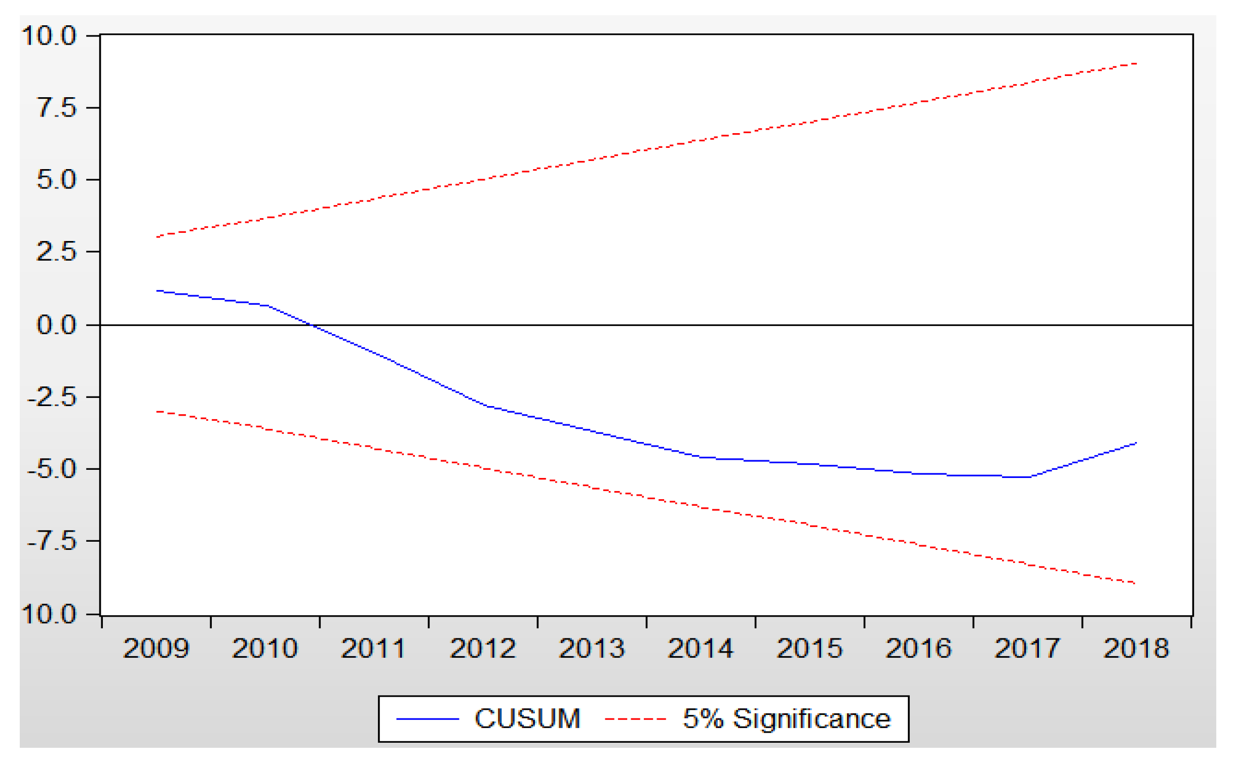
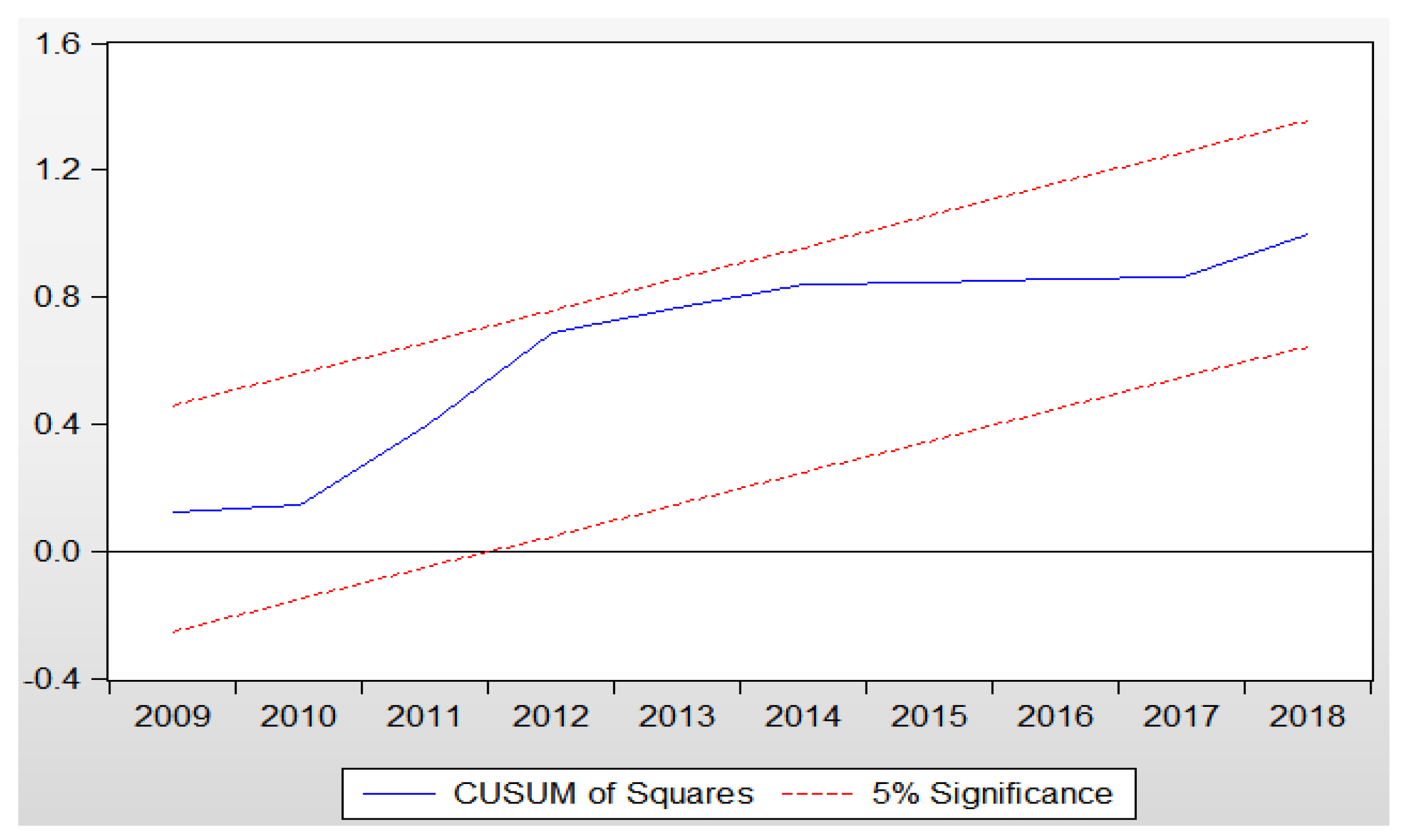
It can be determined that the fitting effect of the ARDL model is better than that of the FMOLS model. To avoid model unreliability caused by parameter instability, recursive residual accumulations (CUSUM) and recursive residual squares cumulative (CUSUMSQ) were used to test the theoretical model constructed above. The results are shown in Figure 4 and Figure 5, which show that the estimated coefficient of the nonlinear ARDL model has parameter stability.

5. Conclusions and Suggestions

In this paper, the entropy weight TOPSIS model was first used to measure the disaster losses in China, and then linear and nonlinear ARDL models were used to test the relationship between disaster losses and economic growth. The results showed a significant nonlinear relationship between the two. An inverted U-shaped relationship between disaster losses and economic growth tells us that when disaster losses reach a fixed threshold, it will restrain economic growth. Furthermore, we also found that faster fixed asset investment does not mean higher economic growth, and the role of fossil energy in promoting economic growth is now more pronounced than that of new energy.

According to the research results of this paper, in order to better promote economic growth, the following suggestions are provided. First of all, we should strengthen the construction of disaster prevention and mitigation infrastructure and enhance the ability of society to deal with disasters. Secondly, we should enhance the public’s awareness of disaster prevention and mitigation, enhance the public’s ability to save each other, and minimize disaster loss. Finally, in order to give full play to the role of new energy in energy conservation and emission reduction, it is necessary to provide a better market environment for the development of new energy, so that new energy forms a substituting role in the proportion and total amount, and better promotes economic development.

References

1. Strobl, E. The Economic Growth Impact of Natural Disasters in Developing Countries: Evidence from Hurricane Strikes in the Central American and Caribbean Regions. J. Dev. Econ. 2012, 97, 130–141. [Google Scholar] [CrossRef]
2. Cho, S. A Study on National economic impact by natural disaster-A case of typhoon. Product. Rev. 2010, 24, 273–290. [Google Scholar]
3. Coffman, M.; Noy, I. Hurricane Iniki: Measuring the Long-term Economic Impact of a Natural Disaster Using Synthetic Control. Environ. Dev. Econ. 2012, 17, 187–205. [Google Scholar] [CrossRef]
4. Benson, C. The Economy-Wide Impact of Natural Disasters in Developing Countries. Ph.D. Thesis, University of London, London, UK, 2003. [Google Scholar]
5. Kunreuther, H.; Pauly, M. Rules rather than discretion: Lessons from hurricane Katrina. J. Risk. Uncertain. 2006, 33, 101–116. [Google Scholar] [CrossRef] [Green Version]
6. Hidalgo, J.; Baez, A.A. Natural disasters. Crit. Care Clin. 2019, 35, 591–607. [Google Scholar] [CrossRef] [PubMed]
7. Groeschl, J. Poverty, inequality, and disasters—An introduction to the special issue. Econ. Disaster Clim. Chang. 2020, 4, 1–3. [Google Scholar] [CrossRef]
8. Raddatz, C. Are external shocks responsible for the instability of output in low-income countries? J. Dev. Econ. 2007, 84, 155–187. [Google Scholar] [CrossRef] [Green Version]
9. Noy, I. The Macroeconomic Consequences of Disasters. J. Dev. Econ. 2009, 88, 221–231. [Google Scholar] [CrossRef] [Green Version]
10. Yan, X.; Li, X.; Yan, X. Assessing the effect of panel threshold on relief expenditure, disaster losses and economic growth. Pak. J. Stat. 2014, 30, 857–872. [Google Scholar]
11. Albala-Bertrand, J.M. Political Economy of Large Natural Disasters: With Special Reference to Developing Countries; Clarendon Press: Oxford, UK, 1993. [Google Scholar]
12. Skidmore, M.; Toya, H. Do natural disasters promote long-run growth? Econ. Inq. 2002, 40, 664–687. [Google Scholar] [CrossRef]
13. Davis, D.; Weinstein, D. Bones, bombs, and break points: The geography of economic activity. Am. Econ. Rev. 2022, 92, 1269–1289. [Google Scholar] [CrossRef] [Green Version]
14. Raschky, P.A. Institutions & the losses from natural disasters. Nat. Hazard Earth. Sys. 2008, 8, 627–634. [Google Scholar]
15. Cavallo, E.; Galiani, S.; Noy, I.; Pantano, J. Catastrophic Natural Disasters and Economic Growth. Rev. Econ. Stat. 2013, 95, 1549–1561. [Google Scholar] [CrossRef] [Green Version]
16. Zhao, D.C.L.; Yuan, J. Comprehensive evaluation of national electric power development based on cloud model and entropy method and TOPSIS: A case study in 11 countries. J. Clean. Prod. 2020, 277, 123190. [Google Scholar] [CrossRef]
17. Tugcu, C.T.; Ozturk, I.; Aslan, A. Renewable and non-renewable energy consumption and economic growth relationship revisited: Evidence from G7 countries. Energy Econ. 2012, 34, 1942–1950. [Google Scholar] [CrossRef]
18. Tahvonen, O.; Salo, S. Economic growth and transitions between renewable and nonrenewable energy resources. Eur. Econ. Rev. 2001, 45, 1379–1398. [Google Scholar] [CrossRef]
19. Pesaran, M.H.; Shin, Y. Bounds testing approaches to the analysis of level relationships. J. Appl. Economtet. 2001, 16, 289–326. [Google Scholar] [CrossRef]
20. Mehmood, U. Globalization-driven CO2 emissions in Singapore: An application of ARDL approach. Environ. Sci. Pollut. Res. 2021, 28, 11317–11322. [Google Scholar] [CrossRef] [PubMed]
21. Koondhar, M.A.; Li, H.; Wang, H.; Bold, S.; Kong, R. Looking back over the past two decades on the nexus between air Pollution, energy consumption, and agricultural productivity in China: A qualitative analysis based on the ARDL bounds testing model. Environ. Sci. Pollut. Res. 2020, 27, 13575–13589. [Google Scholar] [CrossRef] [PubMed]
Figure 1. Population affected by natural disasters. Source: China Statistical Yearbook.
Sustainability 14 09760 g001
Figure 2. Direct economic losses and the share in GDP. Source: China Statistical Yearbook.
Sustainability 14 09760 g002
Figure 3. Comprehensive evaluation results of disaster losses.
Sustainability 14 09760 g003
Figure 4. Stability diagnostics (CUSUM).
Sustainability 14 09760 g004
Figure 5. Stability diagnostics (CUSUM of squares).
Sustainability 14 09760 g005