
Effects of the State of Emergency during the COVID-19 Pandemic on Tokyo Vegetable Markets


Abstract
:1. Introduction
2. Materials and Methods
3. Results and Discussions
3.1. Descriptive Statistics
3.2. Linear ARDL Bounds Test for Cointegration
4. Conclusions
Author Contributions
Funding
Data Availability Statement
Acknowledgments
Conflicts of Interest
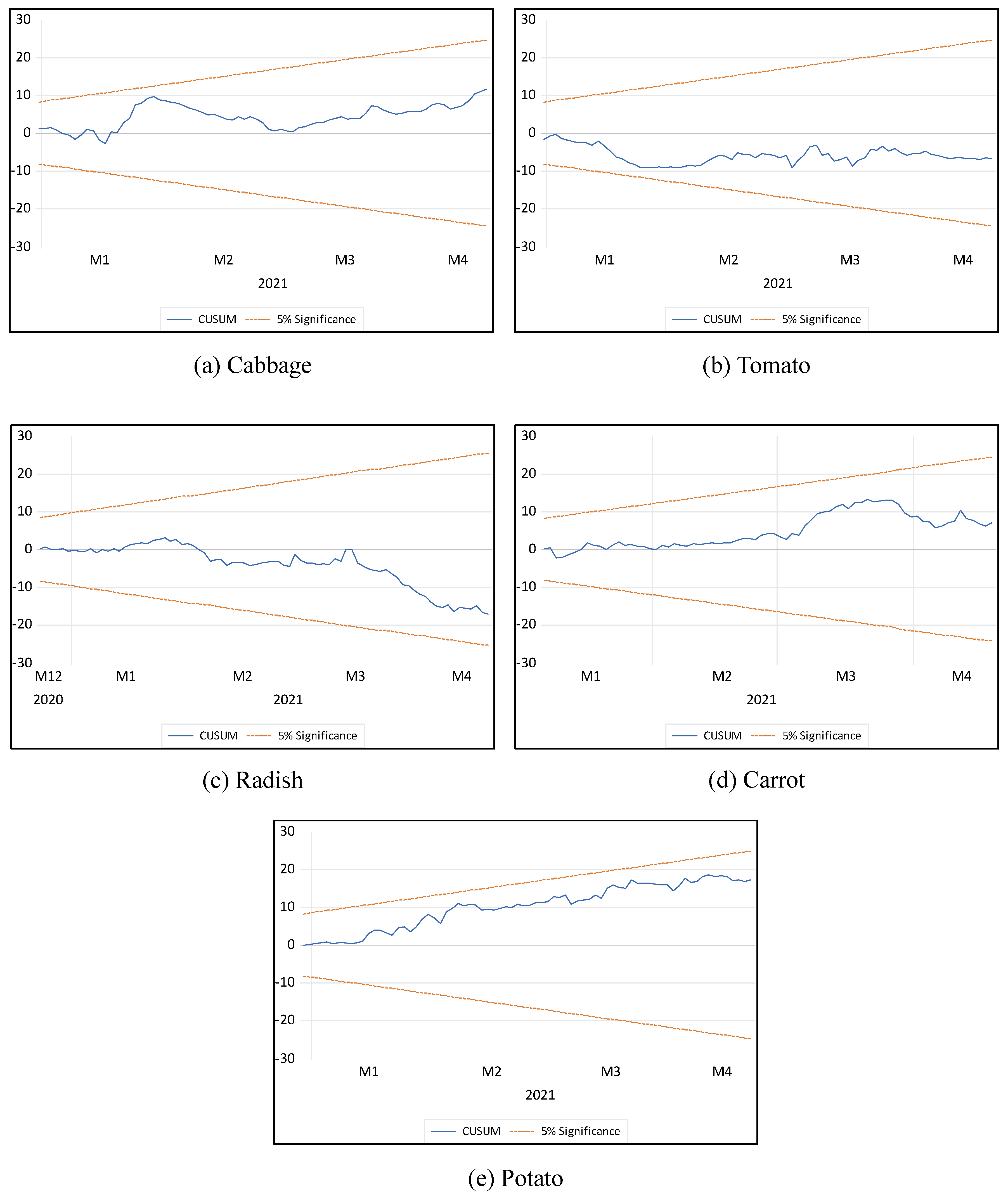
Appendix A. ARDL Cumulative Sum (CUSUM) Test for Stability


References
- Hadjidemetriou, G.M.; Sasidharan, M.; Kouyialis, G.; Parlikad, A.K. The impact of government measures and human mobility trend on COVID-19 related deaths in the UK. Transp. Res. Interdiscip. Perspect. 2020, 6, 100167. [Google Scholar] [CrossRef] [PubMed]
- Tison, G.H.; Avram, R.; Kuhar, P.; Abreau, S.; Marcus, G.M.; Pletcher, M.J.; Olgin, J.E. Worldwide effect of COVID-19 on physical activity: A descriptive study. Ann. Intern. Med. 2020, 173, 767–770. [Google Scholar] [CrossRef] [PubMed]
- Alam, G.M.M.; Khatun, M.N. Impact of COVID-19 on vegetable supply chain and food security: Empirical evidence from Bangladesh. PLoS ONE 2021, 16, e0248120. [Google Scholar] [CrossRef] [PubMed]
- Richards, T.J.; Rickard, B. COVID-19 impact on fruit and vegetable markets. Can. J. Agric. Econ. 2020, 68, 189–194. [Google Scholar] [CrossRef]
- Singh, S.; Kumar, R.; Panchal, R.; Tiwari, M.K. Impact of COVID-19 on logistics systems and disruptions in food supply chain. Int. J. Prod. Res. 2021, 59, 1993–2008. [Google Scholar] [CrossRef]
- Deaton, B.J.; Deaton, B.J. Food security and Canada’s agricultural system challenged by COVID-19. Can. J. Agric. Econ. 2020, 68, 143–149. [Google Scholar] [CrossRef]
- Reddy, V.R.; Singh, S.K.; Anbumozhi, S. Food Supply Chain Disruption due to National Disasters: Entities, Risks, and Strategies for Resilience; ERIA Discussion Paper Series; Economic Research Institute for ASEAN and Asia: Jakarta, Indonesia, 2016. [Google Scholar]
- Chari, F.; Muzinda, O.; Novukela, C.; Ngcamu, B.S. Pandemic outbreaks and food supply chains in developing countries: A case of COVID-19 in Zimbabwe. Cogent Bus. Manag. 2022, 9, 2026188. [Google Scholar] [CrossRef]
- USDA, COVID-19 Impacts on Food Distribution in Japan-Update II, 2020. Available online: https://apps.fas.usda.gov/newgainapi/api/Report/DownloadReportByFileName?fileName=COVID-19%20Impacts%20on%20Food%20Distribution%20in%20Japan%20-%20Update%20II_Tokyo%20ATO_Japan_05-26-2020 (accessed on 23 June 2021).
- IMF. International Monetary Fund. World Economic Outlook Update, June 2020. Available online: https://www.imf.org/en/Publications/WEO/Issues/2020/06/24/WEOUpdateJune2020 (accessed on 23 June 2021).
- Lichten, J.; Kondo, C. Resilient Japanese local food systems thrive during COVID-19: Ten groups, ten outcomes. This article is a part of The Special Issue: Vulnerable Populations Under COVID-19 in Japan. Aisa-Pac. J. 2020, 18. Available online: https://apjjf.org/2020/18/Kondo-Lichten.html (accessed on 22 February 2022).
- Islam, M.M.; Jannat, A.; Al Rafi, D.A.; Aruga, K. Potential economic impacts of the COVID-19 pandemic on South Asian economies: A review. World 2020, 1, 283–299. [Google Scholar] [CrossRef]
- Nickle, A. Retail Produce Sales Rising Amid Coronavirus Concerns. The Packer. 2020. Available online: https://www.thepacker.com/article/retail-produce-sales-rising-amid-coronavirus-concerns? (accessed on 25 April 2021).
- Aruga, K.; Islam, M.M.; Jannat, A. Does Staying at Home during the COVID-19 Pandemic Help Reduce CO2 Emissions? Sustainability 2021, 13, 8534. [Google Scholar] [CrossRef]
- Jena, P.R.; Kalli, R.; Tanti, P.C. Impact of COVID-19 on Agricultural System and Food Prices: The Case of India. In Rural Health; IntechOpen: London, UK, 2021. [Google Scholar] [CrossRef]
- Chen, J.; Yang, C.-C. How COVID-19 Affects Agricultural Food Sales: Based on the Perspective of China’s Agricultural Listed Companies’ Financial Statements. Agriculture 2021, 11, 1285. [Google Scholar] [CrossRef]
- Reardon, T.; Bellemare, M.F.; Zilberman, D. How COVID-19 May Disrupt Food Supply Chains in Developing Countries. IFPRI Book Chapters: 2020, 78–80. Available online: https://www.ifpri.org/blog/how-covid-19-may-disrupt-food-supply-chains-developing-countries (accessed on 7 March 2022).
- Akter, S. The impact of COVID-19 related ‘stay-at-home’ restrictions on food prices in Europe: Findings from a preliminary analysis. Food Secur. 2020, 12, 719–725. [Google Scholar] [CrossRef] [PubMed]
- World Population Review. Japan Population, 2022 (Live). Available online: https://worldpopulationreview.com/countries/japan-population (accessed on 22 February 2022).
- Statista. Most Commonly Eaten Fruits and Vegetables in Japan as of November. 2020. Available online: https://www.statista.com/statistics/1229250/japan-most-eaten-fruit/ (accessed on 23 June 2021).
- Kohls, R.L. Marketing of Agricultural Products, 9th ed.; Prentice Hall: Upper Saddle River, NJ, USA, 2002. [Google Scholar]
- Metropolitan Central Wholesale Market (MCWM). Metropolitan Central Wholesale Market Daily Report. 2022. Available online: https://www.shijou-nippo.metro.tokyo.lg.jp/index.html (accessed on 9 February 2022).
- Google LLC. Google COVID-19 Community Mobility Reports. Available online: https://www.google.com/covid19/mobility/ (accessed on 6 February 2021).
- Phillips, P.C.; Perron, P. Testing for a unit root in time series regression. Biometrika 1988, 75, 335–346. [Google Scholar] [CrossRef]
- Dickey, D.A.; Fuller, W.A. Distribution of the estimators for autoregressive time series with a unit root. J Am. Stat. Assoc. 1979, 74, 427–431. [Google Scholar]
- Kwiatkowski, D.; Phillips, P.C.; Schmidt, P.; Shin, Y. Testing the null hypothesis of stationarity against the alternative of a unit root: How sure are we that economic time series have a unit root? J. Econom. 1992, 54, 159–178. [Google Scholar] [CrossRef]
- Pesaran, M.H.; Shin, Y.; Smith, R.J. Bounds testing approaches to the analysis of level relationships. J. Appl. Econ. 2001, 16, 289–326. [Google Scholar] [CrossRef]
- Nyga-Łukaszewska, H.; Aruga, K. Energy prices, and COVID-immunity: The case of crude oil and natural gas prices in the US and Japan. Energies 2020, 13, 6300. [Google Scholar] [CrossRef]
- Breusch, T.S. Testing for Autocorrelation in Dynamic Linear Models. Aust. Econ. Pap. 1978, 17, 334–355. [Google Scholar] [CrossRef]
- Godfrey, L.G. Testing against general autoregressive and moving average error models when the regressors include lagged dependent variables. Econometrica 1978, 46, 1293. [Google Scholar] [CrossRef]
- Breusch, T.S.; Pagan, A.R. A simple test for heteroscedasticity and random coefficient variation. Econometrica 1979, 47, 1287. [Google Scholar] [CrossRef]
- Sudha, N.; Shree, S. Urban Food Markets and the Lockdown in India. 2020. Available online: https://doi.org/10.2139/ssrn.3599102 (accessed on 23 June 2021).

| Variables | Symbol | Measurement Unit | Sources |
|---|---|---|---|
| Cabbage price | CP | 10 pieces (JPY) | Toyosu market [22] |
| Cabbage volume | CV | Kg | |
| Tomato price | TP | 4 pieces (JPY) | |
| Tomato volume | TV | Kg | |
| Radish price | RP | 10 pieces (JPY) | |
| Radish volume | RV | Kg | |
| Carrot price | CRP | 10 Pieces (JPY) | |
| Carrot volume | CRV | Kg | |
| Potato price | PP | 10 pieces (JPY) | |
| Potato volume | PV | Kg | |
| Residential (stay-at-home restriction index) | Home | The number of visitors to residential areas has changed compared to baseline days (the median value for the 5 weeks from 3 January to 6 February 2020). This index is smoothed to a rolling 7-day average. | Google LLC [23] |
| COVID-19 cases in Tokyo | TC | Daily (Number) | https://stopcovid19.metro.tokyo.lg.jp (accessed on 25 February 2022) |
| SOEs | Starting Dates | Ending Dates | Before 4 Weeks | After 4 Weeks |
|---|---|---|---|---|
| 1st | 7 April 2020 | 25 May 2020 | 10 March 2020 | 22 June 2020 |
| 2nd | 8 January 2021 | 21 March 2021 | 11 December 2020 | 17 April 2021 |
| 3rd | 25 April 2021 | 20 June 2021 | 29 March 2021 | 17 July 2021 |
| 4th | 2 July 2021 | 30 September 2021 | 14 June 2021 | 28 October 2021 |
| SOE | Variables | Levels | First Differences | ||||
|---|---|---|---|---|---|---|---|
| PP | ADF | KPSS | PP | ADF | KPSS | ||
| 1st | CP | −2.514 | −2.973 | 0.205 ** | −7.561 *** | −7.603 *** | 0.032 |
| CV | −7.537 *** | −4.420 *** | 0.154 ** | −41.412 *** | −7.315 *** | 0.162 ** | |
| TP | −2.983 | −1.184 | 0.186 ** | −15.217 *** | −14.974 *** | 0.110 | |
| TV | −10.827 *** | −2.490 | 0.092 | −29.397 *** | −8.483 *** | 0.050 | |
| RP | −5.405 *** | −5.124 *** | 0.062 | −13.188 *** | −9.300 *** | 0.048 | |
| RV | −5.818 *** | −2.961 ** | 0.284 *** | −68.237 *** | −4.885 *** | 0.175 ** | |
| CRP | −5.327 *** | −1.658 | 0.202 ** | −18.654 *** | −4.936 *** | 0.044 | |
| CRV | −8.585 *** | −2.672 | 0.234 *** | −39.507 *** | −4.959 *** | 0.007 | |
| PP | −5.356 *** | −5.315 *** | 0.102 | −29.271 *** | −7.162 *** | 0.075 | |
| PV | −8.039 *** | −8.041 *** | 0.103 | −35.333 *** | −8.146 *** | 0.252 *** | |
| Home | −0.802 | −1.134 | 0.262 *** | −5.137 *** | −5.107 *** | 0.096 | |
| TC | −2.738 | −3.130 | 0.188 ** | −16.59 *** | −1.471 | 0.178 ** | |
| 2nd | CP | −3.965 ** | −3.681 ** | 0.099 | −13.483 *** | −6.886 *** | 0.130 * |
| CV | −8.131 *** | −8.127 *** | 0.049 | −65.965 *** | −8.373 *** | 0.088 | |
| TP | −7.060 *** | −2.483 | 0.258 *** | −35.331 *** | −7.537 *** | 0.048 | |
| TV | −9.634 *** | −9.628 *** | 0.079 | −37.267 *** | −5.114 *** | 0.021 | |
| RP | −3.022 | −2.687 | 0.221 *** | −12.682 *** | −4.549 *** | 0.032 | |
| RV | −9.552 *** | −3.302 * | 0.055 | −19.674 *** | −7.923 *** | 0.069 | |
| CRP | −4.708 *** | −1.890 | 0.188 ** | −17.683 *** | −11.029 *** | 0.020 | |
| CRV | −7.467 *** | −1.595 | 0.314 *** | −38.190 *** | −5.592 *** | 0.188 ** | |
| PP | −7.651 *** | −6.713 *** | 0.217 *** | −34.202 *** | −6.183 *** | 0.127 * | |
| PV | −8.405 *** | −8.407 *** | 0.061 | −35.075 *** | −7.325 *** | 0.093 | |
| Home | −3.528 ** | −3.610 ** | 0.142 * | −12.383 *** | −8.073 *** | 0.111 | |
| TC | −3.035 | −2.788 | 0.133 * | −11.769 *** | −2.529 | 0.145 * | |
| 3rd | CP | −2.993 | −3.211 * | 0.081 | −7.768 *** | −7.744 *** | 0.047 |
| CV | −5.222 *** | −1.749 | 0.247 *** | −24.693 *** | −10.538 *** | 0.168 ** | |
| TP | −5.149 *** | 2.918 | 0.197 ** | −18.165 *** | −4.891 *** | 0.031 | |
| TV | −8.773 *** | −2.541 | 0.100 | −18.105 *** | −4.688 *** | 0.058 | |
| RP | −4.051 ** | −2.490 | 0.106 | −14.108 *** | −5.285 *** | 0.056 | |
| RV | −4.686 *** | −2.357 | 0.235 *** | −27.279 *** | −2.188 | 0.229 *** | |
| CRP | −5.535 *** | −5.561 *** | 0.156 ** | −24.510 *** | −8.155 *** | 0.182 ** | |
| CRV | −9.974 *** | −5.462 *** | 0.098 | −46.317 *** | −9.900 *** | 0.111 | |
| PP | −4.118 *** | −3.423 * | 0.260 *** | −20.285 *** | −6.126 *** | 0.095 | |
| PV | −8.358 *** | −2.191 | 0.230 *** | −48.691 *** | −4.196 *** | 0.099 | |
| Home | −2.451 | −2.158 | 0.176 ** | −5.317 *** | −5.845 *** | 0.033 | |
| TC | −3.390 * | −0.627 | 0.179 ** | −13.742 *** | −0.627 | 0.500 *** | |
| 4th | CP | −2.165 | −1.873 | 0.146 ** | −12.077 *** | 12.077 *** | 0.068 |
| CV | −7.977 *** | −3.600 ** | 0.212 ** | −25.953 *** | −8.437 *** | 0.094 | |
| TP | −2.760 | −1.954 | 0.129* | −16.117 *** | −16.753 *** | 0.030 | |
| TV | −8.194 *** | −1.631 | 0.231 *** | −48.256 *** | −5.033 *** | 0.138 * | |
| RP | −5.681 *** | −3.411 * | 0.083 | −15.651 *** | −5.634 *** | 0.049 | |
| RV | −7.778 *** | −4.084 *** | 0.239 *** | −35.492 *** | −9.030 *** | 0.132 * | |
| CRP | −9.803 *** | −3.574 ** | 0.163 ** | −43.892 *** | −12.969 *** | 0.082 | |
| CRV | −9.949 *** | −2.071 | 0.200 ** | −46.269 | −10.873 *** | 0.453 *** | |
| PP | −8.186 *** | −3.396 * | 0.179 ** | −28.233 *** | −9.124 *** | 0.085 | |
| PV | −8.306 *** | −8.306 *** | 0.285 *** | −37.750 *** | −8.980 *** | 0.157 ** | |
| Home | −2.037 | −0.280 | 0.258 *** | −7.629 *** | −3.262 * | 0.034 | |
| TC | −1.577 | −2.290 | 0.261 *** | −14.362 *** | −1.867 | 0.096 | |
| SOE | Model | BG F-Stat. | BPG F-Stat. | SOE | Model | BG F-Stat. | BPG F-Stat. |
|---|---|---|---|---|---|---|---|
| 1st | Cabbage | 0.085 | 2.668 ** | Cabbage | 0.711 | 0.668 | |
| Tomato | 2.803 * | 1.361 | Tomato | 0.658 | 3.565 *** | ||
| Radish | 0.634 | 0.807 | 3rd | Radish | 1.307 | 1.504 | |
| Carrot | 1.127 | 3.485 *** | Carrot | 0.482 | 4.319 *** | ||
| Potato | 1.598 | 0.290 | Potato | 0.426 | 0.854 | ||
| 2nd | Cabbage | 1.803 | 1.860 * | Cabbage | 0.226 | 1.681 | |
| Tomato | 0.184 | 1.530 | Tomato | 4.236 ** | 0.879 | ||
| Radish | 0.549 | 2.119 * | 4th | Radish | 1.696 | 1.691 * | |
| Carrot | 1.043 | 2.746 *** | Carrot | 0.399 | 2.140 ** | ||
| Potato | 1.618 | 1.002 | Potato | 0.019 | 0.937 |
| SOE | Statistics | CP | CV | TP | TV | RP | RV | CRP | CRV | PP | PV | Home | TC |
|---|---|---|---|---|---|---|---|---|---|---|---|---|---|
| 1st | Mean | 1230.9 | 74,509.5 | 1215.8 | 36,446.5 | 907.6 | 20,738.3 | 1423.4 | 62,811.2 | 1718.9 | 23,965.9 | 9.8 | 56.6 |
| Median | 1107 | 71,001 | 1215 | 33,838 | 936.0 | 19,528.5 | 1476.0 | 50,793.0 | 1566 | 21,964 | 8.8 | 28.5 | |
| Maximum | 3276 | 125,340 | 2088 | 73,050 | 1515.7 | 39,350.0 | 2079.0 | 214,271.0 | 3240 | 53,630 | 21.1 | 204 | |
| Minimum | 684 | 44,060 | 576 | 15076 | 360.0 | 9145.0 | 468.0 | 3864.0 | 720 | 6636 | 3.4 | 0 | |
| Std. Dev. | 495.8 | 18,489.8 | 453.7 | 13,285.2 | 311.3 | 6693.8 | 333.9 | 39,205.0 | 700.5 | 9688.7 | 4.4 | 59.2 | |
| Skewness | 1.99 | 0.59 | 0.275 | 0.741 | −0.01 | 0.76 | −0.41 | 1.47 | 0.633 | 0.814 | 0.612 | 1.1 | |
| Kurtosis | 7.59 | 2.74 | 1.64 | 3.35 | 1.97 | 3.02 | 3.11 | 5.35 | 2.41 | 3.86 | 2.66 | 3 | |
| Jarque–Bera | 114.1 *** | 4.5 | 6.6 ** | 7.2 ** | 3.3 | 7.0 ** | 2.1 | 43.9 *** | 6.0 ** | 10.5 *** | 5.0 * | 16.1 *** | |
| Obs. | 74 | 74 | 74 | 74 | 74 | 74 | 74 | 74 | 74 | 74 | 74 | 74 | |
| 2nd | Mean | 703.3 | 75,165.7 | 1135.8 | 30,285.4 | 728.3 | 31,151.9 | 1486.2 | 52,352.9 | 1715.2 | 23,036 | 6.6 | 651 |
| Median | 666 | 73,485 | 1152 | 28,497.5 | 780.7 | 30,262.5 | 1469.7 | 44,562.0 | 1746 | 21,249.5 | 5.9 | 451.5 | |
| Maximum | 1188 | 119,982 | 1476 | 85,952 | 1260.0 | 75,545.0 | 2340.0 | 16,6562.0 | 3276 | 80,370 | 18.5 | 2520 | |
| Minimum | 441 | 33,708 | 684 | 14286 | 180.0 | 12,015.0 | 648.0 | 19,896.0 | 486 | 1401 | 4 | 116 | |
| Std. Dev. | 164.1 | 19,726.98 | 168 | 10,884.9 | 257.3 | 9346.8 | 390.9 | 27,128.2 | 614.3 | 11,657.3 | 2.2 | 514.7 | |
| Skewness | 0.98 | 0.174164 | −0.21 | 1.76 | −0.32 | 1.48 | 0.40 | 1.93 | 0.12 | 1.51 | 2.25 | 1.92 | |
| Kurtosis | 3.53 | 2.38526 | 2.79 | 9.3 | 2.49 | 8.19 | 2.61 | 7.35 | 2.94 | 8.23 | 11.01 | 6.6 | |
| Jarque–Bera | 15.4 *** | 1.8 | 0.83 | 191.2 *** | 2.4 | 130.7 *** | 2.9 | 124.0 *** | 0.2 | 134.3 *** | 310.1 *** | 100.7 *** | |
| Obs. | 88 | 88 | 88 | 88 | 88 | 88 | 88 | 88 | 88 | 88 | 88 | 88 | |
| 3rd | Mean | 731.8 | 78,812.7 | 1093.4 | 36,420.2 | 730.3 | 19,051.1 | 1099.2 | 53,344.8 | 2010.2 | 19,599.3 | 6.2 | 610.4 |
| Median | 702 | 76,569 | 1116 | 32,783 | 630.0 | 18,165.0 | 1044.0 | 47,393.0 | 1980 | 19,700 | 6 | 563 | |
| Maximum | 1188 | 128,977 | 1836 | 84,185 | 1512.0 | 33,236.0 | 2916.0 | 166,562.0 | 3456 | 41,576 | 12.8 | 1411 | |
| Minimum | 450 | 43,238 | 432 | 15,574 | 180.0 | 10,365.0 | 684.0 | 25,951.0 | 756 | 1401 | 4 | 208 | |
| Std. Dev. | 186.9 | 20,078.8 | 247.6 | 13,048.1 | 379.9 | 5202.8 | 333.4 | 26,860.3 | 758.9 | 7419.3 | 1.8 | 257.3 | |
| Skewness | 0.54 | 0.47 | 0.56 | 0.99 | 0.30 | 0.71 | 2.60 | 2.08 | 0.03 | 0.12 | 2.16 | 0.86 | |
| Kurtosis | 2.33 | 2.67 | 4.11 | 4.03 | 1.82 | 3.23 | 13.19 | 7.49 | 1.96 | 3.05 | 8.16 | 3.62 | |
| Jarque–Bera | 5.4 * | 3.3 | 8.4 ** | 16.5 *** | 5.7 ** | 6.9 ** | 430.8 *** | 123.1 *** | 3.6 | 0.2 | 149.7 *** | 11.0 *** | |
| Obs. | 79 | 79 | 79 | 79 | 79 | 79 | 79 | 79 | 79 | 79 | 79 | 79 | |
| 4th | Mean | 855 | 98,663.6 | 1488.9 | 43,845.3 | 1018.2 | 26,736.4 | 955.8 | 54,780.2 | 1224.6 | 19,086.3 | 6.8 | 1513.4 |
| Median | 828 | 95,145 | 1404 | 39,238 | 1026.0 | 24,583.0 | 900.0 | 51,241.0 | 1080 | 18,534 | 6.1 | 715 | |
| Maximum | 1368 | 157,686 | 2520 | 121,453 | 1341.0 | 57,390.0 | 2646.0 | 112,927.0 | 2170.2 | 42,992 | 12.5 | 5908 | |
| Minimum | 396 | 51,458 | 432 | 14,103 | 648.0 | 12,225.0 | 252.0 | 7573.0 | 504 | 2870 | 4.2 | 14 | |
| Std. Dev. | 249.2 | 20,000.9 | 463.8 | 19,703.3 | 144.6 | 9783.2 | 403.3 | 24,005.3 | 411.3 | 8727.1 | 1.7 | 1700.6 | |
| Skewness | 0.43 | 0.41 | 0.4 | 1.23 | -0.32 | 0.85 | 1.29 | 0.39 | 0.46 | 0.65 | 0.91 | 1.15 | |
| Kurtosis | 2.68 | 3.04 | 2.54 | 5.21 | 2.58 | 3.24 | 5.78 | 2.36 | 2.26 | 3.28 | 3.58 | 3.01 | |
| Jarque–Bera | 3.4 | 2.7 | 3.4 | 43.6 *** | 2.3 | 11.7 *** | 57.0 *** | 4.1 | 5.6 * | 7.1 ** | 14.7 *** | 21.1 *** | |
| Obs. | 95 | 95 | 95 | 95 | 95 | 95 | 95 | 95 | 95 | 95 | 95 | 95 |
| SOE | Model | F-Stat. | SOE | Model | F-Stat. |
|---|---|---|---|---|---|
| 1st | Cabbage | 5.012 ** | Cabbage | 4.110 ** | |
| Tomato | 7.873 *** | Tomato | 4.720 ** | ||
| Radish | 5.067 ** | 3rd | Radish | 4.027 ** | |
| Carrot | 5.155 ** | Carrot | 11.075 *** | ||
| Potato | 0.513 | Potato | 1.533 | ||
| 2nd | Cabbage | 10.244 *** | 4th | Cabbage | 4.211 ** |
| Tomato | 1.854 | Tomato | 4.313 ** | ||
| Radish | 2.043 | Radish | 3.239 | ||
| Carrot | 2.161 | Carrot | 1.718 | ||
| Potato | 11.911 *** | Potato | 5.660 *** |
| SOE | Model | Variable | Coefficient | Std. Error | SOE | Model | Variable | Coefficient | Std. Error |
|---|---|---|---|---|---|---|---|---|---|
| 1st | Cabbage | CV | −0.017 *** | 0.006 | 3rd | Cabbage | CV | −0.005 | 0.004 |
| Home | 13.757 | 29.518 | Home | −84.296 ** | 37.099 | ||||
| Intercept | 2160.218 *** | 558.716 | Intercept | 1682.096 *** | 562.853 | ||||
| Tomato | TV | −0.045 *** | 0.000 | Tomato | TV | −0.018 * | 0.010 | ||
| Home | −33.779 *** | 18.925 | Home | −8.624 | 25.269 | ||||
| Intercept | 3255.134 *** | 200.373 | Intercept | 1397.284 *** | 284.123 | ||||
| Radish | RV | −0.059 *** | 0.016 | Radish | RV | −0.086 *** | 0.030 | ||
| Home | −49.566 *** | 19.489 | Home | −151.611 ** | 70.569 | ||||
| Intercept | 2656.195 *** | 507.184 | Intercept | 3316.003 *** | 838.832 | ||||
| Carrot | CRV | 0.002 * | 0.001 | Carrot | CRV | 0.009 *** | 0.001 | ||
| Home | −23.747 ** | 9.825 | Home | 41.863 *** | 15.054 | ||||
| Intercept | 1656.536 *** | 121.651 | Intercept | 72.237 | 122.383 | ||||
| Potato | PV | 0.009 | 0.090 | Potato | PV | 1.668 | 14.053 | ||
| Home | 12.450 | 114.869 | Home | 925.044 | 6162.287 | ||||
| Intercept | 2303.873 | 2521.096 | Intercept | −19,670.67 | 172,079.6 | ||||
| 2nd | Cabbage | CV | −0.004 * | 0.002 | 4th | Cabbage | CV | −0.004 | 0.004 |
| Home | −22.739 | 17.277 | Home | 161.634 *** | 36.135 | ||||
| Intercept | 1007.155 *** | 214.296 | Intercept | 312.410 | 436.952 | ||||
| Tomato | TV | −0.005 | 0.007 | Tomato | TV | −0.043 ** | 0.021 | ||
| Home | −58.349 *** | 21.914 | Home | 235.752 ** | 117.570 | ||||
| Intercept | 1600.767 *** | 246.093 | Intercept | 1626.512 ** | 708.625 | ||||
| Radish | RV | 0.010 | 0.010 | Radish | RV | −0.002 | 0.004 | ||
| Home | 94.652 ** | 48.262 | Home | 37.638 * | 22.480 | ||||
| Intercept | −96.643 | 341.573 | Intercept | 841.351 *** | 176.901 | ||||
| Carrot | CRV | −0.013 ** | 0.007 | Carrot | CRV | −0.004 | 0.005 | ||
| Home | −1.388 | 69.859 | Home | −55.053 | 90.745 | ||||
| Intercept | 2242.169 *** | 628.082 | Intercept | 1563.857 *** | 545.154 | ||||
| Potato | PV | −0.033 *** | 0.008 | Potato | PV | 0.017 ** | 0.009 | ||
| Home | 48.624 | 43.376 | Home | 99.069 ** | 42.242 | ||||
| Intercept | 2361.682 *** | 289.082 | Intercept | 384.390 | 257.764 |
| SOE | Model | Variable | Coefficient | Std. Error | SOE | Model | Variable | Coefficient | Std. Error |
|---|---|---|---|---|---|---|---|---|---|
| 1st | Cabbage | ΔCV | −0.005 *** | 0.002 | 3rd | Cabbage | ΔCV | −0.002 ** | 0.001 |
| ΔHome | 4.182 | 9.027 | ΔHome | −18.237 ** | 7.269 | ||||
| TC | 0.921 | 0.594 | TC | −0.003 | 0.045 | ||||
| Tomato | ΔTV | −0.003 * | 0.001 | Tomato | ΔTV | −0.001 | 0.002 | ||
| ΔHome | 32.592 * | 19.536 | ΔHome | −3.407 | 13.601 | ||||
| TC | −0.835 *** | 0.296 | TC | 0.264 *** | 0.096 | ||||
| Radish | ΔRV | 0.0008 | 0.006 | Radish | ΔRV | 0.008 * | 0.005 | ||
| ΔHome | −22.253 *** | 8.320 | ΔHome | −27.445 ** | 10.942 | ||||
| TC | −0.156 | 0.450 | TC | 0.028 | 0.076 | ||||
| Carrot | ΔCRV | 0.001 ** | 0.001 | Carrot | ΔCRV | 0.004 *** | 0.001 | ||
| ΔHome | −102.695 *** | 42.216 | ΔHome | −56.650 | 47.224 | ||||
| TC | −1.994 *** | 0.695 | TC | 0.490 *** | 0.134 | ||||
| Potato | ΔPV | 0.001 | 0.004 | Potato | ΔPV | 0.006 | 0.008 | ||
| ΔHome | 0.792 | 9.654 | ΔHome | −10.528 | 38.373 | ||||
| TC | −0.234 | 0.739 | TC | 0.259 | 0.253 | ||||
| 2nd | Cabbage | ΔCV | −0.001 | 0.001 | 4th | Cabbage | ΔCV | 0.001 | 0.001 |
| ΔHome | 9.784 | 8.039 | ΔHome | 10.91 | 17.682 | ||||
| TC | 0.083 ** | 0.035 | TC | −0.020 ** | 0.01 | ||||
| Tomato | ΔTV | 0.001 | 0.002 | Tomato | ΔTV | −0.004 *** | 0.001 | ||
| ΔHome | −24.08 | 12.079 | ΔHome | 23.314 | 17.243 | ||||
| TC | 0.028 | 0.047 | TC | 0.014 | 0.019 | ||||
| Radish | ΔRV | 0.002 | 0.001 | Radish | ΔRV | −0.004 * | 0.002 | ||
| ΔHome | 16.879 * | 9.861 | ΔHome | 13.901 * | 8.374 | ||||
| TC | −0.040 | 0.034 | TC | −0.003 | 0.009 | ||||
| Carrot | ΔCRV | 0.001 | 0.001 | Carrot | ΔCRV | 0.003 | 0.002 | ||
| ΔHome | −0.410 | 20.639 | ΔHome | −22.761 | 32.721 | ||||
| TC | −0.016 | 0.085 | TC | 0.005 | 0.034 | ||||
| Potato | ΔPV | 0.008 | 0.005 | Potato | ΔPV | 0.010 ** | 0.004 | ||
| ΔHome | 34.767 | 32.753 | ΔHome | −31.954 | 53.664 | ||||
| TC | −0.204 | 0.147 | TC | −0.076 ** | 0.034 |
Publisher’s Note: MDPI stays neutral with regard to jurisdictional claims in published maps and institutional affiliations. |
© 2022 by the authors. Licensee MDPI, Basel, Switzerland. This article is an open access article distributed under the terms and conditions of the Creative Commons Attribution (CC BY) license (https://creativecommons.org/licenses/by/4.0/).
Share and Cite
Aruga, K.; Islam, M.M.; Jannat, A. Effects of the State of Emergency during the COVID-19 Pandemic on Tokyo Vegetable Markets. Sustainability 2022, 14, 9719. https://doi.org/10.3390/su14159719
Aruga K, Islam MM, Jannat A. Effects of the State of Emergency during the COVID-19 Pandemic on Tokyo Vegetable Markets. Sustainability. 2022; 14(15):9719. https://doi.org/10.3390/su14159719
Chicago/Turabian StyleAruga, Kentaka, Md. Monirul Islam, and Arifa Jannat. 2022. "Effects of the State of Emergency during the COVID-19 Pandemic on Tokyo Vegetable Markets" Sustainability 14, no. 15: 9719. https://doi.org/10.3390/su14159719
APA StyleAruga, K., Islam, M. M., & Jannat, A. (2022). Effects of the State of Emergency during the COVID-19 Pandemic on Tokyo Vegetable Markets. Sustainability, 14(15), 9719. https://doi.org/10.3390/su14159719