Optimal Speed Model of Urban Underwater Tunnel Based on CO₂ Emissions Factor

Abstract

This study aims to reduce air pollution caused by vehicle emissions in confined spaces and realize low-carbon travel in urban underwater tunnels. Based on the MEET (Methodologies for Estimating Air Pollutant Emissions from Transport) and COPERT (Computer Programme to Calculate Emissions from Road Transport) models, combined with real vehicle test data, an urban underwater tunnel speed–CO₂ emissions factor model was constructed. Results show that: Different working conditions have a great impact on the MEET model; load and slope factors expand the actual CO₂ emissions factor, which is different from the actual situation. The CO₂ emissions factor in the COPERT model is negatively correlated with the speed, and there are fewer variables in the model, so the parameters are more controllable and more in line with the actual situation. According to the vehicle gasoline consumption and taking CO_{2, i} > GC as the judgment index, the optimal limit speed of the ramp is calculated to be 40 km/h, while the main line maintains the existing state of 60 km/h. The model is simple and easy to operate, can be applied to estimate vehicle CO₂ emissions factor at underwater tunnels in other cities, providing a basis for traffic management and effectively realizing low-carbon travel.

1. Introduction

In response to pollution, global warming, and other environmental issues, countries worldwide are actively exploring energy conservation and emission reduction measures, specifically concerning the transportation industry. To effectively control carbon emissions generated by fueled vehicles, the public has become increasingly interested in vehicles that run on alternative energy sources. However, as most vehicles currently run on gasoline, controlling the carbon emissions of existing, gasoline-fueled, vehicles remains a pressing issue today. The calculation results of carbon emissions can arouse people’s attention to the pollutants emitted in transportation, so as to seek a green and environmental protection mode of transportation and achieve the purpose of improving the road traffic environment. Vicente et al. reviewed the development process of measurement methods for related carbon emission factors [1]. Wang et al. proposed a fuel-saving, emission-reduction strategy for signalized intersections, starting from the bounded rationality and speed guidance of drivers [2]. Hyung-Wook et al. estimated the carbon emissions of vehicles at constant and variable speeds [3]. Zhang et al. determined the best velocity resolution by tuning and calibrating the time to improve emission estimates [4]. Or compare the changes in carbon emissions of different types of vehicles after changing the fuel mode [5,6,7]. Ashik et al. investigated whether transit-oriented development (TOD) has an impact on the CO₂ emissions from residents’ travel [8]. These studies focus mainly on the evaluation of the overall carbon emissions in investigated cities and the planning of optimal routes for public transportation. While productive, these concepts are macroscopic and serve to reduce carbon emissions, achieve environmental improvement, or compare specific vehicle emissions. For the relevant influencing factors involved in carbon emissions, such as speed, the research objects focused on highways and urban expressways.

The urban underwater tunnel, a road built to meet the needs of cities along the river and sea, has become part of the daily commute for people along the river coast. The goal of optimizing the driving environment of today’s urban underwater tunnels is to increase driving comfort while ensuring driving safety and reducing air pollution caused by vehicle emissions in confined spaces. Jiao et al. studied the reasonable length of the entrance area of a subsea tunnel based on the visual characteristics of drivers [9], and, at the same time, started from speed perception, constructed different visual reference systems, and proposed tunnel optimization facilities [10]. Yang et al. analyzed the correlation between EEG (electroencephalography) data and the speed of undersea tunnel drivers [11]. However, there have been no studies on the optimal driving speed and carbon emissions in urban underwater tunnels. Therefore, this study’s starting point was to find out what speed was necessary for the vehicle, with the highest proportion of urban travel, utilizing underwater tunnels, to achieve the best environmental improvement state among various models.

By summarizing and comparing existing carbon emission-velocity models, this study constructs a speed–CO₂ emissions factor model for urban underwater tunnels and calculates the optimal velocity at the urban underwater tunnel ramp and mainline. This provides a basis for traffic management in urban underwater tunnels and maximization of low-carbon travel. This study was based on the MEET and COPERT models. The first step was to introduce the source of the model, equations used to estimate the model, definition of various parameters, and application of existing research to the model. The second step was to obtain relevant data through real vehicle tests, such as speed, and incorporate them into different models to calculate the CO₂ emissions factor of urban underwater tunnels. Through comparison, we chose the CO₂ emission calculation model that is most suitable for this study. The third step was to obtain a fitting model through the correlation between speed and CO₂ emissions factor and determine the final optimal driving speed according to gasoline consumption.

The driving characteristics of motorists were analyzed based on behavior in urban underwater tunnels. The urban underwater tunnel CO₂ emissions factor model, with speed as a variable, can be applied to the estimation of underwater tunnel CO₂ emissions factor at any known driving speed. Furthermore, the optimal speed limit value is determined by the relative relationship between gasoline consumption and CO₂ emissions factor, and this type of process can be used for further development of models with other variables as the main parameter.

2. Basic Model of Velocity and Emissions

‘Vehicle emissions’ refers to various types of greenhouse gases, such as carbon dioxide (CO₂), nitrogen oxides (NO_x), and sulfur dioxide (SO₂), which are produced by fuel combustion. Relevant studies have proposed various emission models such as MEET (Methodologies for Estimating Air Pollutant Emissions from Transport), ETW (EcoTransIT World), COPERT (Computer Programme to Calculate Emissions from Road Transport), MOBILE (Mobile Source Emission Factor Model), and MOVES (Motor Vehicle Emissions Simulator). Starting from the calculation parameters of different models, the scope of application of the above models is summarized. The MOBILE emphasizes the relationship between mileage and emissions [12]. The MOVES stores the basic emission factors of vehicles under different vehicle types, vehicle ages, vehicle speeds, and vehicle specific power in an open database to estimate the emission characteristics of vehicle pollutants [13]. The EcoTransIT World favors emissions from the transport of goods between two places [14]. Since carbon dioxide emissions accounts for the highest proportion of greenhouse gases emissions (75%) [15], this study focuses on related research on carbon dioxide emissions and starts with speed. Therefore, the MEET and COPERT models, which focus on driving speed as the main influencing index, are most suitable for further comparison and analysis.

2.1. MEET

The MEET model, first proposed by the European Commission in 1999, clarifies the correlation between carbon emissions and vehicle speed. In the model, different vehicle loads were used as distinguishing factors, and the carbon emission estimation model of different vehicles, with speed as the main parameter, was generalized [16]. The basic carbon emission model of MEET has a limited premise for the calculation of emissions; that is, the road gradient is 0% and is in a state of average load, as shown in Formula (1).

$$\epsilon =K+av+b{v}^2+c{v}^3+\frac{d}{v}+\frac{e}{v^2}+\frac{f}{v^3}$$

(1)

where ε is the rate of emission in g/km for an unloaded goods vehicle, or a bus or coach carrying a mean load on a road with a gradient of 0%, K is a constant, a–f are coefficients, and v is the mean velocity of the vehicle in km/h.

Based on the MEET model, subsequent researchers have proposed CO₂ emission velocity models under different patterns, as shown in

Table 1. Vehicle speed–CO₂ emissions factor model.

Model Type	Author	Main Parameters of Calculation	Model Formula
MEET	Mansoureh et al. (2016) [17]	A, B, C	$e=(110+0.000375v^3+\frac{8702}{v})\times GF\times LC$
	Liu et al. (2020) [18]	A, B, C	$c_{ijk}^R=e\times G_{ij}\times {\psi }_{ijk}/1000$ $e=(110+0.000375v^3+8702/v)$
	Zhang et al. (2021) [19]	A, D, E	$E{F}_v=3600\cdot \frac{1}{v}{\displaystyle \sum _{i}E{R}_i\cdot VS{P}_i}$
	Zhai et al. (2022) [20]	A, F	$T{E}_{obey}=\frac{{\displaystyle \sum _{T{T}_{obey}}\frac{v}{l}\cdot E{R}_{Update}}}{TD}$
	Davison et al. (2020) [21]	A, F, G	$E{F}_{gs}=E{F}_{gkg}\times \frac{F{C}_{gh}}{\mathrm{3,600,000}}$ $E{F}_{gkm}=E{F}_{gkg}\times \frac{F{C}_{gkm}}{1000}$
	Xu et al. (2020) [22]	A	$C=c\cdot V^d$
COPERT	He et al. (2020) [23]	A	$E{F}_{c{o}_2;}{}_{k,T,i}=E{F}_{EC;k,T,i}\times (f_{c{o}_2;WTT}+f_{c{o}_2;TTW})\times r_{FC}$ $E{F}_{EC;k,T,i}=\frac{\alpha \times \overline{V_{k,T}^2}+\beta \times \overline{V_{k,T}}+\gamma +\delta \times \overline{V_{k,T}^{-1}}}{\epsilon \times \overline{V_{k,T}^2}+\theta \times \overline{V_{k,T}}+\tau }$

. A is the driving speed, km/h. B is the road slope correction factor. C is the vehicle load correction factor. D is the average emission rate of the ith VSP bin (g/s). E is the time fraction in the ith VSP bin. F is the travel distance, km. G is the driving time, h. Mansoureh et al. [17] and Liu et al. [18] considered the influence of slope and vehicle load in the basic model and proposed the concepts of the road slope correction factor and vehicle load correction factor, which expanded the scope of application of the basic model. In recent years, scholars have introduced the concept of vehicle-specific power (VSP). Zhang [19] calculated the emission factor for the average speed of light-duty vehicles on urban restricted roads using the average emission rate of the VSP bin. Zhai [20] calculated trip emissions in g/km while obeying the speed limit. Davison et al. [21] converted VSP into gasoline consumption and created a duration-and distance-based emission factor through a model transformation. In China, studies have been conducted on the correlation between the parameters. For example, Xu et al. [22] confirmed that the velocity and energy consumption carbon emission intensity curve model conforms to the power function distribution.

2.2. COPERT

The COPERT model is a road vehicle emission model developed by the European Environment Agency (EEA) [23,24]. Relevant research [24] combined the calculation methods of CO, VOC, NOx, PM, and energy consumption, and listed tables to facilitate the search of relevant parameters. Equation (2) can be used to calculate the speed (V, km/h) dependent emission factors (EF, g/km) for all vehicle classes and pollutants. The parameters are calculated by vehicle speed and fuel consumption, as well as the carbon–hydrogen ratio, fuel consumption coefficient, and energy consumption coefficient of different fuel types. The CO₂ emission factor of the vehicle is obtained as shown in Equations (3). Ali et al. [25] estimated collected urban fuel consumption using the COPERT model. Ekström et al. [26] evaluated the COPERT III model using a dataset of vehicle-road optical remote-sensing emission measurements from three separate locations over two years in Gothenburg, Sweden. Xie et al. [27] demonstrated the accuracy of the COPERT model in China and proposed that it is most suitable for the estimation of China’s motor vehicle pollutant emission factors. He [23] calculated CO₂ emissions by multiplying energy consumption by the corresponding coefficient according to the basic concept of the COPERT model. The specific model formulae are listed in Table 1.

$$EF=\frac{\alpha \times V^2+\beta \times V+\gamma +\delta \times V^{-1}}{\epsilon \times V^2+\theta \times V+\tau }$$

(2)

$$E{F}_{c{o}_2}=44.011\times \frac{ECF}{12.011+1.008\times r_{H:C}}\times r_{FC:EC}$$

(3)

where EF is the emission factors of the vehicle (g/km), ECF is the energy consumption factor (MJ/km), EF_CO2 is the CO₂ emissions factor per unit kilometer of vehicle (g/km), V is the velocity in km/h, α-τ is the calculation parameter of the fuel consumption, r_H:C is the carbon-hydrogen ratio of different fuels, and r_FC:EC is the relationship between the fuel consumption coefficient and energy consumption coefficient.

3. Experiment

3.1. Test Plan

To prevent external factors such as light, rain, fog, and traffic flow from affecting the speed of vehicles entering and exiting the tunnel, a real vehicle test was conducted during off-peak hours, when it was sunny, in December 2020. To make the test results cover a wider range and reflect the driving characteristics of urban underwater tunnels more realistically, the subjects included students, professional drivers, residents, and other subjects with normal visual function and more than two years of driving experience. Their age, driving age and other characteristics are shown in

Table 2. Basic information of participants.

Gender	Number	Age Distribution	Average Age	Average Driving Age
Male	13	24–40	28	8.6
Female	8	24–31	26.1	5.5

. The test vehicle is a small 5-seat gasoline-powered vehicle.

Before the start of the experiment, the subjects and people who followed the real cars wore reflective vests, installed test equipment such as computers, driving recorders, and GPS receivers, and debugged the D-lab software. The subjects were informed of the destination of the experiment in advance and were permitted to maintain their current driving habits. Other auxiliary personnel remained quiet to avoid disturbing the subjects. The Mobileye control switch was turned on and all instrument interfaces were checked to ensure complete data recording. At the beginning of the experiment, all equipment recorded synchronously, and auxiliary personnel recorded the start time of the experiment. When the test vehicle reached the tunnel awning, a tunnel entrance, nose of the ramp diversion line, ramp entrance, ramp exit, and tunnel exit, the assistants recorded the arrival time at each point. The experiment was then completed, the end time was recorded, and the experimental data were saved.

3.2. Test Road

The Rail-cum-Road Yangtze River Cross Tunnel in Wuhan starts at Sanyang Road, Hankou, Wuhan, crosses the Yangtze River diagonally, and ends at Qinyuan Road, Wuchang, with a total length of 4660 m and an underwater section of 2590 m. The tunnel is a two-way 6-lane urban arterial road with a design speed of 60 km/h, a lane width of 3.5 m, a maximum longitudinal slope of 2.8%, and a clear tunnel height of 4.5 m (the exit ramp of Zhongshan Road is 3.5 m clear). In addition, a pair of right-out-ramps was set up on Zhongshan Road, Jiefang Road in Hankou, Heping Road, and Youyi Road on both sides of Wuchang for traffic relief. The maximum longitudinal slope of the ramp was 5.0% and the speed limit was 30 km/h. The direction of Macao Road–Qinyuan Road, defined as the forward direction, passes through the Jiefang Road entrance (B1) and Zhongshan Road entrance (C1) and passes through the Zhongshan Road exit (C2) and Jiefang Road exit (B2) when driving in the reverse direction.

The driving sections were classified as follows: diversion of Qinyuan Road–Zhongshan Road, diversion of Qinyuan Road–Jiefang Road, the confluence of Jiefang Road–Qinyuan Road, the confluence of Zhongshan Road–Qinyuan Road. The main line from Macao Road to Qinyuan Road, and its return. The driving routes, ramp entries, and exit directions are listed in

Table 3. Classification of driving routes.

Direction	Number	Driving Route
Entrance of the ramp	B1	Jiefang Road–Qinyuan Road
	C1	Zhongshan Road–Qinyuan Road
Exit of the ramp	B2	Qinyuan Road–Jiefang Road
	C2	Qinyuan Road–Zhongshan Road
Main line	A-D	Macao Road–Qinyuan Road
	D-A	Qinyuan Road–Macao Road

. The road map is shown in Figure 1.

3.3. Speed Characteristics

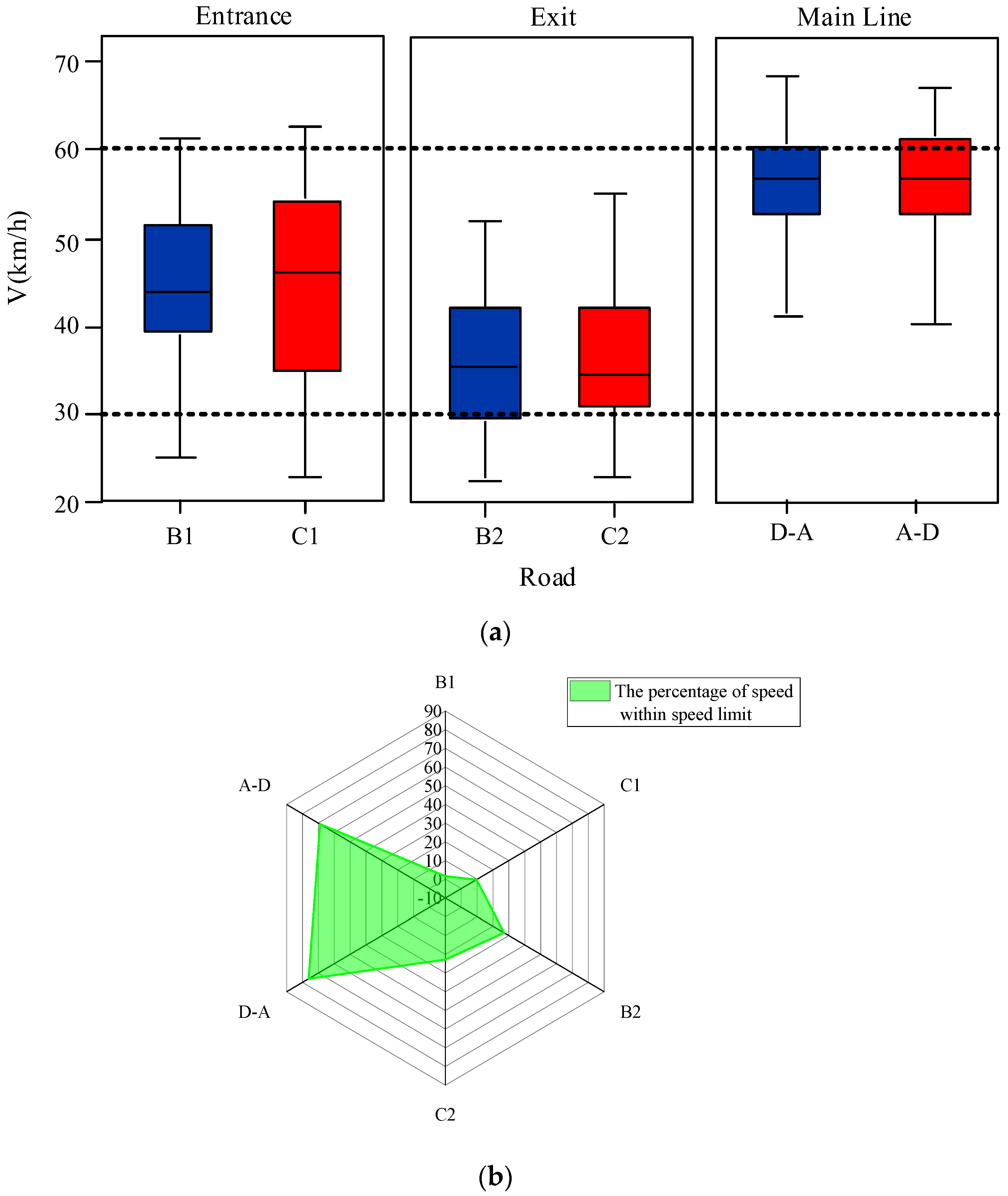
The driving speed of each route was determined, as shown in Figure 2. The speed of vehicles entering the ramp was slightly higher than that when leaving the ramp. Under the current speed limit of 30 km/h on the ramp, the drivers were speeding at the entrance and exit ramps. According to the statistics of the vehicles entering and exiting the ramp, the highest level of drivers observing the speed limit was only 26%. For the main line in the tunnel, when the speed limit was 60 km/h, although the degree of compliance improved compared with that of the ramp, there was also speeding, which accounts for 28–31%. Through the t-test of independent samples, it can be seen from the

Table 4. T-test significance results of independent samples.

Sig.	B1	C1	B2	C2	D–A	A–D
B1	-	0.000	0.053	0.000	0.000	0.000
C1	0.000	-	0.000	0.000	0.000	0.000
B2	0.053	0.000	-	0.027	0.000	0.000
C2	0.000	0.000	0.027	-	0.000	0.000
D-A	0.000	0.000	0.000	0.000	-	0.000
A-D	0.000	0.000	0.000	0.000	0.000	-

that the speed difference between different sections is significant, sig. less than 0.05. Except for the speed difference between B1 and B2, sig. is 0.053, slightly greater than 0.05, but controlled within the range of 0.1. It can also be considered that there are significant differences in speed values between all sections. Therefore, the speed limit can be optimized according to the driving habits of subjects and environmental adaptability.

4. Effective Model and Parameter Calculation

4.1. MEET Model of Urban Underwater Tunnel

Assuming that the road gradient is zero and the vehicle is in an unloaded state, the MEET basic model listed in the literature [18] is used to roughly estimate the CO₂ emission factor in an urban underwater tunnel, calculated using Formula (4).

$$e=(110+0.000375v^3+8702/v)$$

(4)

where e is the CO₂ emission factor in g/km and v is the velocity in km/h.

When considering the gradient and vehicle load, the gradient and vehicle load correction coefficients mentioned in the literature [17] were used. The gradient is set to 5% of the maximum value of the longitudinal slope, and the vehicle is fully loaded, calculated using Formulas (5) and (6).

$$GF=\exp ((0.0059v^2-0.0775v+11.936)\gamma )$$

(5)

$$LC=(0.27)x+1+0.0614\gamma x-0.0011{\gamma }^{3}x-0.00235vx-(\frac{1.33}{v})x$$

(6)

where GF is the gradient correction factor, LC is the vehicle load correction factor, γ is the road gradient (%), and x is the ratio of vehicle load to vehicle capacity.

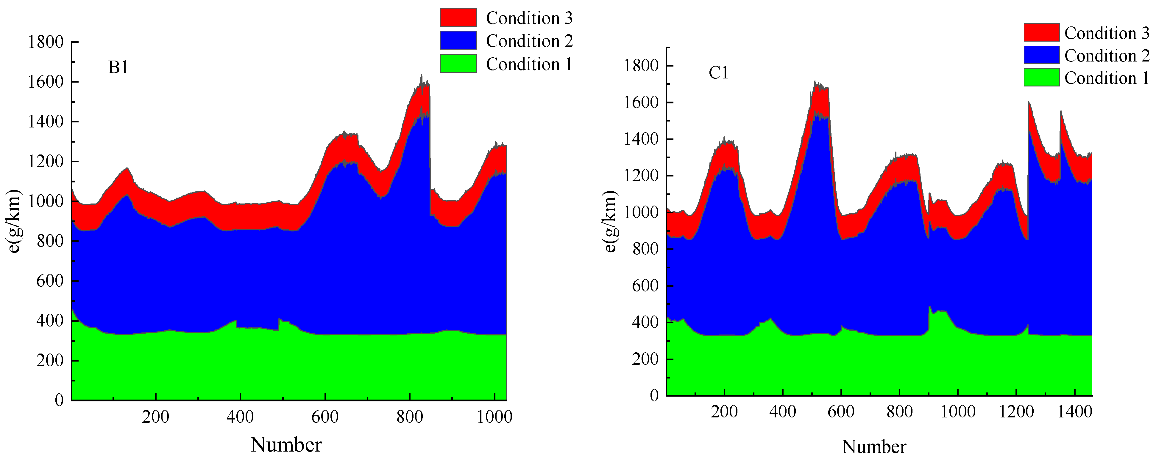
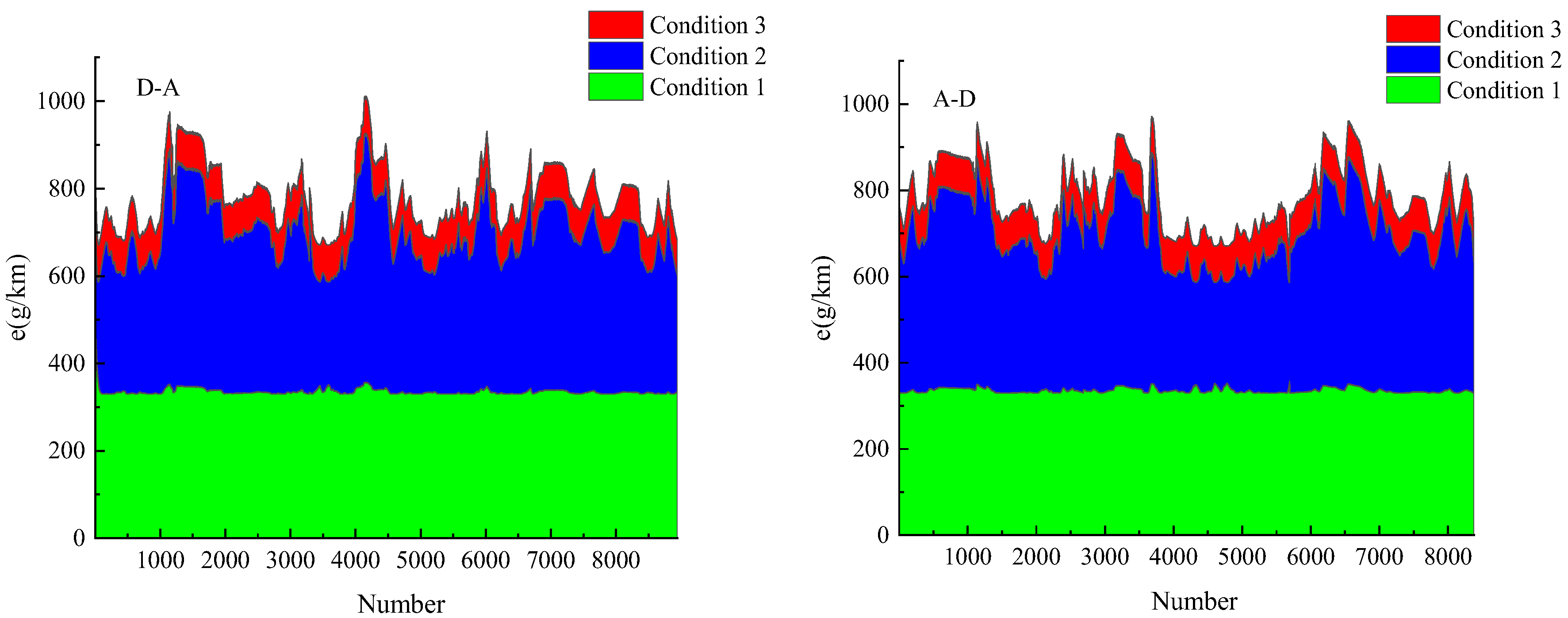
The CO₂ emissions factor of vehicles under different working conditions were considered according to the basic MEET model. Three working conditions were defined, and the CO₂ emissions factor under the corresponding conditions were calculated, as shown in Figure 3, Figure 4 and Figure 5. The average value of CO₂ emissions factor under different working conditions were calculated, as shown in

Table 5. CO₂ emissions factor under different working conditions. g/km.

-	Entrance of the Ramp		Exit of the Ramp		Main Line
	B1	C1	B2	C2	D–A	A–D
Condition 1	347.41	351.90	382.59	381.00	335.13	335.56
Condition 2	986.06	1059.07	894.39	891.51	780.82	787.42
Condition 3	1119.37	1197.12	1028.30	1024.99	699.94	706.44

.

Condition 1: The slope is 0 and the vehicle is empty.

When slope and vehicle load were not considered, the original CO₂ emissions factor in the urban underwater tunnel ramp calculated by the MEET model were evenly distributed in the range of 300–400 g/km. The average CO₂ emissions factor at ramp entrances B1 and C1 were 347.41 g/km and 351.90 g/km, respectively, and the average CO₂ emissions factor at ramp exits B2 and C2 were 382.59 g/km and 381.00 g/km, respectively. The main line area fluctuated less, at 330 g/km, and the average CO₂ emissions at D–A and A–D were 335.13 g/km and 335.56 g/km, respectively.

Condition 2: Maximum longitudinal slope and the vehicle is empty.

The road gradient is considered but the vehicle is empty, the maximum longitudinal slope of the ramp is 5%, and the maximum longitudinal slope of the main line is 2.8%. The no-load CO₂ emissions of urban underwater tunnel ramps calculated by the MEET model were distributed in the range of 800–1000 g/km. The ramp entrance CO₂ emissions factor fluctuated more than those at the exits. The average CO₂ emissions factor of ramp entrances B1 and C1 were 986.06 g/km and 1059.07 g/km, respectively, and the average CO₂ emissions factor of ramp exits B2 and C2 were 894.39 g/km and 891.51 g/km, respectively. The main line slightly varied at approximately 600 g/km, and the average CO₂ emissions factor at D–A and A–D were 780.82 g/km and 787.42 g/km, respectively.

Condition 3: Maximum longitudinal slope and the vehicle is fully loaded.

The slope is considered and the vehicle is fully loaded, the maximum longitudinal slope of the ramp is 5%, the maximum longitudinal slope of the mainline is 2.8%, and the full load is 1. The full-load CO₂ emissions factor of urban underwater tunnel ramps calculated by the MEET model were distributed at approximately 1000 g/km. The ramp entrance CO₂ emissions factor fluctuated more than those at the exit. The average CO₂ emissions factor of ramp entrances B1 and C1 were 1119.37 g/km and 1197.12 g/km, respectively, and the average CO₂ emissions factor of ramp exits B2 and C2 were 1028.30 g/km and 1024.99 g/km, respectively. The main line varied at approximately 700 g/km, and the average CO₂ emissions at D–A and A–D were 699.94 g/km and 706.44 g/km, respectively.

The average CO₂ emission factor of the main line is in a low state under any working condition. This is because the driving environment at the main line is simpler than entrance and exit, the vehicle is less affected by the outside world when driving, speed is high, and driving state is relatively stable.

When the slope and load are not considered, the average CO₂ emission factor at the exit is greater than that at the entrance, because the speed at the exit is lower than that at the entrance. Before entering the ramp entrance, there is an urban expressway, and the driver drives faster. There is still some space to reduce the speed to the specified speed limit.

Considering only the impact of slope, the average value of CO₂ emissions factor at the entrance is larger, indicating that slope have a greater impact on the entrance. The higher the speed, the greater the calculated slope correction factor.

At the same time, considering the influence of slope and load, the average value of CO₂ emissions factor at the entrance has a large fluctuation. That is, when entering the tunnel, it is a downhill section, and the driver’s operation is not stable enough. The average speed is high, but there is a sudden deceleration behavior.

The differences between B1 and C1, and B2 and C2, at the entrance and exit, calculated by the MEET model, were small; therefore, the two ramps can be combined to further consider potential differences in the directions of the entrance and exit.

4.2. COPERT Model of Urban Underwater Tunnel

This study combines the calculation model of the road section emission factor EFco₂ using the COPERT model. When calculating energy consumption, search the corresponding parameters, where α = 0.005, β = −0.253, γ = 20.952, δ = 0, ε = 0.001, θ = 0.091, τ = 3.51. The calculation formula of energy consumption factor (ECF, MJ/km) is shown in Equation (7). For vehicles using gasoline, r_FC:EC is 22.86, r_H:C is 1.86 [23,24]. CO₂ emissions factor was calculated using Equation (8).

$$ECF=\frac{0.005V^2-0.253V+20.952}{0.001V^2+0.091V+3.51}$$

(7)

$$E{F}_{C{O}_2}=72.45ECF$$

(8)

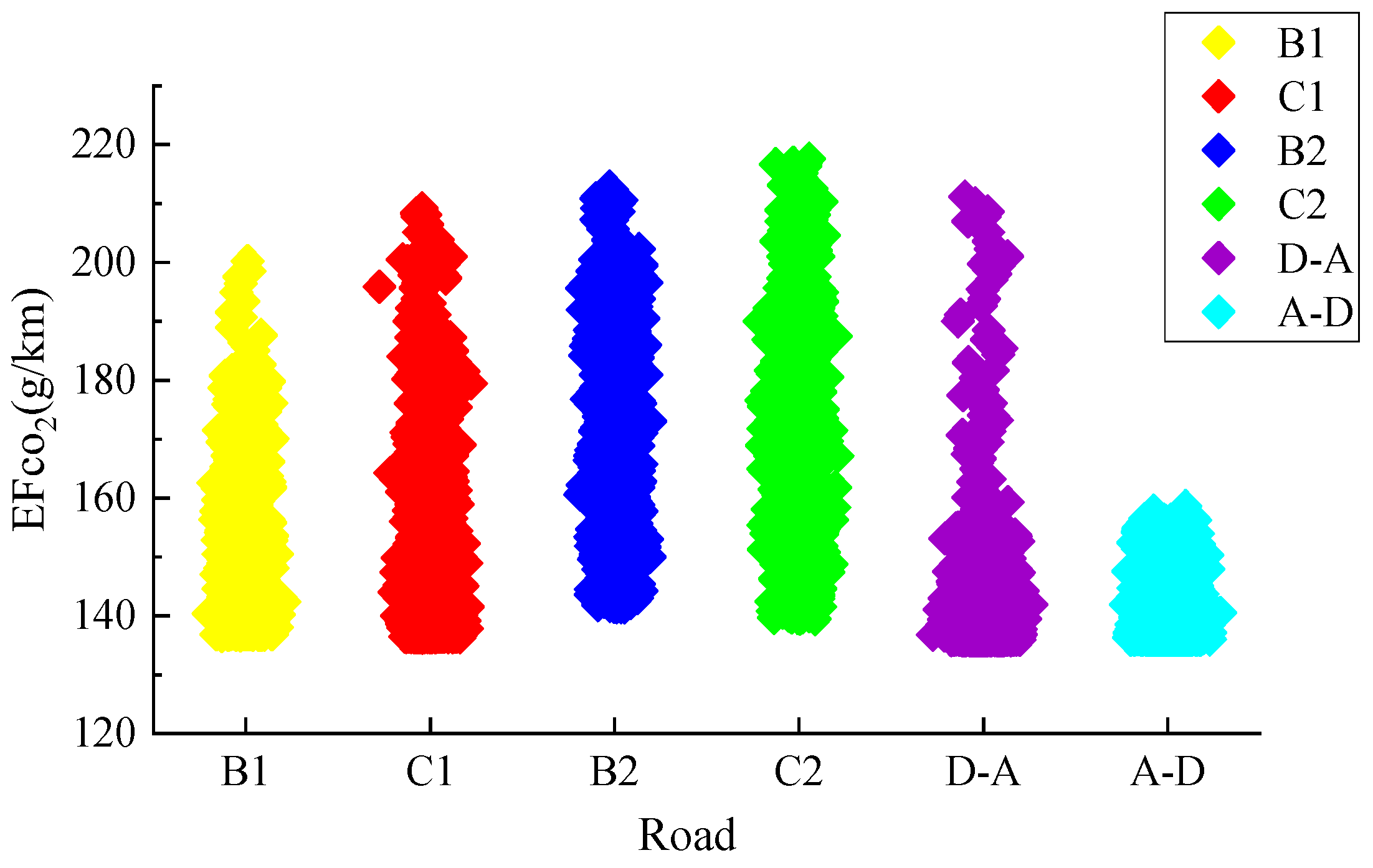
As shown in Figure 6, the emission factor EFco₂ calculated by the COPERT model at each ramp was relatively stable, distributed within the range of 140–200 g/km. The average CO₂ emissions factor of each ramp were 151.3 g/km (B1), 151.4 g/km (C1), 168.4 g/km (B2), and 167.8 g/km (C2). There is little difference in the distribution of CO₂ emissions factor between D and A of the tunnel’s main line and the ramp, also distributed within the range of 140–200 g/km, while A–D is more concentrated in the range of 140–160 g/km. The average CO₂ emissions factor of the main line was 139.8 g/km (D–A), 139.6 g/km (A–D). The differences between B1 and C1, and B2 and C2 in the entrances and exits calculated by the COPERT model were small, so the two ramps can also be combined to further consider differences in the directions of the entrances and exits.

4.3. Fit Speed–CO₂ Emissions Factor Model

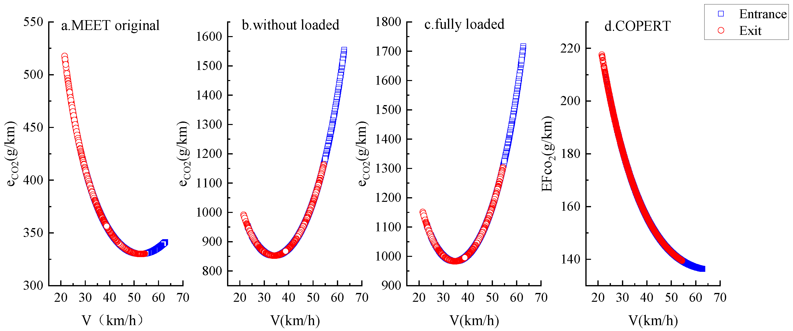
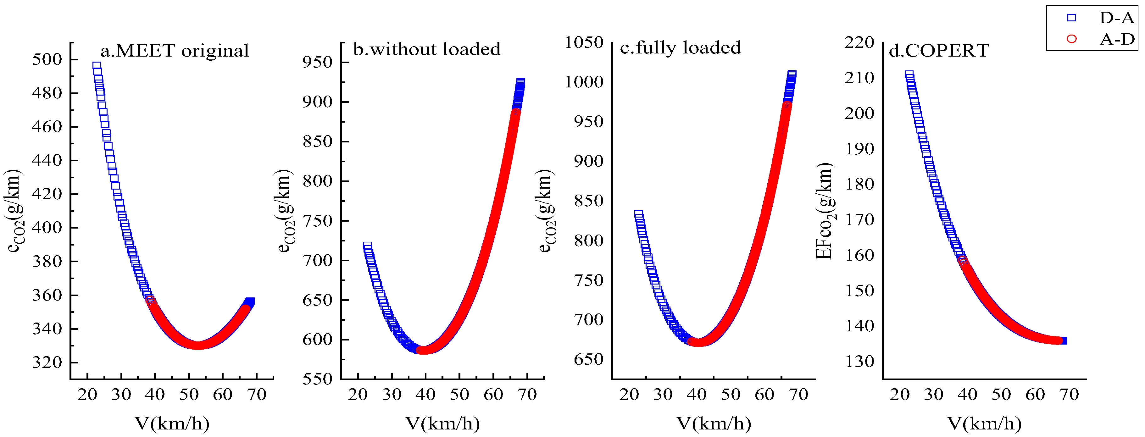
Based on the basic MEET and COPERT models, the relationship between speed and CO₂ emissions factor in urban underwater tunnels was explored. Figure 7a–c show the relationship between ramp entrance and exit speed and CO₂ emissions factor under the three working conditions of the MEET model. Figure 8a–c show the relationship between the speed in the main line of the tunnel and CO₂ emissions factor under the three working conditions of the MEET model. There is a valley point in the graph considering the slope and vehicle load, that is, the speed value corresponding to the lowest CO₂ emissions. Relevant data were extracted to obtain the speed value when CO₂ emissions factor were the lowest under each working condition. Those speeds in the entrance ramps were 52.76 km/h (Condition 1), 34.09 km/h (Condition 2), and 34.76 km/h (Condition 3). Speeds in the exit ramps were 52.76 km/h (Condition 1), 34.09 km/h (Condition 2), and 34.76 km/h (Condition 3). Speeds in the main line D–A were 52.73 km/h (Condition 1), 40.5 km/h (Condition 2), and 39.49 km/h (Condition 3). Speeds in the main line A–D were 52.73 km/h (Condition 1), 40.5 km/h (Condition 2), and 39.38 km/h (Condition 3).

The MEET model has limited factors of slope and load, although emerging scholars have added correction coefficients; therefore, it is complicated to obtain the vehicle load according to the actual conditions of the vehicles at the entrance and exit of the tunnel ramp and main line. It can be seen from the figure that when the load and slope are considered in the MEET model, as shown in Figure 7b,c and Figure 8b,c the change trend of the curve is opposite to Figure 7a,d and Figure 8a,d that is, the load correction factor and slope correction factor have a great impact on the results.

This is because relevant scholars have expanded the actual emission factor through the slope and load correction factor, and want to highlight the impact of slope and load on it. Therefore, the MEET model is more suitable for emission estimation that has clear indications for slope and load and does not require an input of the type of vehicle. The COPERT model emphasizes the impact of different vehicle models and fuel forms on CO₂ emissions. To estimate the CO₂ emissions of vehicle using gasoline in urban underwater tunnels in this study and to focus on the impact of a single factor (speed), the COPERT model is more suitable. Thus, based on the EFco₂ distribution obtained by the COPERT model, the relationship between speed and CO₂ emissions factor was further analyzed. Based on conclusions drawn from Figure 6, the difference in CO₂ emissions factor caused by different ramps is small. This begs further consideration of the entrance and exit directions, and whether the CO₂ emissions factor of vehicles are affected by the direction of the entrance and exit of the tunnel.

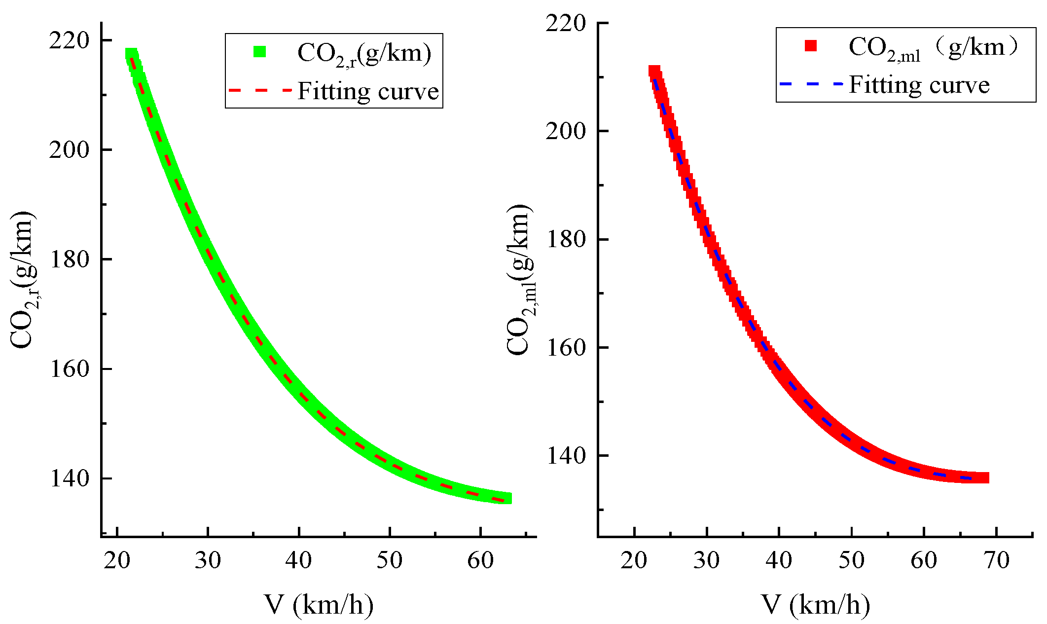
Figure 7d shows the relationship between speed and CO₂ emissions factor, in both directions of the ramp, calculated by the COPERT model, and Figure 8d shows the relationship between the mainline speed and CO₂ emissions factor. The speed at the tunnel is negatively correlated with the CO₂ emission factor; the maximum speed at the ramp appears on the exit ramp, and the maximum speed of the main line appears on the D–A line, but the two directions have a high degree of coincidence on the curve. Based on the speed and CO₂ emission factors obtained in these two directions, the relationship between the vehicle speed and CO₂ emissions in the urban underwater tunnel ramp and between the two directions of the main line was obtained. The fitting degree of the cubic polynomial is the best through fitting, so the urban underwater tunnel speed–CO₂ emissions factor model was set up as shown in Formula (9).

$$y=a{x}^3+b{x}^2+cx+d$$

(9)

From the analysis of the correlation between the entrance and exit speeds and CO₂ emissions factor, the difference between the two is small, and the correlation between speed and CO₂ emissions factor at the mainline is the same. Therefore, the overall speed–CO₂ emission factor model of the urban underwater tunnel ramp and the overall main line was obtained (Figure 9). The parameters of each model are listed in

Table 6. Speed–CO₂ emissions factor model parameters of tunnel vehicles.

—	a	b	c	d	R2
Entrance of the ramp	−0.0008	0.1604	−10.744	381.53	1
Exit of the ramp	−0.0011	0.1943	−12.035	397.42	1
D-A	−0.0007	0.1393	−9.848	369.69	0.99
A-D	−0.0005	0.1127	−8.3896	343.36	1
The whole of the ramp	−0.0009	0.1689	−11.1	386.3	1
The whole of the main lane	−0.0007	0.1387	−9.8068	368.77	0.99

.

The final urban underwater tunnel ramp-speed–CO₂ emissions factor model was obtained through Equation (10), and the mainline-speed–CO₂ emissions factor model was obtained through Equation (11).

$$C{O}_{2,r}=-0.0009V_r{}^3+0.1689V_r{}^2-11.1V_r+386.3$$

(10)

$$C{O}_{2,ml}=-0.0007V_{ml}{}^3+0.1387V_{ml}{}^2-9.8068V_{ml}+368.77$$

(11)

where CO_2,r is the CO₂ emissions factor at the ramp, g/km; CO_2,ml is the CO₂ emissions factor at the main line, g/km; V_r is the driving speed at the ramp, km/h; and V_ml is the driving speed at the main line, km/h.

5. Gasoline Consumption and Optimal Driving Speed Model

According to Wang et al. [28], sufficient combustion of CO₂ can effectively reduce harmful gases, such as CO. An optimal driving speed range makes the CO₂ emissions factor of the vehicle the highest; that is, fuel is the most abundant, and this speed range is defined as the optimal CO₂ emission driving speed range. A vehicle gasoline consumption model was proposed, as shown in Formula (12).

$$GC=-0.21637v+0.0013055v^2+0.24808IRI+13.36580$$

(12)

where GC is the gasoline consumption per 100 kilometers, L/100 km; V is the velocity in km/h; and IRI is the international flatness index (m/km), with an international reference value of 2.

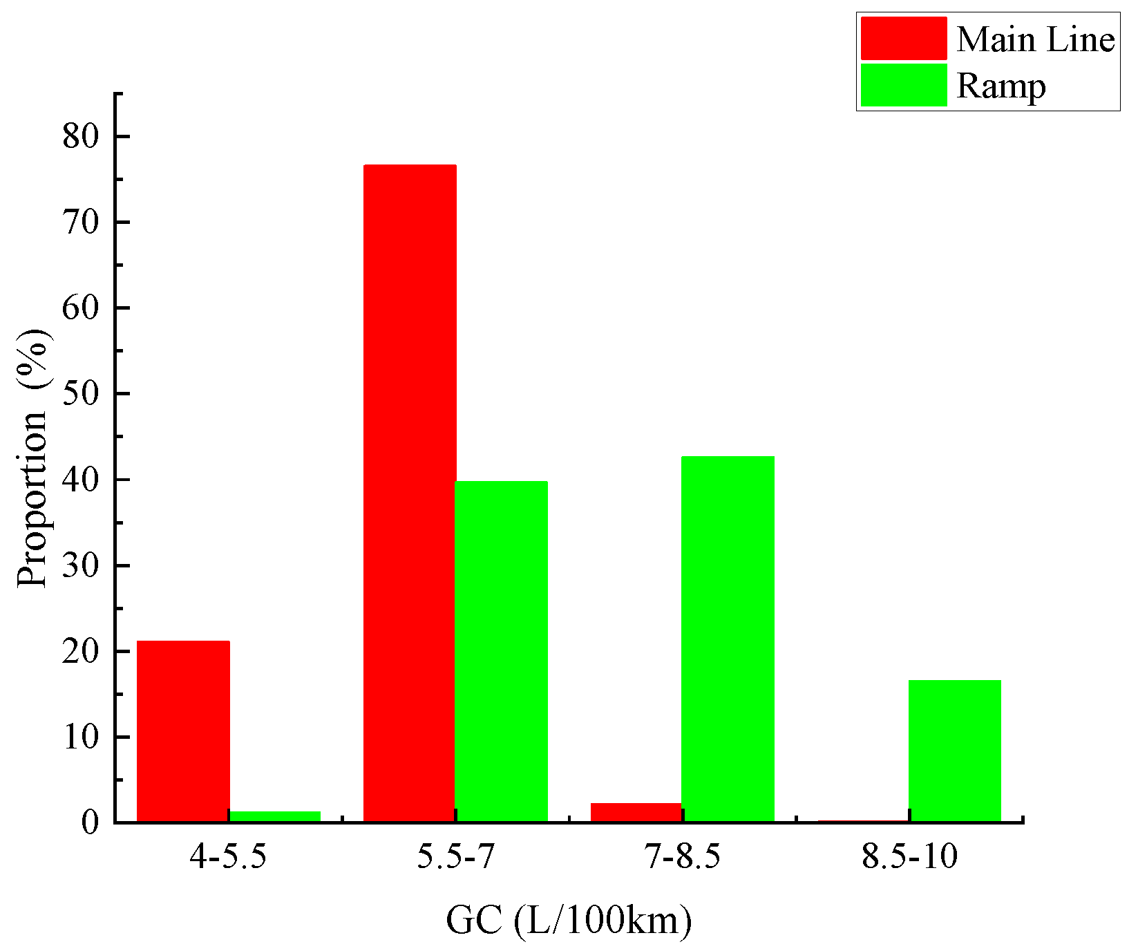
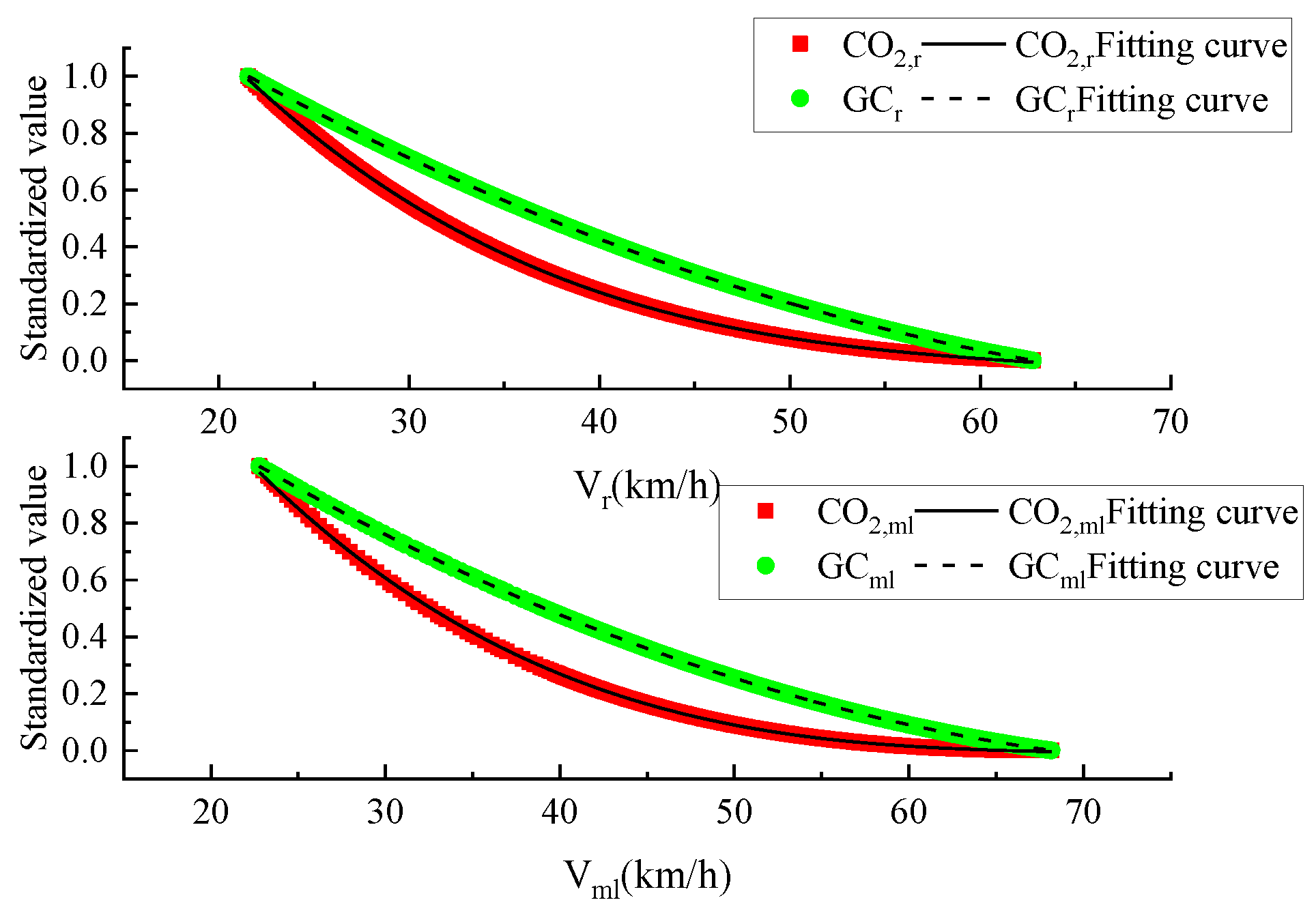
According to the calculated gasoline consumption value, draw the proportion diagram of gasoline consumption value in different intervals, as shown in Figure 10. The gasoline consumption distribution of vehicles at the ramp’s entrance and exit is mainly concentrated in the range of 7~8.5 L/100 km, and the main line is concentrated in the range of 5.5~7 L/100 km. Through MIN-MAX standardization, the gasoline consumption and CO₂ emissions factors at different speeds were normalized to determine the optimal driving speed range. The normalized speed–gasoline consumption model and speed–CO₂ emissions factor model are shown in Equation (13–16).

$$G{C}_r=0.0003v^2-0.0494v+1.9254$$

(13)

$$G{C}_{ml}=0.0003v^2-0.0488v+1.9594$$

(14)

$$C{O}_{2,r}=-1\cdot {10}^{-5}{v}^3+0.0021v^2-0.1367v+3.0774$$

(15)

$$C{O}_{2,ml}=-9\cdot {10}^{-6}{v}^3+0.0018v^2-0.1304v+3.0954$$

(16)

Figure 11 shows the relationship between the normalized gasoline consumption, CO₂ emissions factor, and speed. There is an intersection between the two. Through model fitting, the normalized fitting equation was calculated, the overall fitting model was restored, and the intersection of the fitting model was obtained. Since the CO₂ emissions factor is the highest within the optimal driving speed range, gasoline is the most abundant, that is, the region where CO_2,i is greater than GC. By solving the intersection of fitting Equations 13 and 15, it is obtained that the two curves of the ramp intersect at two places where v is 47 km/h and v is 21 km/h. Then, according to the limit of CO_{2, r} > GC_r, the optimal speed at the ramp is finally determined to be 47 km/h. Considering the safety factors and the overspeed characteristics of most drivers, the speed limit value of ramp section is 40 km/h after rounding.

Similarly, by solving the intersection of the fitting Equations 14 and 16, it is obtained that the intersection v of the two curves of the main line segment is 21 km/h. According to the limit of CO_{2, ml} > GC_ml and the actual driving speed of the main line segment, the intersection with v of 21 km/h is discarded. According to the linear trend, when v is greater than 81 km/h (the valley value of GC_ml curve), the two curves of CO_{2, ml} and GC_ml gradually move away. Therefore, the best speed range should be less than 81 km/h, and finally determine to maintain the existing limited speed of 60 km/h at the main line. It can provide a basis for resetting the speed limit value of the urban underwater tunnel, so that vehicle travel speed is more environmentally friendly.

6. Conclusions

Through the comparative analysis of MEET and COPERT models, considering that COPERT model emphasizes the impact of different vehicle types and different fuel forms on CO₂ emissions factor, it is more suitable for CO₂ emissions factor estimation of small gasoline vehicles in urban underwater tunnels, which focuses on the impact of a single factor of speed in this paper. Therefore, COPERT is selected as the basic model for calculating the emission of cars at the urban underwater tunnel, and the V_r–CO_2,r and V_ml–CO_2,ml models of the urban underwater tunnel are constructed through practical examples. The main conclusions are as follows.

(1)

Under the influence of the existing speed limit conditions, more than 70% of drivers on the ramp did not obey the speed limit rules, as well as 30% of drivers on the main lines;

(2)

Without considering the influence of road slope and vehicle load, there is a negative correlation between speed and CO₂ emissions factor in MEET model. When affected by slope and load, these positive influence factors change the correlation of the original model, expand the size of CO₂ emissions factor, and make the calculated values deviate from the actual size. It is only applicable to the research of parameter trend analysis, not applicable to further calculation research based on CO₂ emissions factor;

(3)

COPERT model estimates CO₂ emissions factor by calculating the gasoline consumption coefficient. When only considering the influence of gasoline consumption and speed parameters, the CO₂ emissions factor is negatively correlated with speed. There are fewer variables in the model, and the parameters are more controllable and more in line with the actual situation;

(4)

The gasoline consumption distribution of vehicles at the ramp entrance and exit is mainly concentrated in the range of 7~8.5 L/100 km, while the main line is concentrated in the range of 5.5~7 L/100 km. By normalizing the gasoline consumption and CO₂ emissions factor, the standardized fitting models at the ramp and the main line segment are obtained respectively;

(5)

Due to the highest proportion of CO₂ emissions factor and the most sufficient fuel in the optimal driving speed range, the region of CO_{2, i} > GC_i in the standardized fitting model is selected to finally determine the limited speed applicable to the current urban underwater tunnel, with a ramp of 40 km/h, main line is 60 km/h.

This research combines the existing basic model framework with actual driving data of a real vehicle test to obtain the CO₂ emissions factor model of an urban underwater tunnel. However, the relevant parameters of the original basic model are retained in the model framework. For example, the calculation parameters of fuel consumption, the car-bon-hydrogen ratio of different fuels, and the relationship between the fuel consumption coefficient and energy consumption. The test considered only the CO₂ emissions factor from gasoline-powered vehicles. However, as there are currently vehicles running on alternative energy sources, their CO₂ emissions during driving can be the focus of future research.

References

1. Vicente, F.; Marina, K.; Marilena, M.; Leonidas, N.; Stefan, H.; Panagiota, D. Road vehicle emission factors development: A review. Atmos. Environ. 2013, 70, 84–97. [Google Scholar] [CrossRef]
2. Wang, X.; Liu, M.; Ci, Y.; Yang, Y. Effectiveness of driver’s bounded rationality and speed guidance on fuel-saving and emissions-reducing at a signalized intersection. J. Clean. Prod. 2021, 325, 129343. [Google Scholar] [CrossRef]
3. Hyung-Wook, C.; Christopher Frey, H. Estimating diesel vehicle emission factors at constant and high speeds for short road segments. Transp. Res. Rec. 2010, 2158, 19–27. [Google Scholar] [CrossRef]
4. Zhang, J.; Yu, L.; Guo, J.; Cheng, Y.; He, W.; Song, G. Optimized adjustment of speed resolution and time alignment data for improving emissions estimations. Transp. Res. Rec. 2016, 2570, 77–86. [Google Scholar] [CrossRef]
5. Wang, Y.; Xing, Z.; Zhang, H.; Wang, Y.; Du, K. On-road mileage-based emission factors of gaseous pollutants from bi-fuel taxi fleets in China: The influence of fuel type, vehicle speed, and accumulated mileage. Sci. Total Environ. 2022, 819, 151999. [Google Scholar] [CrossRef]
6. Chandrashekar, C.; Chatterjee, P.; Pawar, D. Estimation of CO2 and CO emissions from auto-rickshaws in Indian heterogeneous traffic. Transp. Res. Part D: Transp. Environ. 2022, 104, 103202. [Google Scholar] [CrossRef]
7. Vanatta, M.; Rathod, B.; Calzavara, J.; Courtright, T.; Sims, T.; Saint-Sernin, É.; Clack, H.; Jagger, P.; Craig, M. Emissions impacts of electrifying motorcycle taxis in Kampala, Uganda. Transp. Res. Part D: Transp. Environ. 2022, 104, 103193. [Google Scholar] [CrossRef]
8. Ashik, F.; Rahman, M.H.; Kamruzzaman, M. Investigating the impacts of transit-oriented development on transport-related CO2 emissions. Transp. Res. Part D Transp. Environ. 2020, 105, 103227. [Google Scholar] [CrossRef]
9. Jiao, F.; Du, Z.; Chen, G.; Zheng, H.; Tang, Z.; Wang, S. Entrance zone length of extra-long undersea tunnels based on vision adaptation. Tunn. Undergr. Space Technol. 2021, 113, 103970. [Google Scholar] [CrossRef]
10. Jiao, F.; Du, Z.; Yiik, D.; He, S.; Xu, F.; Zheng, H. Self-explaining performance of visual guiding facilities in urban road tunnels based on speed perception. Tunn. Undergr. Space Technol. 2022, 122, 104371. [Google Scholar] [CrossRef]
11. Yang, Y.; Du, Z.; Jiao, F.; Pan, F. Analysis of EEG Characteristics of drivers and driving safety in undersea tunnel. Int. J. Environ. Res. Public Health 2021, 18, 9810. [Google Scholar] [CrossRef] [PubMed]
12. Fu, L.; He, K.; He, D.; Tang, Z.; Hao, J. A study on models of MOBILE source emission factors. Acta Sci. Circumstantiae 1997, 17, 89–94. [Google Scholar] [CrossRef]
13. Shan, X.; Liu, H.; Zhang, X.; Chen, X.; Ye, J. Localization of light-duty vehicle emission factor estimation based on MOVES. J. Tongji Univ. (Nat. Sci.) 2021, 49, 1135–1143. [Google Scholar] [CrossRef]
14. Arne, H. Comparing emission estimation models for rail freight transportation. Transp. Res. Part D Transp. Environ. 2020, 86, 102468. [Google Scholar] [CrossRef]
15. Duan, Z. Research on the Peak Mechanism and Peak Comprehensive Judgment System of Carbon Emissions under the Evolution of Social Economic System. Ph.D. Thesis, Jilin University, Changchun, China, 2021. [Google Scholar] [CrossRef]
16. Hickman, A. Methodology for Calculating Transport Emissions and Energy Consumption; European Commission: Luxembourg, 1999. [Google Scholar]
17. Mansoureh, N.; Mahdi, A. Measurement, evaluation and minimization of CO2, NOx, and CO emissions in the open time dependent vehicle routing problem. Measurement 2016, 90, 443–452. [Google Scholar]
18. Liu, C.; Shen, L.; Shen, H.; Lv, X.; Zhai, Y. Research on low-carbon time-dependent vehicle routing problem with traffic congestion avoidance approaches. Control. Decis. 2020, 35, 2486–2496. [Google Scholar] [CrossRef]
19. Zhang, Z.; Song, G.; Zhang, L.; Zhai, Z.; He, W.; Yu, L. How do errors occur when developing speed correction factors for emission modeling. Transp. Res. Part D Transp. Environ. 2021, 101, 103094. [Google Scholar] [CrossRef]
20. Zhai, Z.; Xu, J.; Song, G.; Hatzopoulou, M. Comparative analysis of drive-cycles, speed limit violations, and emissions in two cities: Toronto and Beijing. Sci. Total Environ. 2022, 11, 152323. [Google Scholar] [CrossRef]
21. Davison, J.; Bernard, Y.; Borken-Kleefeld, J.; Farren, N.J.; Hausberger, S.; Sjödin, Å.; Tate, J.E.; Vaughan, A.R.; Carslaw, D.C. Distance-based emission factors from vehicle emission remote sensing measurements. Sci. Total Environ. 2020, 739, 139688. [Google Scholar] [CrossRef]
22. Xu, L.; Wang, L.; Liu, Y.; Song, G.; Li, C.; Zhai, Z. Calculation model of bus energy consumption and CO2 emission based on multi-source data. J. Transp. Syst. Eng. Inf. Technol. 2020, 20, 174–181. [Google Scholar] [CrossRef]
23. He, Y.M. Estimating and Analyzing Spatiotemporal Patterns of Vehicle CO2 Emissions in Urban Road Based on GPS Data. Master’s Thesis, Chang’an University, Xian, China, 2020. [Google Scholar] [CrossRef]
24. EMEP/EEA. Air Pollutant Emission Inventory Guidebook 2019; Publications Office of the European Union: Luxembourg, 2021; Available online: https://www.eea.europa.eu/publications/emep-eea-guidebook-2019 (accessed on 10 June 2022).
25. Ali, M.; Kamal, M.; Tahir, A.; Atif, S. Fuel consumption monitoring through COPERT model—A case study for urban sustainability. Sustainability 2021, 13, 11614. [Google Scholar] [CrossRef]
26. Ekström, M.; Sjödin, Å.; Andreasson, K. Evaluation of the COPERT III emission model with on-road optical remote sensing measurements. Atmos. Environ. 2004, 38, 6631–6641. [Google Scholar] [CrossRef]
27. Xie, S.; Song, X.; Shen, X. Calculating vehicular emission factors with COPERTIII mode in China. Environ. Sci. 2006, 27, 3415–3419. [Google Scholar] [CrossRef]
28. Wang, L.; Ji, H.; Wang, H. Research on driving speed range based on optimum carbon emission and fuel consumption optimization. Transp. Energy Conserv. Environ. Prot. 2020, 16, 4–8. [Google Scholar]
Figure 1. Topographic map of entrance and exit.
Sustainability 14 09592 g001
Figure 2. Driving speed. (a) Velocity distribution. (b) Proportion within speed limit value of each road section.
Sustainability 14 09592 g002
Figure 3. Entrance to the ramp.
Sustainability 14 09592 g003
Figure 4. Exit of the ramp.
Sustainability 14 09592 g004
Figure 5. The main line of the tunnel.
Sustainability 14 09592 g005
Figure 6. Distribution of CO2 emissions factor.
Sustainability 14 09592 g006
Figure 7. Speed–CO2 emissions factor model for each mode of the ramp.
Sustainability 14 09592 g007
Figure 8. Speed–CO2 emissions factor model for each mode of the main line.
Sustainability 14 09592 g008
Figure 9. Speed–CO2 emissions factor model of tunnel vehicles.
Sustainability 14 09592 g009
Figure 10. Proportion of gasoline consumption values in different intervals.
Sustainability 14 09592 g010
Figure 11. Normalized model.
Sustainability 14 09592 g011