A Study on the Optimal Flexible Job-Shop Scheduling with Sequence-Dependent Setup Time Based on a Hybrid Algorithm of Improved Quantum Cat Swarm Optimization

Abstract

Multi-item and small-lot-size production modes lead to frequent setup, which involves significant setup times and has a substantial impact on productivity. In this study, we investigated the optimal flexible job-shop scheduling problem with a sequence-dependent setup time. We built a mathematical model with the optimal objective of minimization of the maximum completion time (makespan). Considering the process sequence, which is influenced by setup time, processing time, and machine load limitations, first, processing machinery is chosen based on machine load and processing time, and then processing tasks are scheduled based on setup time and processing time. An improved quantum cat swarm optimization (QCSO) algorithm is proposed to solve the problem, a quantum coding method is introduced, the quantum bit (Q-bit) and cat swarm algorithm (CSO) are combined, and the cats are iteratively updated by quantum rotation angle position; then, the dynamic mixture ratio (MR) value is selected according to the number of algorithm iterations. The use of this method expands our understanding of space and increases operation efficiency and speed. Finally, the improved QCSO algorithm and parallel genetic algorithm (PGA) are compared through simulation experiments. The results show that the improved QCSO algorithm has better results, and the robustness of the algorithm is improved.

1. Introduction

Since 1990, the flexible job-shop scheduling problem (FJSP) has attracted attention due to its wide application and high complexity. In the last decades, fruitful results have been reported concerning the FJSP. To narrow the gap between the problem and practical manufacturing, the general FJSP was extended by considering some additional practical factors. In those extended FJSP problems, setup time is a commonly considered factor. In many real-life manufacturing systems, the setup operations, such as cleaning up or changing tools, are not only often required between jobs but also strongly depend on the immediately preceding process on the same machine. This motivates researchers to study the FJSP with sequence-dependent setup time (SDST). It is well known that the general FJSP has been proven to be an NP-hard problem. As an extended problem, SDST is obviously more complex than the general FJSP. Therefore, efficient methods are needed to acquire satisfactory solutions that are of high quality in a reasonable computational time. Considering that exact methods are too intractable to solve the problem, heuristic algorithms have received extensive attention from scholars. A summary of research optimization algorithms on FJSP-SDST is presented in

Table 1. Summary of research optimization algorithms on FJSP-SDST.

Literature	Objective Function	Algorithms
Mousakhani [2]	Minimize total tardiness	Iterated local search
Shen et al. [3]	Minimize makespan	Tabu search with specific neighborhood search function
Bagheri and Zandieh [4]	Minimize makespan and mean tardiness	Variable neighborhood search
Abdelmaguid [5]	Minimize makespan	Tabu search with specific neighborhood functions
Naderi et al. [6]	Minimize makespan	Genetic algorithm
Li and Lei [7]	Minimize makespan, total tardiness, and total energy consumption	Imperialist competitive algorithm with feedback
Defersha and Chen [8]	Minimize makespan	Parallel genetic algorithm
Azzouz et al. [9]	Minimize makespan and bi-criteria objective function	Hybrid genetic algorithm and variable neighborhood search
Wang and Zhu [10]	Minimize makespan	Hybrid genetic algorithm and tabu search
Li et al. [11]	Minimize makespan and total setup costs	Elitist nondominated sorting hybrid algorithm
Azzouz et al. [12]	Minimize makespan	Hybrid genetic algorithm and iterated local search
Azzouz et al. [13]	Minimize makespan	Adaptive genetic algorithm
Abderrabi et al. [14]	Minimize total flow time	Genetic algorithm and iterated local search
Parjapati and Ajai [15]	Minimize makespan	Genetic algorithm
Sadrzadeh [16]	Minimize makespan and mean tardiness	Artificial immune system and particle swarm optimization
Tayebi Araghi et al. [17]	Minimize makespan	Genetic variable neighborhood search with affinity function
Sun et al. [18]	Minimize makespan, total workload, workload of critical machine, and penalties of earliness/tardiness	Hybrid many-objective evolutionary algorithm
Li et al. [19]	Minimize energy consumption and makespan	Improved Jaya algorithm
Müller et al. [20]	Minimize makespan	Decision trees and deep neural networks
Wei et al. [21]	Minimize the makespan and total energy consumption	Energy-aware estimation model
Li et al. [22]	Minimize the makespan and the total workload	Hybrid self-adaptive multi-objective evolutionary algorithm
Türkyılmaz et al. [23]	Minimize makespan	Hybrid Genetic Algorithm-hypervolume contribution measure
Jiang et al. [24]	Handle the issues of low production efficiency, high energy consumption and processing cost	A novel improved crossover artificial bee colony algorithm

. With regard to the previous work, various heuristic algorithms have been adopted, but no heuristic can perform best for all types of SDST problems or all instances of the same problem, which is in accordance with the “no free lunch” theorem [1]. This is also the main motivation behind presenting a fresh heuristic algorithm for the considered SDST problem.

Exploration and exploitation are treated as the most important features of heuristic algorithms. The trade-off between the two features is crucial to the computational performance. However, for many famous heuristics, some algorithms have a better global search ability, such as particle swarm optimization (PSO), ant colony optimization (ACO), the genetic algorithm (GA), and the whale optimization algorithm (WOA) [25], while others have a better local search ability, such as simulated annealing (SA), variable neighborhood search (VNS), the crow search algorithm (CSA) [26], and tabu search (TS). Compared to the mentioned algorithms, cat swarm optimization (CSO), a novel swarm intelligence algorithm proposed by Chu et al. [27], is inspired by the behavioral modes of cats in nature, specifically their seeking mode and tracing mode, corresponding to global search and local search in the algorithm. The main advantage of the CSO algorithm is that the local and global search can be performed simultaneously during the evolutionary process. This feature provides the chance to find a balance between exploration and exploitation by elaborately designing the algorithm. Since it was proposed, CSO has been successfully applied to various optimization problems [28,29,30,31,32,33,34,35,36,37]. However, to the best of our knowledge, it is seldom adopted for SDST. Therefore, the aim of this paper is to apply CSO to the FJSP-SDST. To enhance the search ability, the quantum computing principle is incorporated with the conventional CSO to form quantum cat swarm optimization (QCSO). In QCSO, some improvements are made, as follows: (1) Quantum encoding is employed to enhance the search ergodicity of the algorithm. (2) The individual positions of cats are updated by adjusting the quantum rotation angle to improve the search efficiency and speed of the algorithm. (3) A dynamic adjustment strategy for the mixture ratio of the two search modes (seeking and tracing) is adopted to maintain the balance between exploration and exploitation. Extensive experimental results demonstrate that the proposed QCSO is effective in solving the considered problem.

The remainder of this paper is structured as follows: Section 2 describes the presented problem. Section 3 presents the proposed QCSO algorithm. Section 4 describes the extensive experiments and analyzes the computational results. Section 5 provides the conclusions and future work.

2. Problem Description and Formulation

2.1. Problem Assumption

In a workshop, n jobs {J₁, J₂, ⋯, J_n} need to be processed by m machines {M₁, M₂, ⋯, M_m}. Each job contains O_i operations and its own processing route. O_ij represents the jth operation of the ith job. Each operation O_ij can be processed on any machine selected from a compatible machine set. The processing time of each operation is determined by the processing capacity of the assigned machine. The setup time of each machine depends on the two consecutive operations on it. In this study, we chose an eligible machine for each operation, then sequenced the operations on each machine in order to minimize the makespan, i.e., $\min C=\min \left\{\max C_k|1\le k\le m\right\}$, where C_k represents the completion time of the last job on machine k. For this problem, the following assumptions help to simplify the problem:

(1)

Machines and jobs are available at time zero.

(2)

There exist precedence constraints among different operations of the same job, i.e., each operation can only be processed after its predecessor is completed.

(3)

There are no precedence constraints among different jobs, i.e., jobs are independent of each other.

(4)

Preemption is not allowed, i.e., the processing of each operation must not be interrupted once it starts.

(5)

Each machine can only process one operation at a given time.

(6)

Job transportation and machine breakdown are not considered.

2.2. Description of Parameters and Variables

Some necessary parameters and variables are shown in

Table 2. Some necessary parameters and variables.

Index	Explanation
J	Job set
O	Operation set
M	Machine set
$C_{\max }$	Final completion time (makespan)
$C_k$	Completion time of machine k
co, j,k	Completion time of operation o of job j on machine k
po, j,k	Processing time of operation o of job j on machine k
so, j,k,o’,j’	Setup time of two adjacent operations arranged on the same machine
sto, j, k	Start time of operation o of job j on machine k
Rm	Maximum number of processing tasks on machine m
r	Position index of processing tasks on each machine, r = 1, 2, ⋯, Rm
L	A large positive number
cr,k	Completion time of task r on machine k
xo,j,k	xo,j,k = 1 if operation o of job j is processed on machine k, otherwise xo, j,k = 0
yr,k,o,j	yr,k,o,j = 1 if the task on position r of machine k is just operation o of job j, otherwise yr,k,o,j = 0

.

2.3. Problem Formulation

$$\min C_{\max }=\min \{\max C_k\left|1\le k\right.\le m\}$$

(1)

$$c_{r,k}\ge c_{o,j,k}+L\times y_{r,k,o,j}-L$$

(2)

$$c_{r,k}-p_{o,j,k}-s_{o,j,k,o^{\prime },j^{\prime }}-L\times (y_{r,k,o,j}+y_{r-1,k,o^{\prime },j^{\prime }}+2L\ge c_{r-1,k} \{(r>1)\wedge (o,j)\ne (o^{\prime },j^{\prime })\}$$

(3)

$$y_{r,k,o,j}\le x_{o,j,k}$$

(4)

$${\displaystyle \sum _{k=1}^m{\displaystyle \sum _{r=1}^{R_m}{y}_{r,k,o,j}}}=1$$

(5)

$$y_{r^{\prime },k,o^{\prime },j}\le y_{r,k,o,j},\{(o^{\prime }>o)\wedge (r^{\prime }<r)\}$$

(6)

$$y_{r^{\prime },k,o^{\prime },j}\le 1-y_{r,k,o,j},\{(o^{\prime }<o)\wedge (r^{\prime }>r)\}$$

(7)

Equation (1) gives the objective function aiming to minimize the makespan. Constraints (2) and (3) show that the operation o of job j is just the processing task on position r of machine k. Constraints (4) and (5) indicate that any operation must be assigned to only one machine. Constraint (6) shows that if operation o of job j is arranged on position r of machine k, then any successive operation o’ of job j cannot be arranged on any earlier run r’ of machine k for processing. Constraint Equation (7) is a symmetric constraint of Constraint Equation (6); in other words, it ensures that the precedence activity of the job has been processed.

3. Implementation of Proposed QCSO

3.1. Encoding Approach

To implement QCSO, the first task is to design an appropriate encoding approach. Here, the probability amplitude is used to represent the current position of each individual cat. This paper maintains a population of Q-bit individuals, $Q(t)=\{q_1^t,q_2^t,\cdots ,q_N^t\}$ at generation t, where N is the size of the population and $q_i^t$ is a Q-bit individual, defined as:

$$q_i^t=\left(\left.\begin{array}{c}{\alpha }_{i1}^t\\ {\beta }_{i1}^t\end{array}\right|\left.\begin{array}{c}{\alpha }_{i2}^t\\ {\beta }_{i2}^t\end{array}\right|\begin{array}{c}\cdot \cdot \cdot \\ \cdot \cdot \cdot \end{array}\left|\begin{array}{c}{\alpha }_{in\times m}^t\\ {\beta }_{in\times m}^t\end{array}\right.\right), j=1,2,\dots ,N$$

(8)

where ${\left({\alpha }_{ij}^t,{\beta }_{ij}^t\right)}^T$, (i = 1, 2, …, n × m) is a Q-bit that should satisfy the normalization condition, ${\left|{\alpha }_{ij}^t\right|}^2+{\left|{\beta }_{ij}^t\right|}^2=1$. ${\left|{\alpha }_{ij}^t\right|}^2$ gives the probability that the Q-bit will be found in the 0 state and ${\left|{\beta }_{ij}^t\right|}^2$ gives the probability that the Q-bit will be found in the 1 state. According to what is observed, Q(t) can collapse to binary string P(t) composed by 0 and 1. A random number r is generated from the range [0, 1]; if r > ${\left|{\beta }_{ij}^t\right|}^2$, the bit of the binary string is set to 1. Thus, a binary string of length L is formed from the Q-bit individual. Meanwhile, every L binary string is converted to a decimal string in the range of 0 to n. Then, a decimal string of length n × o is formed. The decimal string is sorted from small to large to get the location, and its procedures are encoded.

For the FJSP with O procedures, n jobs, and m machines, the individual length of a quantum bit is defined as $L=([{\log }_2^n]+1)\times n\times o$, where [x] represents an integer that is not more than x.

3.2. Decoding Mechanism

This paper investigates the FJSP-SDST with the purpose of facilitating high achievement for all performance indices, such as the makespan of jobs, under the conditions of satisfying the process constraints, ensuring that the precedence activities of the job are completed, and minimizing the setup time of the work procedure of the same machine. The quantum individual is a linear superposition state of the solution through the probability amplitude, so the solution of the linear superposition state should be translated into a decimal solution through the decoding mechanism [38]. Because $[{\log }_2^n]+1\ge {\log }_2^n$, every $[{\log }_2^n]+1$ binary string should be converted to a decimal number, and finally a decimal string of length m × n is formed. The decimal string is sorted in order from small to large to make sure that the relative position of each number is unchanged. The smallest numbers of m represent the first job, while the next smallest numbers represent the second job. In this way, we can get the decimal string based on the working procedure code.

Step 1: Set P(t) as a Q-bit individual:

$$P(t)=\left[\left.\begin{array}{c}{\alpha }_1^{\prime }\\ {\beta }_1^{\prime }\end{array}\right|\left.\begin{array}{c}{\alpha }_2^{\prime }\\ {\beta }_2^{\prime }\end{array}\right|\begin{array}{c}\cdot \cdot \cdot \\ \cdot \cdot \cdot \end{array}\left|\begin{array}{c}{\alpha }_n^{\prime }\\ {\beta }_n^{\prime }\end{array}\right.\right]$$

(9)

where t represents the generation of the qubit, and in order to increase the chance that each solution will be searched, ${\alpha }_i^0$ and ${\beta }_i^0(i=1,2,\cdots n)$ are initialized with $\frac{\sqrt{2}}{2}$.

Step 2: Generate a random number r from the range [0, 1]; if ${\left|{\alpha }_i^{\prime }\right|}^2>r^2$, let x_i(t) = 1, else let x_i(t) = 0 (i = 1, 2, …, n). For every P(t), we can get a binary $X\left(t\right)=\left(x_1^{\prime },x_2^{\prime },\cdots ,x_n^{\prime }\right)$ of length n.

Step 3: In X(t), convert each $[{\log }_2^n]+1$ binary string to a decimal string, to form a decimal string $D(t)=(d_1^{\prime },d_2^{\prime },\cdots ,d_{m\times n}^{\prime })$ of length m × n.

Step 4: Let the numbers in D(t) be ordered from small to large; the smallest numbers of m represent the first job, the next smallest numbers represent the second job, and so on. The relative position of each number in D(t) is kept constant during the process. Thus, we can get a permutation W(t), by which each n job serial number is repeated m times. The number i that appears in W(t) for j times will represent operation j of job i. If there are two or more of the same numbers in D(t), then the smaller serial number represents the job that has the smaller process number.

The data processing of the 4 × 3 scale problem is shown in

Table 3. Data processing of a 4 × 3 scale problem.

Job	Number of Machine
1	1	2	3
2	3	1	2
3	1	3	2
4	2	3	1

, and the specific decoding process is as follows:

For example, in the 4 × 3 scale JSP, which includes 4 jobs and 3 machines, P(t) is a 36-bit qubit chromosome. Observing P(t), if we get the 36 binary string X(t) = {0, 1, 1, 1, 0, 1, 1, 0, 1, 1, 0, 0, 1, 1, 0, 0, 0, 0, 1, 1, 1, 0, 0, 0, 0, 1, 0, 0, 1, 0, 0, 0, 1, 1, 1, 0}, then D(t) = (2, 2, 2, 1, 2, 0, 3, 0, 1, 1, 1, 2). So positions 4, 6, and 8 comprise job 1; positions 9, 10, and 11 comprise job 2; positions 1, 2, and 3 comprise job 3; and position 5, 7, and 12 comprise job 4, and W(t) = (3, 3, 3, 1, 4, 1, 4, 1, 2, 2, 2, 4). The number 3 in position 1 represents the first operation of job 3, the number 1 in position 6 represents the second operation of job 1, and the number 4 in position 12 represents the third operation of job 4. According to process genes 101 201 202 102 (x0y represents operation y of job x) that are generated, the corresponding machine genes are selected. For example, the optional machines of x0y are JM = {a, b, c} and randomly generate discrete integers in the range of JM. If the generated number is 2, then it will select the corresponding machine b. Finally, the fitness function is calculated according to the process genes and machine genes. Any one of the quantum bits can be decoded as a feasible scheduling solution, and the advantage of this method is that it will not generate inapposite solutions.

3.3. Seeking Mode

The seeking mode corresponds to a global search in the search space of the optimization problem. According to the value of MR, the individuals of the cat swarm in the search mode are determined first, and a global local search is carried out for each individual. The mutation operator is used to evaluate the fitness after the position exchange of its quantum coding. If it is better than the current solution, the current optimal solution is replaced. The steps involved in this mode are as follows:

Step 1: Make j copies of the cat’s current location c_k and place them in the memory pool; the size of the memory pool is j, and j = SMP. If the value of SPC is true, then j = (SMP − 1), and leave the current position as a candidate solution.

Step 2: According to the value of CDC, each individual copy in the memory pool randomly increases or decreases SRD percent from the current value, and the original value is replaced.

Step 3: Calculate the fitness value (FS) of each candidate solution separately.

Step 4: Select the candidate point with the highest FS from the memory pool to replace the current cat’s position and update the cat’s position.

Step 5: Select a random position from the cat’s candidate position to move, and replace the position c_k.

$$P_i=\frac{\left|F{S}_i-F{S}_b\right|}{F{S}_{\max }-F{S}_{\min }},0<i<j$$

(10)

If the target of the fitness function is the minimum value, then FS_b = FS_max, otherwise FS_b = FS_min.

3.4. Tracing Mode

The tracing mode corresponds to a local search in the optimization problem. In this mode, cats move to each dimension according to their own speed; individual cats approach the local optimal position, and their individual position is updated by comparing it with the optimal position of the group. The crossover operator is used for local search, and each individual cat is optimized by tracking its history and the local optimization of the current cat population. The crossover operator is as follows:

Individual: α₁, α₂, …, |α_i, …, α_j|, …, α_l

Individual historical extremes: β₁, β₂, …, |β_i, …, β_j|, …, β_l

New individual after crossing: α₁, α₂, …, |β_i, …, β_j|, …, α_l

The steps of tracing mode can be described as follows:

Step 1: Update the speed (v_i,_d) of each dimension direction. The best position update that the entire cat group has experienced is the current optimal solution, and it is denoted as x_best. The speed of each cat is denoted as v_i = {v_i1, v_i2, …, v_id}, and each cat updates its speed according to Equation (11):

v_i,d = v_i,d +r_1*c_1*(x_best,_d − x_i,d), d = 1,2,…,M

(11)

where x_best,d is the position of the cat with the best fitness value; x_i,d is the position of c_k, c₁ is a constant, and r₁ is a random value in the range [0, 1]; v_i,d is the updated speed of cat i in dimension d, and M is the dimension size; x_best,d(t) represents the position of the cat with the best fitness value in the current swarm.

Step 2: Determine whether the speed is within the maximum range. To prevent the variation from being too large, a limit is added to the variation of each dimension, which also results in a blind random search of the solution space. SRD is given in advance; if the changed value of each dimension is beyond the limits of the SRD, set it to the given boundary value.

Step 3: Update location. Update the position of the cat according to Equation (12):

x_i,d = x_i,d + v_i,d, d = 1, 2, …, M

(12)

In CSO, cats represent a feasible solution to the optimization problem to be solved. Some cats perform in seeking mode, and the rest follow in tracing mode. Two models interact through MR, and MR represents the number of cats in tracing mode as a proportion of the entire cat swarm. Most of the time, cats are resting and observing the environment, and the actual tracing and capturing time is quite short, so MR should be a smaller value in the program.

3.5. Updating Quantum Rotation Angle

As the executive mechanism of evolution operation, quantum gates can be selected according to specific issues. At present, there are many kinds of quantum gates. According to the calculation features of QCSO, the quantum rotation gate is used to update the cat swarm position in this paper. The adjusted operation of the quantum rotation gate is as follows:

$$G({\theta }_i)=\left[\begin{array}{c}\cos ({\theta }_i)\\ \sin ({\theta }_i)\end{array}\begin{array}{c}-\sin ({\theta }_i)\\ \cos ({\theta }_i)\end{array}\right]$$

(13)

The update process is as follows:

$$\left[\begin{array}{c}{\alpha }_{ij}^{t+1}\\ {\beta }_{ij}^{t+1}\end{array}\right]=G\left[\begin{array}{c}{\alpha }_{ij}^t\\ {\beta }_{ij}^t\end{array}\right]=\left[\begin{array}{c}\cos (\Delta {\theta }_{ij}^{t+1})\\ \sin (\Delta {\theta }_{ij}^{t+1})\end{array}\begin{array}{c}-\sin (\Delta {\theta }_{ij}^{t+1})\\ \cos (\Delta {\theta }_{ij}^{t+1})\end{array}\right]\left[\begin{array}{c}{\alpha }_{ij}^t\\ {\beta }_{ij}^t\end{array}\right]$$

(14)

In tracing mode, the increment of qubit argument of cat P_i is updated as follows:

$$\Delta {\theta }_{ij}^{t+1}=\Delta {\theta }_{ij}^t+c_1\times r_1\times ({\theta }_{gj}-{\theta }_{ij})$$

(15)

Let ${\theta }_{gj}-{\theta }_{ij}\in [-\pi ,\pi ]$; if the value is out of range, it should be plus or minus $2\pi$.

In seeking mode, random disturbance is achieved by small range fluctuation of qubit argument.

$$\Delta {\theta }_{ij}^{t+1}=c_2\pi \times r_1$$

(16)

where c₁ and c₂ are two constants and r₁ is a random value in the range [0, 1].

Meanwhile, the standard CSO allocates fixed proportions of the entire cat swarm in searching and tracking mode. However, the requirements of global and local search in the evolutionary process of CSO are different, so it cannot effectively improve the search capability of the algorithm. In view of this problem, in this paper we propose a method related to the number of iterations to select the behavior mode of a cat swarm with variable iteration times:

MR = MR_max − (MR_max − MR_min)’× L/n_max

(17)

where n_max is the maximum iterations and L is the current run time.

In order to improve the global search ability and the convergence rate, the algorithm uses a larger ratio of the seeking cat swarm in the early run period and a larger ratio of the tracing cat swarm in the later run period to improve the local search ability, which guarantees the convergence property of the algorithm.

3.6. Fitness Function

The optimization objective of this paper is to minimize the makespan. When the population is large, the elitist strategy could be used to select individuals for quantum crossover, and the optimization objective minimizes the makespan as the fitness function. Due to the large number of populations, the probability that the optimal individual and the worst individual will be selected is very high. To allow better individuals to have a larger probability of being selected, we create the fitness function:

F(x) = M_t(x) − M_B(min)

(18)

In Equation (18), M_t(x) and M_B (min) indicate the completion time of the current individual and the current minimum makespan in generation t. In other words, it is the current optimal solution.

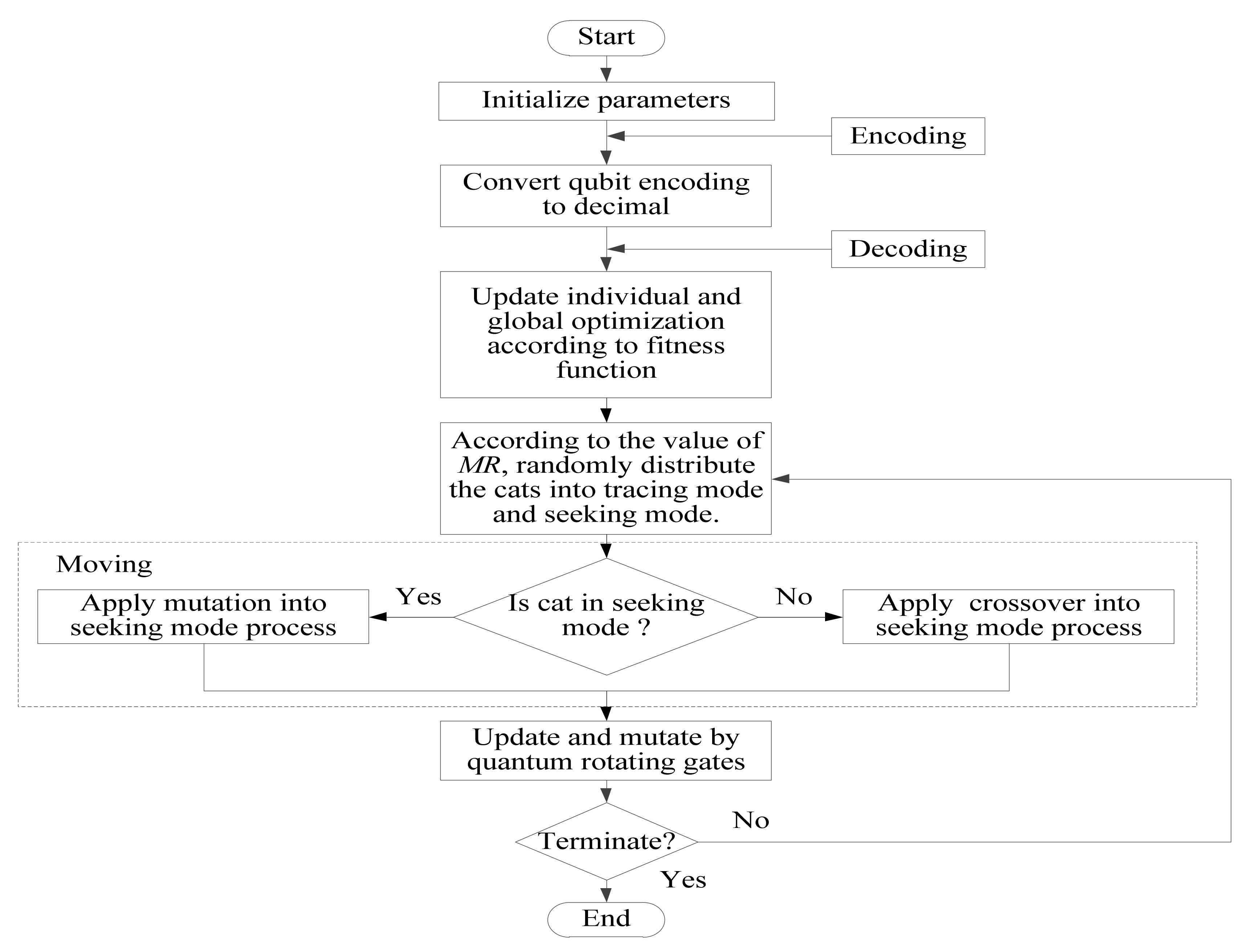
3.7. Flowchart of QCSO

The flow of QCSO is as follows:

① Initialize the population Q(t₀), and randomly create n chromosomes that encoded by qubit.

② Decode chromosomes and convert qubit encoding to decimal.

③ Measure each individual in initial population Q(t₀), and get a definite solution P(t₀).

④ Evaluate the fitness value of each solution, and save the optimal individual and its corresponding fitness value.

⑤ According to the value of MR, determine the individual searching and tracking status of the cat group, and judge whether the calculation process can be over. If the end condition is satisfied, then exit; otherwise, continue to calculate.

⑥ Measure each individual in population Q(t), and get the corresponding definite solution.

⑦ Evaluate the fitness value of each definite solution.

⑧ Use the quantum rotation gate G(t) to update the individual position of the cat swarm, and get the new population Q(t + 1).

⑨ Save the optimal cat swarm, optimal individual, and corresponding fitness value;

⑩ Increase the number of iterations by 1, and return to step ⑤.

The flowchart of the quantum cat swarm optimization algorithm is shown in Figure 1.

4. Algorithm Validation

4.1. Data Generation

This paper runs 2 × 4, 4 × 4, 4 × 6, 8 × 4, and 10 × 4 five-scale problems, in which every job has four procedures. For example, 8 × 4 indicates that there are eight kinds of jobs on four machines. The relevant data of the simulation analysis in this paper come from the literature [8], and each operation is processed on a different machine. Different processing times and setup times for the same machining tasks are scheduled on different machines, and the setup time matrix is asymmetric. Part of the data is shown in

Table 4. Optional machine table in each process of 4 × 4 problem.

Job	J1	J2	J3	J4
O1	1, 2	2	1, 2, 3	4
O2	2, 3	1, 4	3	1, 2
O3	3	1, 3	2, 3, 4	1, 2
O4	1, 2, 3	3	1	2, 4

,

Table 5. Processing time for 4 × 4 problem jobs (min).

Job	J1	J2	J3	J4
O1	87, 140	200, 220, 200	165, 150	1102.5, 1347.5, 1125
O2	210, 192	280, 260	165, 135, 165	1102.5, 1125, 1125
O3	245, 280, 262	240, 200	150, 180	1100, 1200
O4	245, 262	230, 270	140, 160	1000, 1050

,

Table 6. Initial setup time for 4 × 4 problem jobs (min).

Job	M1	M2	M3	M4
J1	220	90	80	45
J2	120	85	60	85
J3	235	75	65	127
J4	167	129	109	68

,

Table 7. Setup time for 4 × 4 problem jobs on M₁ (min).

Job	J1	J2	J3	J4
J1	0	250	176	155
J2	260	0	248	165
J3	210	50	0	218
J4	220	60	205	0

,

Table 8. Setup time for 4 × 4 problem jobs on M₂ (min).

Job	J1	J2	J3	J4
J1	0	190	161	292
J2	220	0	146	224
J3	260	122	0	158
J4	215	114	171	0

,

Table 9. Setup time for 4 × 4 problem jobs on M₃ (min).

Job	J1	J2	J3	J4
J1	0	235	231	285
J2	260	0	162	159
J3	290	193	0	202
J4	228	213	152	0

,

Table 10. Setup time for 4 × 4 problem jobs on M₄ (min).

Job	J1	J2	J3	J4
J1	0	252	203	252
J2	65	0	146	156
J3	154	68	0	159
J4	121	154	154	0

,

Table 11. Optional machine table in each process of 8 × 4 problem.

Job	J1	J2	J3	J4	J5	J6	J7	J8
O1	2, 3	1, 2, 4	2, 4	1, 2, 4	1, 2	1, 4	2, 3	4
O2	1, 3	1, 3	1, 2, 4	1, 2, 4	2, 4	2, 3	2, 3, 4	1, 2
O3	1, 2, 3	3, 4	1, 2	2, 4	1, 3, 4	1, 2, 3	1, 3	1, 2
O4	2, 4	1, 4	2, 3	2, 3	3,4	1	2, 4	1, 4

,

Table 12. Processing time for 8 × 4 problem jobs (min).

J1	J2	J3	J4
87, 140	200, 220, 200	165, 150	1102.5, 1347.5, 1125
210, 192.5	280, 260	165, 135, 165	1102.5, 1125, 1125
245, 280, 262.5	240, 200	150, 180	1100, 1200
245, 262.5	230, 270	140, 160	1000, 1050
J5	J6	J7	J8
220, 200	210, 240	180, 200	120
140, 120	260, 300	210, 235, 265	110, 160
180, 200, 220	200, 220, 260	250, 280	220, 260
130, 160	270	150, 180	200, 240

,

Table 13. Initial setup time for 8 × 4 problem jobs (min).

Job	M1	M2	M3	M4
J1	220	90	80	45
J2	120	85	60	85
J3	235	75	65	127
J4	167	129	109	68
J5	216	143	123	145
J6	134	110	95	187
J7	146	225	88	122
J8	221	219	75	157

,

Table 14. Setup time for 8 × 4 problem jobs on M₁ (min).

Job	J1	J2	J3	J4	J5	J6	J7	J8
J1	0	250	176	155	215	255	190	212
J2	260	0	248	165	223	157	154	214
J3	210	50	0	218	213	258	259	215
J4	220	60	205	0	119	159	164	227
J5	150	110	117	178	0	30	116	215
J6	130	125	129	132	137	0	40	203
J7	120	215	238	181	147	121	0	209
J8	150	225	159	169	116	212	113	0

,

Table 15. Setup time for 8 × 4 problem jobs on M₂ (min).

Job	J1	J2	J3	J4	J5	J6	J7	J8
J1	0	190	161	292	201	255	269	248
J2	220	0	146	224	209	157	254	218
J3	260	122	0	158	213	251	214	148
J4	215	114	171	0	151	220	207	214
J5	210	152	149	153	0	80	85	161
J6	159	155	219	159	156	0	90	142
J7	151	121	153	117	112	80	0	217
J8	154	216	165	152	119	210	159	0

,

Table 16. Setup time for 8 × 4 problem jobs on M₃ (min).

Job	J1	J2	J3	J4	J5	J6	J7	J8
J1	0	235	231	285	294	240	200	90
J2	260	0	162	159	221	100	200	60
J3	290	193	0	202	219	150	150	150
J4	228	213	152	0	55	118	159	208
J5	173	159	158	75	0	106	148	158
J6	119	156	159	206	149	0	157	204
J7	138	184	215	233	258	126	0	106
J8	176	217	208	259	239	137	125	0

and

Table 17. Setup time for 8 × 4 problem jobs on M₄ (min).

Job	J1	J2	J3	J4	J5	J6	J7	J8
J1	0	252	203	252	216	158	206	153
J2	65	0	146	156	101	212	103	157
J3	154	68	0	159	154	111	155	206
J4	121	154	154	0	35	108	203	108
J5	206	124	150	85	0	155	159	212
J6	151	158	104	104	203	0	95	203
J7	159	153	109	152	159	123	0	149
J8	107	152	112	101	206	109	45	0

. There is an initial setup time on each machine, which also differed. In the data tables, J_i refers to job I, O_j refers to operation j, J_ij refers to operation j of job i, and M_i refers to the machine number.

4.2. Calculation Result

In this paper, Matlab R2010a software was used in a PC with CORE i3 M 380 CPU, the main frequency of the CPU was 2.53 GHz, and the RAM was 500 GB. The relevant parameters of QCSO used in this paper refer to the literature [8,25]. The operation parameters were as follows: population size p = 60, termination algebra T = 200, dynamic rotation angle $\Delta \theta =0.15\pi ,0.16\pi ,0.2\pi$, and everyone was tested 20 times, SMP = 15, and MR varied randomly in the range [0.2, 0.8] according to the number of iterations of the algorithm. Further, c₁ = 2, r₁ is a random number in the range [0, 1]. The QCSO algorithm was compared to the parallel genetic algorithm (PGA) [8], and the comparison of calculation results included the following aspects: target minimum value (Min.sol), target average value (Avg.sol), target maximum value (Max.sol), times for optimal solution, average relative percentage error (RPE), and their standard deviation (SD). The percentage, which represents the absolute deviation of a measurement value to the mean value, is called RPE, and it is used to measure the deviation of a single measurement result from the mean value. SD is the square root of the sum of the squared deviation from the mean, and it is also the arithmetic square root of variance. It can reflect the discrete degree of the dataset, which is represented by σ. The smaller the value of σ, the better the stability of the algorithm. The formulas for RPE and σ are as follows:

$$RPE=\frac{C_{\max }^{PGA}-C_{\max }^{QCSO}}{C_{\max }^{QCSO}}\times 100$$

(19)

In Equation (19), $C_{\max }^{PGA}$ and $C_{\max }^{QCSO}$ indicate the optimization value of minimizing the makespan solved by PGA [8] and improved QCSO used in this paper.

$$\sigma =\sqrt{\frac{1}{N}{\displaystyle \sum _{i=1}^N{(x_i-\mu )}^2}}$$

(20)

In Equation (20), x_i are real numbers, and μ is the arithmetic mean value of x_i.

QCSO and PGA are used to solve different scale problems, and they were all run 20 times. It can be seen in

Table 18. Comparison results.

Problem scale: 2 × 4
	Max.sol (min)	Min.sol (min)	Avg.sol (min)	σ	Times for optimal solution
QCSO	1359	1359	1359	0	20
PGA	1359	1359	1359	0	20
Problem scale: 4 × 4
	Max.sol (min)	Min.sol (min)	Avg.sol (min)	σ	Times for optimal solution
QCSO	4773	4744	4761.4	10.58	18
PGA	4773	4744	4771.55	48	10
Problem scale: 6 × 4
	Max.sol (min)	Min.sol (min)	Avg.sol (min)	σ	Times for optimal solution
QCSO	4924	4764	47945	20.57	16
PGA	4854	4764	4784.35	25.93	14
Problem scale: 8 × 4
	Max.sol (min)	Min.sol (min)	Avg.sol (min)	σ	Times for optimal solution
QCSO	5118	4853	4941.2	62.48	16
PGA	5184	4826	4962.8	1103	12
Problem scale: 10 × 4
	Max.sol (min)	Min.sol (min)	Avg.sol (min)	σ	Times for optimal solution
QCSO	5590	5234	5444.3	91.81	15
PGA	5954	5164	5607	192.51	8

that there is little difference in the optimization ability of the two algorithms when the scale of the problem is relatively small, but when the scale of the problem increases, the optimization ability of QCSO is obviously better than that of PGA. Although the average difference of the optimal solution is not very large, the SD contrast is obvious. For the 8 × 4 problem scale, σ calculated by QCSO is 62.48 and by PGA is 1103, and the difference is 53.55. For the 10 × 4 problem scale, σ calculated by QCSO is 91.81 and by PGA is 192.51, and the difference is 100.7. This illustrates that when the scale of the problem increases, QCSO is better than PGA. In addition, the results of running it 20 times show that with increased problem scale, QCSO searches for the optimal solution more times than PGA. For example, for the 6 × 4 problem scale, the ratio of times QCSO searched for the optimal solution is 80%, while the ratio for PGA is 70%. For the 8 × 4 problem scale, the ratio of times QCSO searched for optimal solution is 80%, but the ratio for PGA is 60%. For the 10 × 4 problem scale, the ratio of times QCSO searched for the optimal solution is 75%, while the ratio for PGA is 40%. All of this shows that the stability of QCSO is better.

Twenty RPE values of different scale problems running results are shown in

Table 19. RPE values of different scale problem running results.

n	m	Instance	RPE	n	m	Instance	RPE	n	m	Instance	RPE
6	4	1	−0.13	8	4	1	2.09	10	4	1	1.03
		2	0			2	0.35			2	−4.55
		3	0.69			3	−1.37			3	50
		4	−0.10			4	4.38			4	5.72
		5	0			5	−1.45			5	1.17
		6	2.64			6	1.39			6	2.52
		7	0.92			7	5.83			7	−3.08
		8	−1.45			8	3.62			8	2.78
		9	0.19			9	3.77			9	9.37
		10	1.55			10	1.94			10	−1.16
		11	0.02			11	5.67			11	5.51
		12	0.11			12	0.66			12	0.78
		13	−0.12			13	0.16			13	3.86
		14	−1.12			14	7.09			14	4.31
		15	−0.21			15	1.42			15	7.44
		16	3.27			16	−0.80			16	80
		17	−0.13			17	4.33			17	−0.71
		18	−1.02			18	0.37			18	2.46
		19	−0.10			19	1.45			19	0.82
		20	0.10			20	0.16			20	2.36
		Mean	0.26			Mean	2.05			Mean	2.70

. The mean values of RPE for three kinds of scale problems are all positive, indicating that QCSO is significantly better than PGA, and QCSO is improved by about 2% on average. The analysis in this paper shows that the improved QCSO algorithm introduces quantum coding, which expands the ergodicity of the algorithm. By renewing the quantum rotation angle, the position of the cat swarm is iteratively updated, and the search efficiency and running speed of the algorithm are improved. MR, the number of cats that execute tracing mode, accounting for a proportion of the entire cat swarm, is set to a range of [0.2, 0.8] in this paper. It varies dynamically according to the change in iteration number of the algorithm, which improves its optimization capability.

The 6 × 4, 8 × 4, and 10 × 4 problem working sketches solved using QCSO and PGA are shown in Figure 2, Figure 3 and Figure 4, respectively, and the number of iterations for all of them is 20. It is confirmed that the convergence speed and the stability of QCSO is better, especially for solving large-scale problems. Gantt charts of optimal solutions for the 6 × 4, 8 × 4, and 10 × 4 problems based on QCSO are shown in Figure 5, Figure 6 and Figure 7, respectively; the numbers on the colored progress bars represent the procedure of the job. For example, in Figure 7, 101 on the first progress bar of the second line indicates that the first operation of the first job is arranged to be processed on machine 3. The space between the colored progress bars on each line is the setup time, and its size indicates the length of the setup time. The space in front of the job operation ranked first on each machine represents the initial setup time of that machine.

5. Conclusions

To improve production efficiency, reduce cost, and increase the flexible production of the job-shop, each operation of the same job can be processed on a different machine, and the processing and setup times of the same operation on the different machines are not the same. Different job sequences on the same machine result in different setup times, and because of the extremely low repetition rate of single-item and small-batch products, it is impossible to obtain setup times for different processing sequences. To shorten the setup times and improve the utilization rate of equipment and other resources, in this paper we examine a job-shop scheduling optimization scheme based on group technology. First, we cluster the job into groups according to the similarity of the required processing resources. Second, we select the processing machines according to the machine load and processing time. Finally, we schedule the procedures on the machines with the optimization objective of minimizing the completion time according to the setup and processing time. In this paper, we combine qubit and QCSO and propose the improved QCSO to solve the FJSP. We also introduce quantum coding, which extends the ergodicity of the algorithm. By renewing the quantum rotation angle, the position of the cat swarm is iteratively updated, and the operation efficiency and speed of the algorithm are improved. Dynamic MR values in the range of [0.2, 0.8] are used in this paper, which vary randomly according to the number of iterations of the algorithm. Finally, the operation results of the improved QCSO and PGA are compared through simulation experiments [8], and the minimum, average, and maximum values of the objective function, relative percentage deviation, and standard deviation are compared. The results show that the improved QCSO has better optimization results and robustness, and these results confirm the feasibility and validity of the method used in this paper.

References

1. Wolpert, D.H.; Macready, W.G. No free lunch theorems for optimization. IEEE Trans. Evol. Comput. 1997, 1, 67–82. [Google Scholar] [CrossRef] [Green Version]
2. Mousakhani, M. Sequence-dependent setup time flexible job-shop scheduling problem to minimise total tardiness. Int. J. Prod. Res. 2013, 51, 3476–3487. [Google Scholar] [CrossRef]
3. Shen, L.; Dauzère-Pérès, S.; Neufeld, J.S. Solving the flexible job-shop scheduling problem with sequence-dependent setup times. Eur. J. Oper. Res. 2018, 265, 503–516. [Google Scholar] [CrossRef]
4. Bagheri, A.; Zandieh, M. Bi-criteria flexible job-shop scheduling with sequence-dependent setup times—Variable neighborhood search approach. J. Manuf. Syst. 2011, 30, 8–15. [Google Scholar] [CrossRef]
5. Abdelmaguid, T.F. A neighborhood search function for flexible job-shop scheduling with separable sequence-dependent setup times. Appl. Math. Comput. 2015, 260, 188–203. [Google Scholar] [CrossRef]
6. Naderi, B.; Zandieh, M.; Fatemi Ghomi, S.M.T. Scheduling job-shop problems with sequence-dependent setup times. Int. J. Prod. Res. 2009, 47, 5959–5976. [Google Scholar] [CrossRef]
7. Li, M.; Lei, D. An imperialist competitive algorithm with feedback for energy-efficient flexible job shop scheduling with transportation and sequence-dependent setup times. Eng. Appl. Artif. Intell. 2021, 103, 104307. [Google Scholar] [CrossRef]
8. Defersha, F.M.; Chen, M. A parallel genetic algorithm for a flexible job-shop scheduling problem with sequence dependent setups. Int. J. Adv. Manuf. Technol. 2010, 49, 263–279. [Google Scholar] [CrossRef]
9. Azzouz, A.; Ennigrou, M.; Ben Said, L. A hybrid algorithm for flexible job-shop scheduling problem with setup times. Int. J. Prod. Manag. Eng. 2017, 5, 23–30. [Google Scholar] [CrossRef] [Green Version]
10. Wang, Y.; Zhu, Q. A Hybrid Genetic Algorithm for Flexible Job-shop Scheduling Problem with Sequence-Dependent Setup Times and Job Lag Times. IEEE Access 2021, 9, 104864–104873. [Google Scholar] [CrossRef]
11. Li, Z.C.; Qian, B.; Hu, R. An elitist nondominated sorting hybrid algorithm for multi-objective flexible job-shop scheduling problem with sequence-dependent setups. Knowl. Based Syst. 2019, 173, 83–112. [Google Scholar] [CrossRef]
12. Azzouz, A.; Ennigrou, M.; Said, L.B. A self-adaptive hybrid algorithm for solving flexible job-shop problem with sequence dependent setup time. Procedia Comput. Sci. 2017, 112, 457–466. [Google Scholar] [CrossRef]
13. Azzouz, A.; Ennigrou, M.; Said, L.B. Solving flexible job-shop problem with sequence dependent setup time and learning effects using an adaptive genetic algorithm. Int. J. Comput. Intell. Stud. 2020, 9, 18–32. [Google Scholar] [CrossRef]
14. Abderrabi, F.; Godichaud, M.; Yalaoui, A. Flexible Job-shop Scheduling Problem with Sequence Dependent Setup Time and Job Splitting: Hospital Catering Case Study. Appl. Sci. 2021, 11, 1504. [Google Scholar] [CrossRef]
15. Parjapati, S.K.; Ajai, J. Optimization of flexible job-shop scheduling problem with sequence dependent setup times using genetic algorithm approach. Int. J. Math. Comput. Nat. Phys. Eng. 2015, 9, 41–47. [Google Scholar]
16. Sadrzadeh, A. Development of both the AIS and PSO for solving the flexible job-shop scheduling problem. Arab. J. Sci. Eng. 2013, 38, 3593–3604. [Google Scholar] [CrossRef]
17. Tayebi Araghi, M.E.; Jolai, F.; Rabiee, M. Incorporating learning effect and deterioration for solving a SDST flexible job-shop scheduling problem with a hybrid heuristic approach. Int. J. Comput. Integr. Manuf. 2014, 27, 733–746. [Google Scholar] [CrossRef]
18. Sun, J.; Zhang, G.; Lu, J. A hybrid many-objective evolutionary algorithm for flexible job-shop scheduling problem with transportation and setup times. Comput. Oper. Res. 2021, 132, 105263. [Google Scholar] [CrossRef]
19. Li, J.; Deng, J.; Li, C. An improved Jaya algorithm for solving the flexible job-shop scheduling problem with transportation and setup times. Knowl. Based Syst. 2020, 200, 106032. [Google Scholar] [CrossRef]
20. Raj, S.; Bhattacharyya, B. Reactive power planning by opposition-based grey wolf optimization method. Int. Trans. Electr. Energy Syst. 2018, 28, 1–17. [Google Scholar] [CrossRef]
21. Wei, Z.; Liao, W.; Zhang, L. Hybrid energy-efficient scheduling measures for flexible job-shop problem with variable machining speeds. Expert Syst. Appl. 2022, 197, 116785. [Google Scholar] [CrossRef]
22. Li, R.; Gong, W.; Lu, C. Self-adaptive multi-objective evolutionary algorithm for flexible job shop scheduling with fuzzy processing time. Comput. Ind. Eng. 2022, 168, 108099. [Google Scholar] [CrossRef]
23. Türkyılmaz, A.; Senvar, O.; Ünal, İ. A hybrid genetic algorithm based on a two-level hypervolume contribution measure selection strategy for bi-objective flexible job shop problem. Comput. Oper. Res. 2022, 141, 105694. [Google Scholar] [CrossRef]
24. Jiang, X.; Tian, Z.; Liu, W. Energy-efficient scheduling of flexible job shops with complex processes: A case study for the aerospace industry complex components in China. J. Ind. Inf. Integr. 2022, 27, 100293. [Google Scholar] [CrossRef]
25. Raj, S.; Bhattacharyya, B. Optimal placement of TCSC and SVC for reactive power planning using Whale optimization algorithm. Swarm Evol. Comput. 2018, 40, 131–143. [Google Scholar] [CrossRef]
26. Shiva, C.K.; Gudadappanavar, S.S.; Vedik, B. Fuzzy-Based Shunt VAR Source Placement and Sizing by Oppositional Crow Search Algorithm. J. Control. Autom. Electr. Syst. 2022. [Google Scholar] [CrossRef]
27. Chu, S.C.; Tsai, P.W. Computational intelligence based on the behavior of cats. Int. J. Innov. Comput. Inf. Control. 2007, 3, 163–173. [Google Scholar]
28. Guo, L.; Meng, Z.; Sun, Y. Parameter identification and sensitivity analysis of solar cell models with cat swarm optimization algorithm. Energy Convers. Manag. 2016, 108, 520–528. [Google Scholar] [CrossRef]
29. Orouskhani, M.; Orouskhani, Y.; Mansouri, M. A novel cat swarm optimization algorithm for unconstrained optimization problems. Int. J. Inf. Technol. Comput. Sci. 2013, 5, 32–41. [Google Scholar] [CrossRef]
30. Lin, K.C.; Zhang, K.Y.; Huang, Y.H. Feature selection based on an improved cat swarm optimization algorithm for big data classification. J. Supercomput. 2016, 72, 3210–3221. [Google Scholar] [CrossRef]
31. Kumar, Y.; Singh, P.K. Improved cat swarm optimization algorithm for solving global optimization problems and its application to clustering. Appl. Intell. 2018, 48, 2681–2697. [Google Scholar] [CrossRef]
32. Kong, L.; Pan, J.S.; Tsai, P.W. A balanced power consumption algorithm based on enhanced parallel cat swarm optimization for wireless sensor network. Int. J. Distrib. Sens. Netw. 2015, 11, 1–10. [Google Scholar] [CrossRef] [Green Version]
33. Skoullis, V.I.; Tassopoulos, I.X.; Beligiannis, G.N. Solving the high school timetabling problem using a hybrid cat swarm optimization based algorithm. Appl. Soft Comput. 2017, 52, 277–289. [Google Scholar] [CrossRef]
34. Huang, J.D.; Asteris, P.G.; Pasha, S.M.K. A new auto-tuning model for predicting the rock fragmentation: A cat swarm optimization algorithm. Eng. Comput. 2022, 38, 2209–2220. [Google Scholar] [CrossRef]
35. Sikkandar, H.; Thiyagarajan, R. Deep learning based facial expression recognition using improved Cat Swarm Optimization. J. Ambient. Intell. Humaniz. Comput. 2021, 12, 3037–3053. [Google Scholar] [CrossRef]
36. Yan, D.; Cao, H.; Yu, Y. Single- objective/multi -objective cat swarm optimization clustering analysis for data partition. IEEE Trans. Autom. Sci. Eng. 2020, 17, 1633–1646. [Google Scholar]
37. Singh, H.; Kumar, Y. A neighborhood search-based cat swarm optimization algorithm for clustering problems. Evol. Intell. 2020, 13, 593–609. [Google Scholar] [CrossRef]
38. Zhang, J. Modified Quantum Evolutionary Algorithms for Scheduling Problems. Ph.D. Thesis, East China University of Science and Technology, Hanghai, China, 2013. [Google Scholar]
Figure 1. Flowchart of quantum cat swarm optimization algorithm.
Sustainability 14 09547 g001
Figure 2. QCSO and PGA used to solve 6 × 4 problem working sketch. (a) QCSO used to solve 6 × 4 problem working sketch. (b) PGA used to solve 6 × 4 problem working sketch.
Sustainability 14 09547 g002
Figure 3. QCSO and PGA to solve 8 × 4 problem working sketch. (a) QCSO used to solve 8 × 4 problem working sketch (b) PGA used to solve 8 × 4 problem working sketch.
Sustainability 14 09547 g003
Figure 4. QCSO and PGA to solve 10 × 4 problem working sketch. (a) QCSO used to solve 10 × 4 problem working sketch (b) PGA used to solve 10 × 4 problem working sketch.
Sustainability 14 09547 g004
Figure 5. Gantt chart of optimal solution to 6 × 4 problem using QCSO.
Sustainability 14 09547 g005
Figure 6. Gantt chart of optimal solution to 8 × 4 problem using QCSO.
Sustainability 14 09547 g006
Figure 7. Gantt chart of optimal solution to 10 × 4 problem using QCSO.
Sustainability 14 09547 g007