
Study on Urban Thermal Environment in Beijing Based on Local Climate Zone Method


Abstract
:1. Introduction
2. Data and Methods
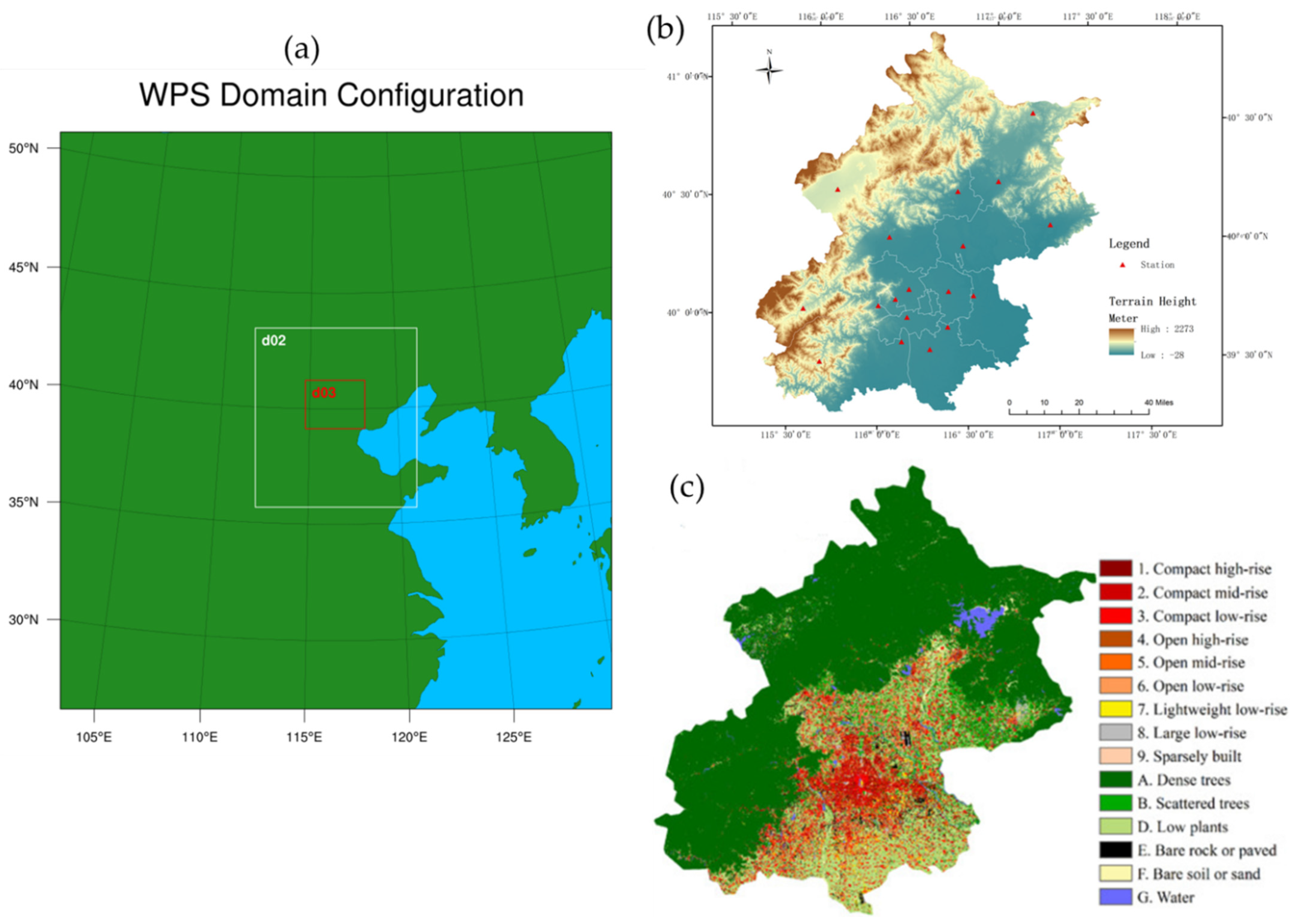
2.1. Study Area
2.2. Data
2.3. Design of Numerical Test Scheme
2.4. Mode Evaluation Method
2.5. The Urban Heat Island Effect
3. Results
3.1. Analysis of 2 m Daily Temperature Variation
3.2. Spatial Distribution Analysis of Thermal Environment
3.2.1. Spatial Distribution Analysis of 2 m Temperature
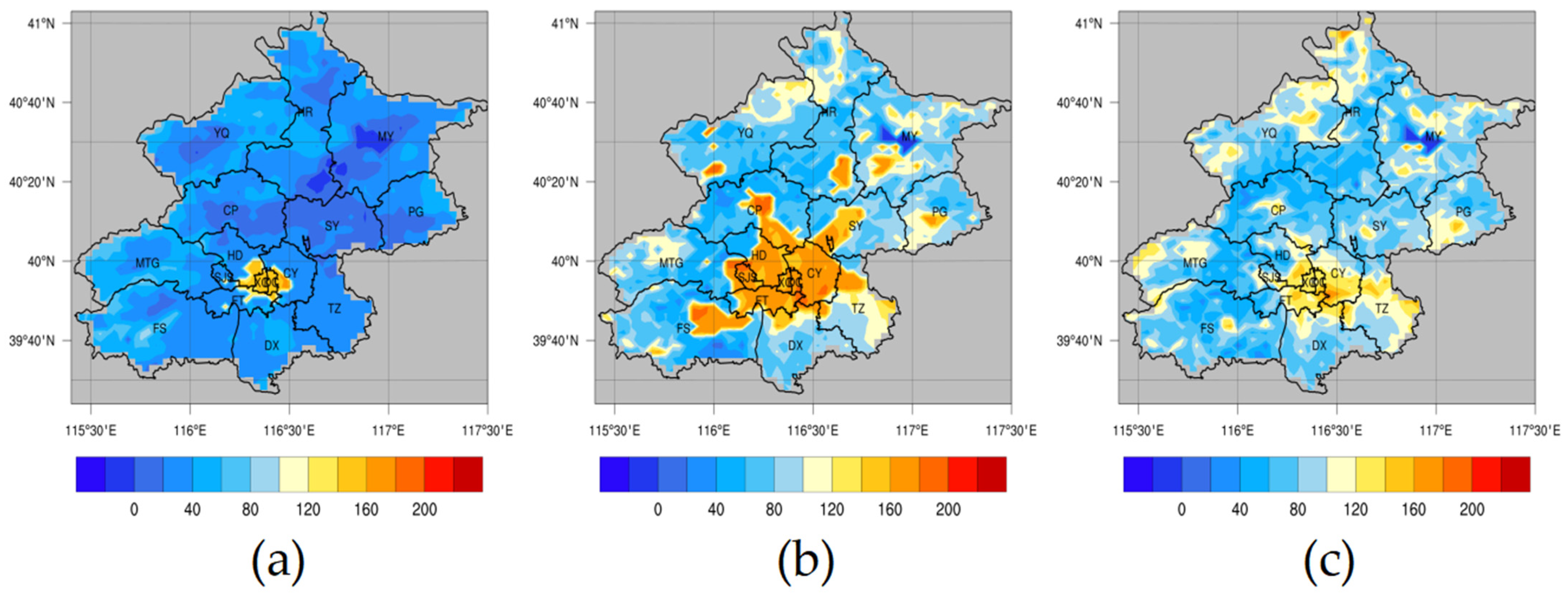
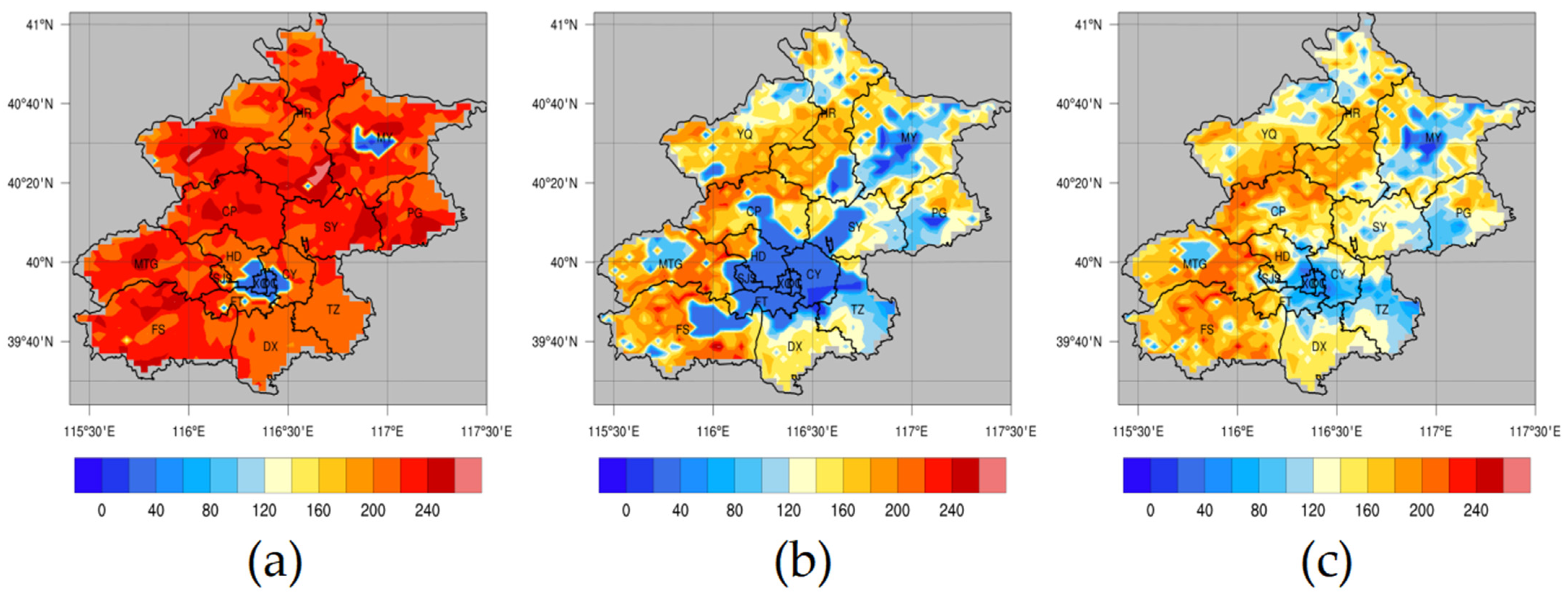
3.2.2. Spatial Distribution Analysis of Surface Heat Flux
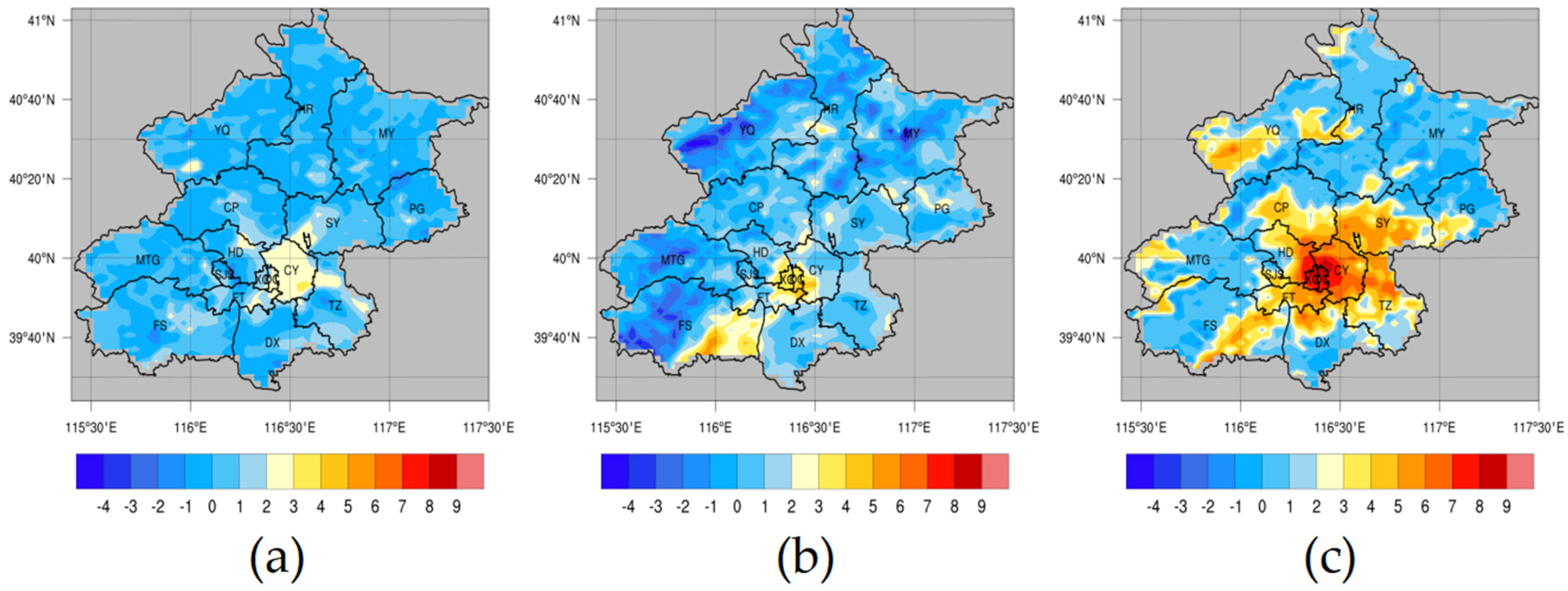
3.2.3. Heat Island Intensity Distribution
3.3. Influence of Urbanization Development on 2 m Temperature in Beijing
4. Discussion
5. Conclusions
- Our research results show that the simulated 2 m temperature of the scheme of correcting only urban areas is the closest to the observed data, with an R of 0.93, an RMSE of 1.84 °C, and an MAE of 0.01 °C. There is a close relationship between the simulated results of the LCZ scheme and the types of the underlying surface. For example, the UR1 station is classified as open low-rise built, and the simulated result of the 2 m temperature is closer to the observed data than the MODIS scheme and scheme of correcting only urban areas.
- The MODIS scheme, the scheme of correcting only urban areas, and the LCZ scheme can simulate the diurnal variation characteristics of temperature. Although the RMSE in the 2 m temperature simulated by the LCZ scheme is 0.43 °C higher than that of the scheme of correcting only urban areas, it can well reproduce the spatial variation characteristics of the 2 m temperature.
- For the simulation of the surface heat flux, the sensible heat value of the scheme of correcting only urban areas has an obvious high-value center, and the latent heat value gradient is too large at the boundary between urban and rural areas, which forms an unreasonable mutation in the space. In the LCZ scheme, the sensible heat has no obvious high-value center, showing a linear band distribution of increasing sensible heat from the northwest to southeast, and the latent heat distribution is more reasonable. The low latent heat area is located in the Xicheng and Dongcheng areas, which is also the location of the core area of Beijing, and with the built-up area spreading out around the Xicheng and Dongcheng District as the center, the latent heat value increases slowly.
- Urban heat islands exist day and night in Beijing, and the intensity at night is much higher than that in the daytime. The total urban area in land use data affects the intensity and distribution of the heat island, and the difference in the urban internal division has a significant impact on the heat island. High-temperature heat island areas are mainly concentrated in compact low-level, compact mid-level, and large low-level types.
- In the study of the impact of urbanization on the 2 m temperature, the LCZ scheme can more clearly reflect the temperature difference within urban areas.
Author Contributions
Funding
Institutional Review Board Statement
Informed Consent Statement
Data Availability Statement
Acknowledgments
Conflicts of Interest
References
- Zhang, H.; Wu, C.; Chen, W.; Huang, G. Effect of urban expansion on summer rainfall in the Pearl River Delta. J. Hydrol. 2019, 568, 747–757. [Google Scholar] [CrossRef]
- Akbari, H.; Kolokotsa, D. Three decades of urban heat islands and mitigation technologies research. Energy Build. 2016, 133, 834–842. [Google Scholar] [CrossRef]
- Liao, J.; Wang, T.; Jiang, Z.; Zhuang, B.; Xie, M.; Yin, C.; Wang, X.; Zhu, J.; Fu, Y.; Zhang, Y. WRF/Chem modeling of the impacts of urban expansion on regional climate and air pollutants in Yangtze River Delta. Atmos. Environ. 2015, 106, 204–214. [Google Scholar] [CrossRef]
- Wang, W.; Ng, E. Air ventilation assessment under unstable atmospheric stratification—A comparative study for Hong Kong. Build. Environ. 2018, 130, 1–13. [Google Scholar] [CrossRef]
- Bonczak, B.; Kontokosta, C.E. Large-scale parameterization of 3D building morphology in complex urban landscapes using aerial LiDAR and city administrative data. Comput. Environ. Urban. Syst. 2019, 73, 126–142. [Google Scholar] [CrossRef]
- Dai, J.; Wang, X.; Dai, W.; Chang, M. The impact of inhomogeneous urban canopy parameters on meteorological conditions and implication for air quality in the Pearl River Delta region. Urban. Clim. 2019, 29, 100494. [Google Scholar] [CrossRef]
- Lai, X.; Li, M.; Liu, C.; Zhong, Y.; Lin, L.; Wang, H. The phenological responses of plants to the heat island effect in the main urban area of Chongqing. Acta Ecol. Sin. 2019, 39, 7025–7034. [Google Scholar]
- Jiang, W.; Li, J.; Chen, Y. An Approach to Relationship between Urban Wetland and Urban Heat Island Effect. Shanghai Environ. Sci. 2007, 26, 151–155. [Google Scholar]
- Sharma, A.; Conry, P.; Fernando, H.J.S.; Hamlet, A.F.; Hellmann, J.J.; Chen, F. Green and cool roofs to mitigate urban heat island effects in the chicago metropolitan area: Evaluation with a regional climate model. Environ. Res. Lett. 2016, 11, 064004. [Google Scholar] [CrossRef]
- Skamarock, C.; Klemp, B.; Dudhia, J.; Gill, O.; Liu, Z.; Berner, J.; Wang, W.; Powers, G.; Duda, G.; Barker, D.M.; et al. A Description of the Advanced Research WRF Model Version 4. NCAR Tech. 2021, 113, 7–25. [Google Scholar]
- Chang, M.; Fan, S.; Wang, X. Impact of refined land-cover data on WRF performance over the Pearl River Delta region. Acta Sci. Circumstantiae 2014, 34, 1922–1933. [Google Scholar]
- Zhang, N.; Wang, X.; Chen, Y.; Dai, W.; Wang, X. Numerical simulations on influence of urban land cover expansion and anthropogenic heat release on urban meteorological environment in Pearl River Delta. Theor. Appl. Climatol. 2016, 126, 469–479. [Google Scholar] [CrossRef]
- Stewart, I.D.; Oke, T.R. Local Climate Zones for Urban Temperature Studies. Bull. Am. Meteorol. Soc. 2012, 93, 1879–1900. [Google Scholar] [CrossRef]
- Brousse, O.; Martilli, A.; Foley, M.; Mills, G.; Bechtel, B. WUDAPT, an efficient land use producing data tool for mesoscale models? Integration of urban LCZ in WRF over Madrid. Urban. Clim. 2016, 17, 116–134. [Google Scholar] [CrossRef]
- Mu, Q.; Miao, S.; Wang, Y.; Li, Y.; Yan, C. Evaluation of employing local climate zone classification for mesoscale modelling over Beijing metropolitan area. Meteorol. Atmos. Phys. 2020, 132, 315–326. [Google Scholar] [CrossRef]
- Mughal, M.O.; Li, X.-X.; Yin, T.; Martilli, A.; Brousse, O.; Dissegna, M.A.; Norford, L.K. High-Resolution, Multilayer Modeling of Singapore’s Urban Climate Incorporating Local Climate Zones. J. Geophys. Res. Atmospheres. 2019, 124, 7764–7785. [Google Scholar] [CrossRef]
- Molnar, G.; Gyongyosi, A.Z.; Gal, T. Integration of an LCZ-based classification into WRF to assess the intra-urban temperature pattern under a heatwave period in Szeged. Theor. Appl. Climatol. 2019, 138, 1139–1158. [Google Scholar] [CrossRef] [Green Version]
- Pellegatti Franco, D.M.; Andrade, M.d.F.; Ynoue, R.Y.; Ching, J. Effect of Local Climate Zone (LCZ) classification on ozone chemical transport model simulations in Sao Paulo, Brazil. Urban. Clim. 2019, 27, 293–313. [Google Scholar] [CrossRef]
- Patel, P.; Karmakar, S.; Ghosh, S.; Niyogi, D. Improved simulation of very heavy rainfall events by incorporating WUDAPT urban land use/land cover in WRF. Urban. Clim. 2020, 32, 100616. [Google Scholar] [CrossRef]
- Chen, F.; Kusaka, H.; Bornstein, R.; Ching, J.; Grimmond, C.S.B.; Grossman-Clarke, S.; Loridan, T.; Manning, K.W.; Martilli, A.; Miao, S.; et al. The integrated WRF/urban modelling system: Development, evaluation, and applications to urban environmental problems. Int. J. Climatol. 2011, 31, 273–288. [Google Scholar] [CrossRef]
- Salamanca, F.; Martilli, A. A new Building Energy Model coupled with an Urban Canopy Parameterization for urban climate simulations-part II. Validation with one dimension off-line simulations. Theor. Appl. Climatol. 2010, 99, 345–356. [Google Scholar] [CrossRef]
- Kusaka, H.; Kondo, H.; Kikegawa, Y.; Kimura, F. A simple single-layer urban canopy model for atmospheric models: Comparison with multi-layer and slab models. Bound. Layer Meteorol. 2001, 101, 329–358. [Google Scholar] [CrossRef]
- Sharma, A.; Fernando, H.J.S.; Hamlet, A.F.; Hellmann, J.J.; Barlage, M.; Chen, F. Urban meteorological modeling using WRF: A sensitivity study. Int. J. Climatol. 2017, 37, 1885–1900. [Google Scholar] [CrossRef]
- Giannaros, C.; Nenes, A.; Giannaros, T.M.; Kourtidis, K.; Melas, D. A comprehensive approach for the simulation of the Urban Heat Island effect with the WRF/SLUCM modeling system: The case of Athens (Greece). Atmos. Res. 2018, 201, 86–101. [Google Scholar] [CrossRef]
- Huang, M.; Gao, Z.; Miao, S.; Chen, F. Sensitivity of urban boundary layer simulation to urban canopy models and PBL schemes in Beijing. Meteorol. Atmos. Phys. 2019, 131, 1235–1248. [Google Scholar] [CrossRef]
- Bueno, B.; Roth, M.; Norford, L.; Li, R. Computationally efficient prediction of canopy level urban air temperature at the neighbourhood scale. Urban. Clim. 2014, 9, 35–53. [Google Scholar] [CrossRef] [Green Version]
- Salvati, A.; Coch Roura, H.; Cecere, C. Assessing the urban heat island and its energy impact on residential buildings in Mediterranean climate: Barcelona case study. Energy Build. 2017, 146, 38–54. [Google Scholar] [CrossRef] [Green Version]
- Detommaso, M.; Costanzo, V.; Nocera, F. Application of weather data morphing for calibration of urban ENVI-met microclimate models. Results and critical issues. Urban. Clim. 2021, 38, 100895. [Google Scholar] [CrossRef]
- Detommaso, M.; Gagliano, A.; Marletta, L.; Nocera, F. Sustainable Urban Greening and Cooling Strategies for Thermal Comfort at Pedestrian Level. Sustainability 2021, 13, 3138. [Google Scholar] [CrossRef]
- Macintyre, H.L.; Heaviside, C. Potential benefits of cool roofs in reducing heat-related mortality during heatwaves in a European city. Environ. Int. 2019, 127, 430–441. [Google Scholar] [CrossRef]
- Kolokotsa, D.; Santamouris, M.; Zerefos, S.C. Green and cool roofs’ urban heat island mitigation potential in European climates for office buildings under free floating conditions. Sol. Energy 2013, 95, 118–130. [Google Scholar] [CrossRef]
- Pyrgou, A.; Castaldo, V.L.; Pisello, A.L.; Cotana, F.; Santamouris, M. On the effect of summer heatwaves and urban overheating on building thermal-energy performance in central Italy. Sustain. Cities Soc. 2017, 28, 187–200. [Google Scholar] [CrossRef]
- Santamouris, M. Cooling the cities—A review of reflective and green roof mitigation technologies to fight heat island and improve comfort in urban environments. Sol. Energy 2014, 103, 682–703. [Google Scholar] [CrossRef]
- Touchaei, A.G.; Hosseini, M.; Akbari, H. Energy savings potentials of commercial buildings by urban heat island reduction strategies in Montreal (Canada). Energy Build. 2016, 110, 41–48. [Google Scholar] [CrossRef]
- Chen, B.; Wang, W.; Dai, W.; Chang, M.; Wang, X.; You, Y.; Zhu, W.; Liao, C. Refined urban canopy parameters and their impacts on simulation of urbanization-induced climate change. Urban. Clim. 2021, 37, 100847. [Google Scholar] [CrossRef]
- Ching, J.; Aliaga, D.; Mills, G.; Masson, V.; See, L.; Neophytou, M.; Middel, A.; Baklanov, A.; Ren, C.; Ng, E.; et al. Pathway using WUDAPT’s Digital Synthetic City tool towards generating urban canopy parameters for multi-scale urban atmospheric modeling. Urban. Clim. 2019, 28, 100459. [Google Scholar] [CrossRef]
- Ren, C.; Cai, M.; Li, X.; Zhang, L.; Wang, R.; Xu, Y.; Ng, E. Assessment of Local Climate Zone Classification Maps of Cities in China and Feasible Refinements. Sci. Rep. 2019, 9, 18848. [Google Scholar] [CrossRef] [Green Version]
- Jimenez, P.A.; Dudhia, J.; Gonzalez-Rouco, J.F.; Navarro, J.; Montavez, J.P.; Garcia-Bustamante, E. A Revised Scheme for the WRF Surface Layer Formulation. Mon. Weather. Rev. 2012, 140, 898–918. [Google Scholar] [CrossRef] [Green Version]
- Fairall, C.W.; Bradley, E.F.; Hare, J.E.; Grachev, A.A.; Edson, J.B. Bulk parameterization of air-sea fluxes: Updates and verification for the COARE algorithm. J. Clim. 2003, 16, 571–591. [Google Scholar] [CrossRef]
- Lim, J.-O.J.; Hong, S.-Y. The WRF Single-Moment 6-Class Microphysics Scheme (WSM6). Asia-Pac. J. Atmos. Sci. 2006, 42, 129–151. [Google Scholar]
- Mlawer, E.J.; Taubman, S.J.; Brown, P.D.; Iacono, M.J.; Clough, S.A. Radiative transfer for inhomogeneous atmospheres: RRTM, a validated correlated-k model for the longwave. J. Geophys. Res. Atmospheres. 1997, 102, 16663–16682. [Google Scholar] [CrossRef] [Green Version]
- Dudhia, J. Numerical Study of Convection Observed during the Winter Monsoon Experiment Using a Mesoscale Two-Dimensional Model. J. Atmos. Sci. 1989, 46, 3077–3107. [Google Scholar] [CrossRef]
- Kain, J.S. The Kain-Fritsch convective parameterization: An update. J. Appl. Meteorol. 2004, 43, 170–181. [Google Scholar] [CrossRef] [Green Version]
- Hong, S.-Y.; Noh, Y.; Dudhia, J. A new vertical diffusion package with an explicit treatment of entrainment processes. Mon. Weather. Rev. 2006, 134, 2318–2341. [Google Scholar] [CrossRef] [Green Version]
- Liang, T.; Chen, L.; He, J.; Zhang, L.; Gong, S.; Che, H. Study of Sensitivity Simulation of Planetary Boundary Layer Parameterization Schemes in Beijing. Plateau Meteorol. 2021, 40, 656–670. [Google Scholar]
- Chen, F.; Yang, X.; Zhu, W. WRF simulations of urban heat island under hot-weather synoptic conditions: The case study of Hangzhou City, China. Atmos. Res. 2014, 138, 364–377. [Google Scholar] [CrossRef]
- Mughal, M.O.; Li, X.-X.; Yin, T.; Martilli, A.; Brousse, O.; Dissegna, M.A.; Norford, L.K. Reply to Comment by Velasco on ‘High-Resolution, Multilayer Modeling of Singapore’s Urban Climate Incorporating Local Climate Zones’. J. Geophys. Res. Atmospheres 2021, 126, e2020JD034160. [Google Scholar] [CrossRef]
- Liang, T.; He, J.; Chen, L.; Yao, Z.; Zhang, L.; Che, H.; Gong, S. Simulation of the influence of a fine-scale urban underlying surface on the urban heat island effect in Beijing. Atmos. Res. 2021, 262, 105786. [Google Scholar] [CrossRef]
- Hu, J.; Chen, L. Influence of Land Use Data Optimization Schemes on WRF Model Simulations of High Temperature Processes in Shanghai. Clim. Environ. Res. 2020, 25, 443–456. [Google Scholar]
- Cai, Z.; Tang, Y.; Liu, C.; Matthias, D. Analyzing the Transformation of 3D Urban Morphology and Corresponding Surface Heat Island Effect in Beijing. Urban. Plan. Int. 2021, 36, 61–68. [Google Scholar]


| d01 | d02 | d03 | |
|---|---|---|---|
| Microphysical processes | Wsm6 simple ice scheme | Wsm6 simple ice scheme | Wsm6 simple ice scheme |
| Long-wave radiation | RRTM | RRTM | RRTM |
| Short-wave radiation | Dudhia | Dudhia | Dudhia |
| Near surface layer | Revised MM5 | Revised MM5 | Revised MM5 |
| Land surface process | Noah scheme | Noah scheme | Noah scheme |
| boundary layer | Ysu scheme | Ysu scheme | Ysu scheme |
| Cumulus parameterization | Kain–Fritsch | Kain–Fritsch | Kain–Fritsch |
| Case Name | Case 1 | Case 2 | Case 3 |
|---|---|---|---|
| Underlying surface information | MODIS scheme | Scheme of correcting only urban area | Local climate zone scheme |
| Number of urban internal classifications | 1 | 1 | 9 |
| Urban canopy model | BEM | BEM | BEM |
| Station ID | Station Name | Land Use Classification | ||
|---|---|---|---|---|
| Case 1 | Case 2 | Case 3 | ||
| UR1 | Shunyi | Urban and built-up | Urban and built-up | Open low-rise |
| UR2 | Haidian | Urban and built-up | Urban and built-up | Compact mid-rise |
| UR3 | Yanqing | Urban and built-up | Urban and built-up | Compact mid-rise |
| UR4 | Miyun | Urban and built-up | Urban and built-up | Open low-rise |
| UR5 | Pinggu | Urban and built-up | Urban and built-up | Compact mid-rise |
| UR6 | Chaoyang | Urban and built-up | Urban and built-up | Compact high-rise |
| UR7 | Changping | Urban and built-up | Urban and built-up | Compact mid-rise |
| UR8 | Mengtougou | Urban and built-up | Urban and built-up | Sparsely built |
| UR9 | Beijing | Urban and built-up | Urban and built-up | Compact mid-rise |
| UR10 | Shijingshan | Urban and built-up | Urban and built-up | Compact high-rise |
| UR11 | Fengtai | Urban and built-up | Urban and built-up | Compact mid-rise |
| UR12 | Daxing | Urban and built-up | Urban and built-up | Light-weight low-rise |
| UR13 | Fangshan | Urban and built-up | Urban and built-up | Compact mid-rise |
| RUR1 | Huairou | Woody savannas | Woody savannas | Woody savannas |
| RUR2 | Shangdianzi | Savannas | Savannas | Savannas |
| RUR3 | Tongzhou | Croplands | Croplands | Croplands |
| RUR4 | Zhaitang | Grasslands | Grasslands | Grasslands |
| RUR5 | Xiayunling | Savannas | Savannas | Savannas |
| Case 1 | Case 2 | Case 3 | |
|---|---|---|---|
| RMSE (°C) | 3.03 | 1.84 | 2.27 |
| MAE (°C) | 0.03 | 0.01 | 0.01 |
| R | 0.89 | 0.93 | 0.94 |
Publisher’s Note: MDPI stays neutral with regard to jurisdictional claims in published maps and institutional affiliations. |
© 2022 by the authors. Licensee MDPI, Basel, Switzerland. This article is an open access article distributed under the terms and conditions of the Creative Commons Attribution (CC BY) license (https://creativecommons.org/licenses/by/4.0/).
Share and Cite
Han, F.; Zheng, X.; Li, J.; Zhao, Y.; Zheng, M. Study on Urban Thermal Environment in Beijing Based on Local Climate Zone Method. Sustainability 2022, 14, 9503. https://doi.org/10.3390/su14159503
Han F, Zheng X, Li J, Zhao Y, Zheng M. Study on Urban Thermal Environment in Beijing Based on Local Climate Zone Method. Sustainability. 2022; 14(15):9503. https://doi.org/10.3390/su14159503
Chicago/Turabian StyleHan, Fei, Xinqi Zheng, Jiayang Li, Yuwei Zhao, and Minrui Zheng. 2022. "Study on Urban Thermal Environment in Beijing Based on Local Climate Zone Method" Sustainability 14, no. 15: 9503. https://doi.org/10.3390/su14159503
APA StyleHan, F., Zheng, X., Li, J., Zhao, Y., & Zheng, M. (2022). Study on Urban Thermal Environment in Beijing Based on Local Climate Zone Method. Sustainability, 14(15), 9503. https://doi.org/10.3390/su14159503