Has the Opening of High-Speed Rail Promoted the Balanced Development between Cities?—Evidence of Commercial and Residential Use Land Prices in China

Abstract

The impact of high-speed rail (the following text is written as HSR) on regional economy has become an important research hotspot in the world. Using the Difference in Differences (DID) method, this paper analyzes the influence of HSR opening in 223 cities from 2011 to 2018, considering the time delay effect of HSR opening. After the Propensity Score Matching Difference in Differences (PSM-DID) method and counterfactual regression for robustness test, and we analyzed the mechanism of the urban resident population and financial activities; the results show that: (1) The impact of HSR opening on residential land price is more positive than commercial use land price. (2) For residential land price, the opening of HSR has a greater positive effect on the land in urban areas. (3) The HSR has a more significant impact on the price of residential land in high-tier (second-tier and first-tier) cities, especially on urban area in first-tier cities (including new first-tier cities), and then their city area, followed by second-tier cities. (4) In addition to the impact starting time first, the impact coefficient of HSR on the land price in high-tier cities is higher than that in low-tier cities. (5) From the perspective of residential land price, within 5 years from opening, HSR plays a constant role in developed cities’ economy.

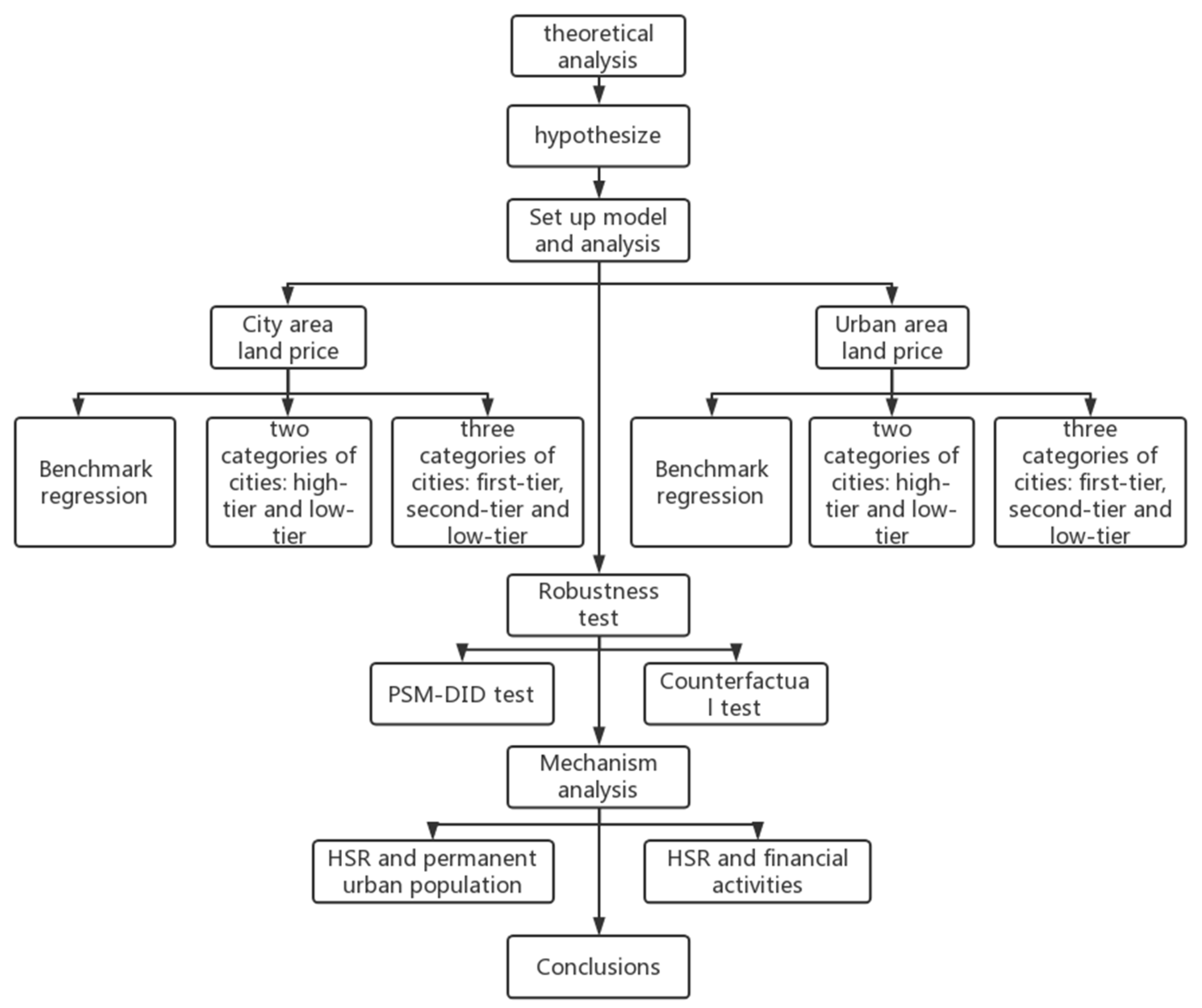
1. Introduction

Across the world, transport infrastructure is an important factor driving economic growth [1]. In 1964, Japan Shinkansen started a new era, HSR became a mode of transportation. In the 1990s, France, Germany, Spain, and other European countries built HSR on a large scale, and formed a European HSR network. Since then, the United States, South Korea, Turkey, and other countries have built HSR. Many scholars have studied how HSR affects economic development. Among them, the most remarkable is China’s HSR network construction. Since the opening of the Qin-Shenyang passenger dedicated line in October 2003, after nearly 20 years of development, the length of high-speed railways in China exceeded 40,000 km by the end of 2021, far exceeding the scale of other countries. When explaining the miracle of China’s economic growth, some people believe that China’s advanced transportation infrastructure construction is one of the important factors; so they have put forward policy suggestions for developing countries to build good transportation infrastructure first. Therefore, the study of the impact of China’s HSR on regional economy will provide reference significance for the construction of HSR around the world.

The HSR construction is one of the ongoing major strategic projects in China, and the economic development driven by HSR has become one of the hot spots. The uniqueness of HSR lies in its personnel transportation attribute, which accelerates the flow of personnel between the regions along the route; therefore, HSR brings more transmission of knowledge and information, as well as a series of communication derivative behaviors such as experiment, innovation, improvement, investment, and transaction. The advent of HSR reduces commuting time between regions, thus increasing regional accessibility [2], promoting regional and urban economic growth [3,4,5,6].

The economic growth of such regions and cities is structural, that is, it has different effects on different cities. In the future, as China’s HSR covers more regions and cities, the time and distance between cities will be compressed to a large extent. It is worthwhile to study the impact of the HSR on the regional economy, especially on the spatial pattern of China’s city economy. Many research have studied HSR from different theoretical and empirical perspectives. However, there are big divergences on whether the HSR promotes the balanced development of cities and regions or widens the gap. The study on the opening of HSR to promote cities and regional balance shows the spillover effect of central cities on surrounding cities along the line [7,8,9,10,11]. This effect expands the scope of the central area along the route [12,13,14].

Much of the existing literature shows that the opening of HSR does not balance cities and regional economic development [15,16]. In foreign countries, Pol P M J (2003) believes that the opening of HSR strengthens the rank of existing cities, and HSR strengthens the feature that the central city is an excellent area for knowledge and information exchange [17]. The opening of HSR in Spain and France drew similar conclusions [18]. The same phenomenon occurred in Japan and South Korea [9] because the siphon effect of HSR may accelerate the flow of investment factors into central cities [19]. In addition, the opening of HSR has improved the accessibility level of big cities [20], and delayed the speed of city economic convergence, so the regional gap is further widened [21]. This gap is achieved through investment activities [22,23], employment and salary [24], information transmission [25], allocation of financial elements [26,27,28], expanding market scope and labor force allocation [29], innovation activities [30], tourists and tourism activities [31,32], rising prices of residential land and commercial service facilities (hereinafter referred to as commercial land) [33], and it also shows the difference in housing prices [34,35].

Meanwhile, some literature has also studied the land use and transport interaction. Sands (1993) studied existing HSR, such as the Japanese Shinkansen, and the HSR in France and Germany, and found that land and property prices in cities rose due to the HSR opening [36]. Simmonds (2007) suggested that changes in transportation patterns have an impact on land use [37]. Hiroshi and Koichi (2018) found that after the opening of the HSR, the residential land prices in the Tokyo area increased significantly, indicating that the “space-time compression effect” of the HSR was capitalized in the land [38]. Deng and Wang (2018) using DID methods, founding that HSR causes city sprawl (ratio of the growth rate of city built-up area to that of population), especially large cities and cities in eastern China more affected by HSR [39]. Liu. et al. (2018) using DID methods, found the opening of the HSR significantly increased the real estate and land prices of the cities along the route [40].

The existing literature has few studies on land price and a lack of structural analysis of urban land price. Considering that city land price reflects the regional comprehensive competitiveness, a structural analysis of city land price in China is needed. The city construction land is divided into three types: industrial land, commercial use land, and residential land. As the main provider of construction land transfer, local governments have different logic for different types of land, which should be studied.

This paper believes that although the progress and application of modern communication technology reduces the cost of information collection and transmission, the location and spatial distance factors still exist for the “soft information” that mainly relies on the direct communication between people [28]. “Soft information” can include economic subject field research, environmental perception, communication, and practice verification. The progress of transportation can promote “face to face” contact, effectively reduce information asymmetry, and reduce the marginal cost of specific regional economic activities, which produce excess returns, attracting more market entity. The spatial distribution of stock economic entities and economic activities is unbalanced, and this excess return is also different in the spatial distribution. Moreover, the incremental economic entities tend to choose more advantageous areas, resulting in competition in specific locations manifested as land price (land rent). Therefore, the focus of this study is on the transfer price of residential and commercial use land before and after the opening of HSR, which reflects the impact of HSR on the economy of different cities and regions. Through this analysis, it can be seen whether the opening of HSR promotes the balanced development between cities.

The core of this paper is as follows: First, the opening of HSR has different effects on the economic activities of different cities. Moreover, economic activities make changes in the land supply and demand relationship. Second, commercial use land and residential land have different demand logic. Is there a difference in the impact of HSR opening on the two? Third, what is the impact of the opening of HSR on land prices divided into different areas of the city? (considered as city area and urban area: city area refers to the whole administrative divisions of a city, including urban area, county and township parts; urban area refers to the main city of a city, mainly divided into districts)

The subsequent arrangement is as follows (as Figure 1 shows): Section 2 is the theoretical analysis and the research assumptions; Section 3 is the model setting and data description; Section 4 reports the empirical results; Section 5 is the robustness test; Section 6 is the mechanism analysis; and Section 7, are the research conclusions.

2. Theoretical Analysis and Research Hypothesis

2.1. Mathematical Model

2.1.1. Land Supply—The Government Behavior

For local government, land transfer income is a core part of the budget income of government-managed funds, and the freest part of the fiscal “four books”. Local governments have the incentive to increase this part of revenue. At present, land transfer is mainly supplied by local government to the market by means of “bidding, auction and hanging”, so we can regard local government as the monopoly party of land supply. At the same time, given that local governments have another source of “disposable income” by injecting land into city investment companies that lend to financial institutions for urban construction funds, local governments also have an incentive to push land prices higher.

2.1.2. Land Demand—Equilibrium Solution for the Market

The market demand for urban land can be regarded as the “recognition” of the market to the city economic development prospects. Under the competition mechanism of “bidding, auction and hanging”, local governments, as the monopoly of land supply, obtain consumer surplus as much as possible. Therefore, the market demand for land is the main variable affecting the land price.

The basis of the micro mechanism of this paper is that exogenous HSR variables bring excess returns to specific regions (cities), which causes the land competition of market subjects for specific regions. Therefore, land factor demand variables should be added to the current model.

With the following considerations: first, the producer market is competitive and there is no excess profit, so the excess return of HSR opening is expressed by regional land rent. Second, cities have economies of scale because of the existence of agglomeration economy, and the different effects of the opening of HSR can be seen. Third, as the producer perspective and consumer behavior, there is the influence of HSR opening on urban land price in equilibrium.

In view of the above considerations, this paper is based on the basic model of Fujita and Paul Krugman (2001) [41], and adds the land element variables. See Appendix B for detailed procedures.

2.2. Assumptions Proposed

For a city, HSR can improve its accessibility level, reduce transportation costs, and generate geographical aggregation under the condition of increasing remuneration for scale. For a single enterprise, sharing, learning, matching, and other functions that bring additional benefits attract enterprises, but also to bring more employment and population. In the case of a limited city land space, more individuals and enterprises [14], lead to land demand (location demand). According to the land competitive rent theory (also, 1962), the competition for an exclusive location increases the land price, and the aggregate rent is manifested through the land price (location price). Within the city, the agglomeration degree is higher, and is manifested in Formula (A1) in Appendix B, the production efficiency r is higher. Hypothesis 1 is therefore proposed.

$$\frac{\partial \left(-a\right)}{\partial r}>0$$

Hypothesis 1 (H1):

HSR opening increases land prices in cities, especially in urban areas.

Compared with ordinary railways, HSR passengers have stronger business attributes, passengers are mostly middle and high managers of enterprises, and master a large number of non-standardized and subjective cognition of “soft information” [25]. HSR provides “face to face” communication convenience and promotes the realization of economic benefits. Because big cities have a larger economy, more population and richer market segments, their information can be better used. As shown in Formula (A1) in Appendix B, the connected market range R is larger. Hypothesis 2 is thus proposed.

$$\frac{\partial \left(-a\right)}{\partial R}>0$$

Hypothesis 2 (H2):

The opening of HSR has a greater impact on land prices in high-tier cities.

Local government is the absolute monopoly in the primary land market. The economic benefits of land transfer are divided into direct land transfer income and taxes based on economic activities on the land. After the transfer and development of residential land, residents living there make no direct tax revenue, while after the sale of commercial use land, there is continuous economic activity and taxes. So, for local governments, the transfer of residential land is mainly a single income; therefore, the transfer behavior of residential land is to sell as high a price as possible, while the transfer of commercial land should consider that high land price is not conducive to investment and other adverse factors. Thus, we propose Hypothesis 3.

Hypothesis 3 (H3):

In comparison, the impact of HSR opening on residential land prices is higher than that of commercial land prices.

3. Measurement Model, Variable Selection and Data Processing

3.1. Model Setting

The impact of HSR opening on the regional economy is a “quasi-natural experiment”. Most studies have used the DID method to measure the effect of HSR opening, and this paper will also use the DID method. The basic idea is to take the price of commercial land and residential land (divided into urban and urban areas, respectively) as the explanatory variables, and the HSR opening as the core explanatory variable, and other control variables are added.

In this paper, cities with HSR from 2011 to 2018 are used as the processing group, and cities without HSR are used as the control group, thus obtaining the impact of the quasi-natural experiment of HSR on the land price. At the same time, this paper focuses on the impact of HSR opening on heterogeneous cities, so the city level virtual variables are added. Considering the possible time delay of the economic effect of HSR opening, the situation from the opening year to 5 years after opening was studied, respectively. The basic model is as follows:

Y_it = β_i + β_t + (β₂ + α * L) * HSR_it + β * X_it + e_it

where Y_it is the land price of city i in year t. β_t is the city fixed effect and the year fixed effect. L is a dummy variable that represents the city level (see below). X_it is the control variable. HSR_it is a dummy variable, if city i passes HSR in year t, and the value is 1, otherwise 0, so the lag effect of HSR opening is similar. The variable HSR_it estimated coefficient of the β₂ which is the focus of this study: if β₂ > 0, shows that the opening of the HSR affects the land price, and the specific numerical meaning of the coefficient is the impact of the HSR opening on the land price growth; according to theory and hypothesis, if α is not 0, it shows that the opening of HSR has different effects on land prices in different types of cities.

3.2. Variable Selection

• Dependent variables

There are four categories of explained variables in this paper: city area commercial use land price, city area residential land price, urban area commercial use land price, and urban area residential land price. These four variables involve two dimensions: one is the characteristic land use, namely, divided into commercial industry and residential housing; the other is land location, divided into city area and urban area (city area refers to the whole administrative divisions of a city, including urban area, county and township parts; urban area refers to the main city of a city, mainly divided into districts). The purpose of this division is to see the impact of the opening of HSR on the land prices of different characteristics and locations to enrich the research conclusions.

2.

Core variable

The first dummy variable HSR is whether HSR is open. Similar to other research literature, the variable value is 1 and 0. The opening of HSR is reflected in the establishment of stations within prefecture-level cities and realizing passenger traffic. If it is realized before 30 June, it is counted as the same year, otherwise it is included in the next year. For the cities that have opened a number of HSR lines, this paper mainly focuses on the earliest opening of the HSR.

The second dummy variable is the city level. In this paper, all the sample cities are divided into first-tier cities (including new first-tier cities), second-tier cities, and low-tier cities to test the impact of HSR opening on land prices in different levels of cities. City level is according to the China Business News New First-tier City Research Institute released list. Considering only four first-tier cities as a sample is too small, we added new first-tier cities from the 2013–2018 lists, so there are 21 first-tier cities and 27 s-tier cities. For the convenience of narration, this paper calls the first-tier and second-tier cities as high-tier cities (the geographical location of the cities are shown as Figure A1 in Appendix A), while the rest of the cities are low-tier cities.

3.

Control variable

On the basis of reference to previous literature, the control variables were selected as follows (as shown in the

Table 1. Selection significance of each variable.

	Variable	Symbol	Select the Significance of This Variable
Explained variable	City area commercial use land price	lny1	Growth rate of city area commercial use land transfer price
	City area residential land price	lny2	Growth rate of city area residential land transfer price
	Urban area commercial use land prices	lny3	Growth rate of urban area commercial use land transfer price
	Urban area residential land prices	lny4	Growth rate of urban area residential land transfer price
Explanatory variable	The year of the opening of the HSR	HSR0	The impact of HSR opening as the explanatory variable on land prices is observed through the current period and the lag period.
	One year after the HSR was opened	HSR
	2 years after the HSR was opened	HSR2
	3 years after the HSR was opened	HSR3
	4 years after the HSR was opened	HSR4
	5 years after the HSR was opened	HSR5
Dummy variable	First-tier cities (including new first-tier cities)	LU	It is used to distinguish the impact of the opening of HSR on cities at different levels and reflect the structural effect of HSR. 21 first-tier cities: Beijing, Tianjin, Chongqing, Shanghai, Zhengzhou, city, Changsha, Wuhan, city, Shenzhen, Shenzhen, Dongguan, Chengdu, Qingdao, Hangzhou, nanbo, Xiamen, Nanjing, Wuxi, Suzhou, Shenyang, Dalian, and Xi’an. 27 s-tier cities: Shijiazhuang, Baoding, Foshan, Huizhou, Zhongshan, Nanning, Taiyuan, Jinan, Yantai, Weifang, Lanzhou, Guiyang, Kunming, Nanchang, Wenzhou, Shaoxing, Jiaxing, Jinhua, Taizhou, Fuzhou, Quanzhou, Xuzhou, Changzhou, Nantong, Hefei, Harbin, and Changchun. 48 high-tier cities: 21 first-tier and 27 s-tier cities.
	Second-tier city	LM
	High-tier city	LH
Controlled variable	GDP growth rate (%)	gdpg	For people and market entities, economic growth means more opportunities for participation and development space, so a city’s economic growth attracts population and market entities to gather, thus affecting land prices.
	The proportion of tertiary industry (%)	tert	The tertiary industry is the main part of employment, but also the embodiment of commercial agglomeration, affecting the price of residential and commercial land.
	Total retail sales of consumer goods	lncons	Reflects the degree of commercial development of the city.
	Per capita disposable income of urban households	lnincome	Income has an impact on population mobility, leading to population clusters and thus affecting land prices.
	Urban resident population	lnupop	Population aggregation has a significant impact on land prices.
	Number of primary and secondary schools	lnschl	Reflects the level of urban public services and affects the population flow.
	Number of beds in health institutions	lnhosl

): GDP growth (gdpg), tertiary industry proportion (tert), total retail sales of consumer goods (cons), per capita disposable income of urban households (income), urban permanent population (upop), number of primary and secondary schools (schl), and number of beds in health institutions (hosl). Among them, GDP growth means the market increment of high growth cities is more attractive to potential market entities. The per capita disposable income is the main factor to attract population flow in. The third industry development, total retail sales of consumer goods, and urban population direct demand for urban commercial and residential land. The number of primary and secondary schools and hospital beds reflects the city’s public service supply level.

3.3. Data Source and Processing

Considering the availability of data and the opening time of HSR, this paper studied the municipalities and prefecture-level cities from 2011 to 2018. Due to the availability of land transfer data, 223 cities were left (according to the previous definition, 48 high-tier cities, and 175 low-tier cities). Land prices, total retail sales of consumer goods, per capita disposable income, permanent urban population, the number of primary and secondary schools, and the number of beds in health institutions were treated logarithmically. The land price data come from Guosen Real Estate Information Network—macroeconomic and real estate database. This paper added up the land transfer amount of each city and weighted average according to the area, and found the unit price of the land transfer price in the current year. The economic data of prefecture-level cities come from the statistical yearbooks and statistical bulletins of various provinces and prefecture-level cities. Descriptive statistics for each variable are shown in

Table 2. The descriptive statistics for each variable.

Variable	Symbol	Sample Number	Mean	Standard Deviation	Min Value	Max Value
City area commercial use of land price	lny1	1784	3.1849	0.3730	1.3802	5.2122
City area residential land price	lny2	1784	3.3495	0.3668	2.2529	5.0236
Urban area commercial use of land prices	lny3	1784	3.2962	0.3912	1.9956	5.2122
Urban area residential land prices	lny4	1784	3.4514	0.3801	2.2625	5.0236
GDP growth rate	gdpg	1784	9.0742	3.4218	−14.20	49.2791
The proportion of tertiary industry	tert	1784	40.5665	9.3838	14.3632	80.9817
Total retail sales of consumer goods	lncons	1784	2.8380	0.4175	1.7456	4.1529
Per capita disposable income of urban households	lnincome	1784	4.4386	0.1362	4.0519	4.9336
Urban resident population	lnupop	1784	2.3431	0.3037	1.5490	3.3490
Number of primary and secondary schools	lnschl	1784	2.8673	0.3120	1.9031	3.8134
Number of beds in health institutions	lnhosl	1784	4.2973	0.2950	2.9053	5.3145
The year of the HSR opening	HSR0	1784	0.4916	0.5001	0	1
1 year after the HSR was opened	HSR1	1784	0.4238	0.4943	0	1
2 years after the HSR was opened	HSR2	1784	0.3492	0.4769	0	1
3 years after the HSR was opened	HSR3	1784	0.2702	0.4442	0	1
4 years after the HSR was opened	HSR4	1784	0.1962	0.3972	0	1
5 years after the HSR was opened	HSR5	1784	0.1396	0.3466	0	1
First-tier cities (including new first-tierones)	LU	1784	0.0942	0.2921	0	1
Second-tier city	LM	1784	0.1211	0.3263	0	1
High-tier city	LH	1784	0.2152	0.4111	0	1

.

4. Analysis of the Empirical Results

4.1. City Area:Regression Analysis of Commercial Use and Residential Land Prices

4.1.1. Benchmark Regression

This section mainly studies the overall impact of HSR opening on the price of commercial use and residential land in the city area, and the results are shown in

Table 3. Overall impact of HSR opening on city area commercial and residential land prices.

	Impact on City Area Commercial Use Land Price (lny1)		Impact on the City Area Residential Land Price (lny2)
	(1)	(2)	(3)	(4)
HSR0	0.0074 (0.36)	0.0075 (0.37)	0.0053 (0.33)	0.0066 (0.42)
HSR1	0.0171 (0.89)	0.0177 (0.92)	0.0209 (1.25)	0.0181 (1.14)
HSR2	−0.0159 (−0.91)	−0.0162 (−0.92)	0.0425 *** (2.69)	0.0379 ** (2.53)
HSR3	0.0069 (0.39)	0.0068 (0.39)	0.0639 *** (4.00)	0.0559 *** (3.68)
HSR4	0.0138 (0.70)	0.0162 (0.83)	0.0771 *** (4.37)	0.0702 *** (4.10)
HSR5	0.0160 (0.75)	0.0175 (0.81)	0.0787 *** (3.94)	0.0718 *** (3.66)
controlled variable	not have	have	not have	have

Note: *** represents the significance level of 1%, ** represents 5%, with t value in parentheses.

. It can be seen the opening of HSR has no significant impact on the price of city area commercial use land within 5 years, and impacts mainly residential land, which verifies Hypothesis 3.

From columns (3) and (4), 2 years after the opening of HSR there is a positive impact on the residential land price in the city area. Compared with the cities without HSR, the residential land price in the opening cities increased by 3.79%, 5.59%, 7.02%, and 7.18%, respectively. The regression coefficient shows that the opening of HSR increases the land prices of cities and shows a trend of increasing year by year.

4.1.2. Regression Results of Two Categories of Cities: High-Tier and Low-Tier

We first divided 223 cities into two categories: 48 high-tier cities (first-tier and second-tier cities) and 175 low-tier cities. For the variables L_H as dummy variables, the high-tier city value is 1 and the rest are 0, and the regression results are shown in

Table 4. City Level Model 1: Impact of HSR opening on the price of commercial use and residential land in the city area.

	Impact on City Area Commercial Use Land Price (lny1)		Impact on City Area Residential Land Price (lny2)
	(5)	(6)	(7)	(8)
HSR0	0.0062 (0.29)	0.0068 (0.33)	−0.0159 (−0.96)	−0.0126 (−0.79)
HSR1	0.0115 (0.58)	0.0129 (0.66)	−0.0049 (−0.28)	−0.0043 (−0.27)
HSR2	−0.0128 (−0.65)	−0.0118 (−0.60)	0.0183 (1.07)	0.0184 (1.11)
HSR3	0.0177 (0.93)	0.0182 (0.96)	0.0285 * (1.74)	0.0255 * (1.61)
HSR4	0.0126 (0.55)	0.0167 (0.72)	0.0347 * (1.80)	0.0340 * (1.80)
HSR5	0.0111 (0.41)	0.0143 (0.51)	0.0275 (1.19)	0.0270 (1.17)
HSR0 × LH	0.0076 (0.12)	0.0046 (0.08)	0.1354 *** (3.01)	0.1220 *** (2.79)
HSR1 × LH	0.0271 (0.55)	0.0237 (0.50)	0.1250 *** (3.35)	0.1108 *** (3.08)
HSR2 × LH	−0.0118 (−0.32)	−0.0168 (−0.48)	0.0909 *** (2.77)	0.0757 *** (2.39)
HSR3 × LH	−0.0319 (−0.91)	−0.0348 (−1.02)	0.1043 *** (3.21)	0.0926 *** (2.89)
HSR4 × LH	0.0028 (0.08)	−0.0012 (−0.03)	0.0994 *** (3.13)	0.0872 *** (2.76)
HSR5 × LH	0.0098 (0.27)	0.0065 (0.18)	0.1033 *** (3.05)	0.0921 *** (2.67)
Controlled variable	Not have	Have	Not have	Have

Note: *** represents the significance level of 1%, * represents 10%, with t value in parentheses.

. The results show that the opening of HSR has no significant impact on the price of city area commercial use land, while the impact is mainly on the price of city area residential land.

From columns (7) and (8), the positive impact of the opening of HSR on residential land prices is concentrated in high-tier cities. From the opening year to 5 years after, the coefficient of city grade dummy variables L is positive. According to the coefficient of the opening of HSR, from the opening year to 2 years after opening, the price of residential land in high-tier cities increased by 12.2%, 11.1%, and 7.57%, while it did not impact low-tier cities. The price of residential land in low-tier cities increased by 2.55% and 3.4% at the 3rd and 4th years after the opening. Five years after the opening of HSR, the price of residential land in low-tier cities did not increase significantly, high-tier cities still have “HSR dividend”.

Compared with the results of the previous benchmark regression, it can be seen that the positive impact of the opening of HSR on city area land prices is mainly concentrated in high-tier cities, which verifies Hypothesis 2. Moreover, the residential land prices in high-tier cities are not only reflected in the year of opening, and the impact lasts longer.

4.1.3. Regression Results of Three Categories of Cities: First-Tier, Second-Tier, and Low-Tier Cities

This section continues to subdivide the high-tier cities into first-tier (including new first-tier, the same below) cities (dummy variables L_U), second-tier cities (dummy variable L_M), and low-tier cities, the regression results are shown in

Table 5. City Grade Model 2: Impact of HSR opening on the price of commercial use and residential land in the city area.

	Impact on City Area Commercial Use Land Price (lny1)		Impact on City Area Residential Land Price (lny2)
	(9)	(10)	(11)	(12)
HSR0	0.0063 (0.30)	0.0068 (0.33)	−0.0159 (−0.96)	−0.0126 (−0.79)
HSR1	0.0117 (0.59)	0.0130 (0.66)	−0.0048 (−0.28)	−0.0043 (−0.27)
HSR2	−0.0127 (−0.64)	−0.0118 (−0.60)	0.0182 (1.06)	0.0183 (1.11)
HSR3	0.0178 (0.93)	0.0182 (0.96)	0.0283 * (1.73)	0.0254 * (1.61)
HSR4	0.0126 (0.55)	0.0166 (0.72)	0.0347 * (1.80)	0.0342 * (1.80)
HSR5	0.0111 (0.41)	0.0143 (0.51)	0.0275 (1.19)	0.0270 (1.17)
HSR0 × LU	−0.1216 (−1.27)	−0.1156 (−1.23)	0.1204 (1.19)	0.1137 (1.27)
HSR1 × LU	−0.0702 (−1.13)	−0.0658 (−1.07)	0.1175 (1.56)	0.1036 (1.51)
HSR2 × LU	−0.0481 (−0.92)	−0.0481 (−0.93)	0.1275 *** (2.82)	0.1104 *** (2.70)
HSR3 × LU	−0.0435 (−0.92)	−0.0428 (−0.91)	0.1560 *** (3.85)	0.1429 *** (3.57)
HSR4 × LU	−0.0131 (−0.29)	−0.0146 (−0.33)	0.1501 *** (3.82)	0.1363 *** (3.46)
HSR5 × LU	0.0189 (0.41)	0.0174 (0.37)	0.1414 *** (3.38)	0.1277 *** (2.98)
HSR0 × LM	0.0476 (0.68)	0.0419 (0.62)	0.1400 *** (2.91)	0.1246 ** (2.55)
HSR1 × LM	0.0753 (1.26)	0.0678 (1.17)	0.1287 *** (3.35)	0.1144 *** (2.97)
HSR2 × LM	0.0155 (0.34)	0.0065 (0.15)	0.0635 (1.50)	0.0497 (1.18)
HSR3 × LM	−0.0205 (−0.44)	−0.0270 (−0.59)	0.0536 (1.23)	0.0440 (1.02)
HSR4 × LM	0.0212 (0.47)	0.0142 (0.31)	0.0405 (1.94)	0.0311 (0.80)
HSR5 × LM	−0.0013 (−0.33)	−0.0062 (−0.14)	0.0570 (1.41)	0.0501 (1.23)
Controlled variable	Not have	Have	Not have	Have

Note: *** represents the significance level of 1%, ** represents 5%, * represents 10%, with t value in parentheses.

. Similarly, the opening of HSR has no significant impact on the price of city area commercial use land, mainly on the price of city area residential land.

For low-tier cities, the impact of the HSR opening on city area is that residential land prices increased by 2.54% and 3.42% at the 3rd and 4th years after the opening, respectively.

After dividing high-tier cities into first-tier and second-tier cities, the opening of HSR has a positive impact on city area residential land prices in second-tier cities at first, it increased by 12.5% and 11.4% in the opening year and 1 year after, respectively. At this time, no effect on first-tier cities was found. At 2 years after the opening, the impact on the second-tier cities was not obvious, but the first-tier cities began to be affected by HSR opening; the influence effect continues to 5 years after the opening. Residential land price rose more than 10%, especially opening after 3rd and 4th years, HSR on first-tier city area residential land price effect increased by 16.8% and 17.1%, which verifies Hypothesis 2.

Based on the comprehensive regression analysis conclusion above, HSR opening has obvious positive effects on residential land prices. Among them, the high-tier (second-tier and first--tier) cities’ residential land price rises are more obvious, are influenced by HSR longer, and start earlier; thus widening the gap between the cities.

In the high-tier cities sample, the opening of HSR first has an impact on the rise of residential land prices in second-tier cities. However, 2 years after the opening, it begins to have a positive impact on first-tier cities and continues, which verifies Hypotheses 2 and 3. This shows that the opening of HSR has widened the economic gap between cities, which is reflected in the cities with HSR and non-HSR, but also shows the trend of “the strong are stronger”.

4.2. Urban Area:Regression Analysis of Commercial Use and Residential Land Prices

This section mainly studies the relationship between the price of urban area commercial use and residential land and the opening of HSR. First is the overall regression results analysis, followed by the city-grade regression results analysis.

4.2.1. Benchmark Regression

Taking the urban area as the research object, regardless of urban grade, as

Table 6. Overall impact of HSR opening on urban area commercial and residential land prices.

	Impact on Urban Area Commercial Use Land Price (lny3)		Impact on Urban Area Residential Land Price (lny4)
	(13)	(14)	(15)	(16)
HSR0	0.0042 (0.17)	0.0046 (0.19)	0.0048 (0.24)	0.0069 (0.35)
HSR1	0.0023 (0.09)	0.0024 (0.10)	0.0199 (1.10)	0.0172 (0.98)
HSR2	−0.0167 (−0.73)	−0.0175 (−0.76)	0.0441 ** (2.52)	0.0384 ** (2.27)
HSR3	−0.0237 (−1.02)	−0.0260 (−1.13)	0.0651 *** (3.69)	0.0554 *** (3.25)
HSR4	−0.0057 (−0.23)	−0.0070 (−0.29)	0.0768 *** (4.02)	0.0674 *** (3.62)
HSR5	0.0247 (0.96)	0.0234 (0.91)	0.0772 *** (3.76)	0.0687 *** (3.38)
Controlled variable	Not have	Have	Not have	Have

Note: *** represents the significance level of 1%, ** represents 5%, with t value in parentheses.

shows, the impact of HSR opening on the price of urban area commercial use land is not significant, but it has a significant impact on the residential land price 2 years after the opening.

Two years after the opening of the HSR, the price of urban area residential land increased by 3.84%, 5.54%, 6.74%, and 6.87%. At the same time, the impact of HSR opening has a time delay on the urban area residential land price, and it has a positive impact. The influence coefficient gradually increases with time. In addition, compared with the data in Table 3, the difference coefficient of the HSR opening on urban area land price is not obvious compared with the city area.

4.2.2. Regression Results of Two Categories of Cities: High-Tier and Low-Tier

Compared with the city area, the opening of HSR has a positive impact on the price of commercial use land in urban areas. As

Table 7. City Level Model 1: Impact of HSR opening on the price of commercial use and residential land in the urban area.

	Impact on Urban Area Commercial Use Land Price (lny3)		Impact on Urban Area Residential Land Price (lny4)
	(17)	(18)	(19)	(20)
HSR0	−0.0032 (−0.12)	−0.0035 (−0.14)	−0.0198 (−0.94)	−0.0158 (−0.77)
HSR1	−0.0133 (−0.48)	−0.0140 (−0.50)	−0.0092 (−0.49)	−0.0090 (−0.49)
HSR2	−0.0276 (−1.03)	−0.0288 (−1.07)	0.0139 (0.69)	0.0122 (0.62)
HSR3	−0.0244 (−0.92)	−0.0276 (−1.05)	0.0355 * (1.88)	0.0298 (1.62)
HSR4	−0.0180 (−0.59)	−0.0196 (−0.64)	0.0444 ** (2.08)	0.0395 * (1.88)
HSR5	0.0206 (0.58)	0.0186 (0.52)	0.0487 ** (2.02)	0.0454 * (1.87)
HSR0 × LH	0.0470 (0.73)	0.0515 (0.81)	0.1567 *** (3.79)	0.1439 *** (3.60)
HSR1 × LH	0.0754 (1.51)	0.0810 * (1.65)	0.1411 *** (4.00)	0.1292 *** (3.77)
HSR2 × LH	0.0409 (1.00)	0.0439 (1.11)	0.1137 *** (3.48)	0.1014 *** (3.22)
HSR3 × LH	0.0021 (0.05)	0.0050 (0.12)	0.0869 ** (2.49)	0.0781 ** (2.23)
HSR4 × LH	0.0289 (0.67)	0.0306 (0.72)	0.0759 ** (2.24)	0.0672 *** (1.97)
HSR5 × LH	0.0082 (0.19)	0.0099 (0.23)	0.0574 (1.62)	0.0479 (1.32)
Controlled variable	Not have	Have	Not have	Have

Note: *** represents the significance level of 1%, ** represents 5%, * represents 10%, with t value in parentheses.

shows, one year after the opening, the price of commercial use land in high-tier cities increased by 8.1%, but there is an insignificant impact on low-tier cities.

Relatively, the impact of HSR on urban area residential land prices is more obvious; by column (20), HSR made the high-tier city urban area residential land prices rise 14.39%, by the 5th year after the opening. In high-tier cities, compared with the city area residential land price coefficient, the impact coefficient on urban areas is about 2–3% higher within 3 years after opening, which verifies Hypothesis 1.

In addition, in terms of low-tier cities, the coefficient of HSR opening impact on urban area residential land prices is higher than on city area ones. Therefore, for low-tier cities, the opening of HSR mainly affects the price of urban area residential land, which also verifies Hypothesis 1.

4.2.3. Regression Results of Three Categories of Cities: First-Tier, Second-Tier, and Low-Tier Cities

The high-tier cities were divided into first-tier and second-tier cities. At the same time, comparison of the urban area results and the city area results have the following conclusions.

First, in terms of the price of commercial use land, the opening of HSR mainly affects second-tier cities. As

Table 8. City Grade Model 2. The impact of HSR opening on the price of commercial and residential land in urban areas.

	Impact on Urban Area Commercial Use Land Price (lny3)		Impact on Urban Area Residential Land Price (lny4)
	(21)	(22)	(23)	(24)
HSR0	−0.0031 (−0.12)	−0.0035 (−0.14)	−0.0197 (−0.94)	−0.0158 (−0.77)
HSR1	−0.0131 (−0.47)	−0.0140 (−0.50)	−0.0092 (−0.49)	−0.0090 (−0.49)
HSR2	−0.0274 (−1.02)	−0.0288 (−1.07)	0.0138 (0.69)	0.0122 (0.62)
HSR3	−0.0243 (−0.92)	−0.0276 (−1.05)	0.0353 * (1.87)	0.0297 (1.61)
HSR4	−0.0180 (−0.59)	−0.0197 (−0.65)	0.0444 ** (2.08)	0.0397 * (1.89)
HSR5	0.0206 (0.58)	0.0186 (0.52)	0.0487 ** (2.02)	0.0454 * (1.87)
HSR0 × LU	−0.0525 (−0.78)	−0.0431 (−0.68)	0.1425 * (1.70)	0.1295 ** (1.77)
HSR1 × LU	0.0008 (0.02)	0.0122 (0.25)	0.1430 ** (2.19)	0.1287 ** (2.24)
HSR2 × LU	0.0043 (0.08)	0.0097 (0.19)	0.1418 *** (3.19)	0.1256 *** (3.21)
HSR3 × LU	−0.0235 (−0.44)	−0.0187 (−0.36)	0.1347 *** (3.21)	0.1235 *** (3.01)
HSR4 × LU	−0.0007 (−0.01)	0.0029 (0.06)	0.1224 *** (3.13)	0.1122 *** (2.88)
HSR5 × LU	0.0042 (0.08)	0.0076 (0.15)	0.1028 ** (2.50)	0.0911 ** (2.14)
HSR0 × LM	0.0778 (1.00)	0.0807 (1.05)	0.1611 *** (3.57)	0.1483 *** (3.31)
HSR1 × LM	0.1123 * (1.76)	0.1149 * (1.82)	0.1401 *** (3.69)	0.1295 *** (3.36)
HSR2 × LM	0.0683 (1.36)	0.0694 (1.39)	0.0925 ** (2.28)	0.0834 ** (2.06)
HSR3 × LM	0.0272 (0.47)	0.0280 (0.49)	0.0402 (0.82)	0.0341 (0.70)
HSR4 × LM	0.0633 (1.10)	0.0623 (1.08)	0.0221 (0.48)	0.0156 (0.34)
HSR5 × LM	−0.0165 (0.24)	0.0126 (0.23)	0.0023 (0.05)	−0.0028 (−0.06)
Controlled variable	Not have	Have	Not have	Have

Note: *** represents the significance level of 1%, ** represents 5%, * represents 10%, with t value in parentheses.

shows, one year after the opening, the price of commercial use land increased by 11.5% in second-tier cities (8.1% in high-tier cities). According to the above analysis, HSR has no impact on city area commercial use land price.

Second, the opening of HSR affects the price of urban area residential land in first-tier cities the most obviously, which verifies Hypothesis 1 and 2. On the one hand, it lasts longer and positively affects the residential land price in first-tier cities from the opening year, while impacting the city area from the 2nd year after opening. On the other hand, compared with the data in Table 5, the influence coefficient on the urban area residential land price in first-tier cities exceeds the impact on city areas. This shows that during the following 3 years of the opening, it mainly affected urban area residential land in first-tier cities, and then caused “diffusion” within the city area, making the suburban land price begin to rise.

Third, for the residential land prices in second-tier cities, the opening of HSR has a more significant impact on urban areas, which verifies Hypothesis 1. On the one hand, the positive effect of HSR opening on the urban area residential land price lasted 3 years, while the impact on the city area lasted 2 years. On the other hand, compared with the data in Table 5, the influence coefficient of the urban area residential land price in second-tier cities is higher than the city area in the first 3 years (the urban area value was 14.8%, 12.95%, and 8.34% respectively, while the city area value was 12.5% and 11.4%). This shows that for the residential land prices in second-tier cities, the opening of HSR is more favorable for urban areas. Second-tier cities do not have a municipal “diffusion” effect as in first-tier cities.

To sum, the opening of HSR first affects the urban area residential land price in first-tier cities, and then the second-tier cities. After that, it impacts on the city area land price in second-tier and above cities (mainly non-urban), showing an obvious polarization effect.

5. Robustness Test

5.1. PSM-DID Test

The assumption of DID is that the city time effect of the experimental group and the control group are consistent, and the choice of the treatment group is random, which means the construction of HSR is a natural experiment, and the city itself cannot affect the decision of HSR construction. However, in the decision-making process of constructing HSR, such as the priority formation of transportation network between big cities, the starting point of this paper is heterogeneous cities, so the assumption of DID is violated. To verify the robustness of the conclusions, the score tendency matching method (PSM) method is needed.

The basic idea is: Build a city that has similar characteristics to a city before HSR opened, as a control group. The only difference should be “through HSR”; compare the two types of cities in the case of HSR opening land price change, and obtain the relationship between HSR opening and land price. First, use the PSM to find the matching group; then use the matched processing group and the control group to make the DID estimation, the corresponding regression equation is as follows:

Y_it^PSM = β_i + β_t + β₂ * HSR_it + α * L * HSR_it + β * X_it + e_it

After matching, regression was performed according to two and three city rank patterns in the previous paragraph, and the results are shown in

Table 9. Regression coefficients of cities into high and low lines under the P S M-DID method.

	Impact on City Area Commercial Use Land Price (lny1)	Impact on City Area Residential Land Price (lny2)	Impact on Urban Area Commercial Use Land Price (lny3)	Impact on Urban Area Residential Land Price (lny4)
HSR0	−0.0166 (−0.70)	−0.0514 (−0.38)	−0.0121 (−0.43)	−0.0153 (−0.64)
HSR1	0.0218 (0.93)	−0.0060 (−0.67)	0.0047 (0.14)	−0.0197 (−0.83)
HSR2	−0.0243 (−0.96)	−0.0060 (−0.27)	−0.0452 (−1.26)	0.0028 (0.10)
HSR3	−0.0145 (−0.52)	−0.0070 (−0.37)	−0.0756 ** (−2.14)	−0.0022 (−0.10)
HSR4	0.0167 (0.46)	0.0184 (0.72)	−0.0354 (−0.79)	−0.0018 (−0.08)
HSR5	0.0415 (1.08)	−0.0264 (−0.83)	0.0573 (1.11)	0.0254 (0.75)
HSR0 × LH	0.0246 (0.39)	0.0850 (2.24)	0.0751 (1.09)	0.1308 *** (3.12)
HSR1 × LH	0.0112 (0.22)	0.0931 *** (2.42)	0.0856 (1.49)	0.1221 *** (3.16)
HSR2 × LH	−0.0130 (−0.34)	0.0670 ** (1.89)	0.0500 (1.08)	0.0697 * (1.88)
HSR3 × LH	0.0065 (0.16)	0.0889 *** (2.61)	0.0502 (0.96)	0.0528 * (1.36)
HSR4 × LH	0.0399 (0.93)	0.0699 ** (2.03)	0.0501 (1.01)	0.0716 * (1.76)
HSR5 × LH	−0.0051 (−0.12)	0.1052 *** (2.72)	−0.0433 (−0.84)	0.00258 (0.60)
Controlled variable	Have	Have	Have	Have

Note: *** represents the significance level of 1%, ** represents 5%, * represents 10%, with t value in parentheses.

and

Table 10. Regression coefficients of cities classified as first-tier, second-line, and low-line cities under the P S M-DID method.

	Impact on City Area Commercial Use Land Price (lny1)	Impact on City Area Residential Land Price (lny2)	Impact on Urban Area Commercial Use Land Price (lny3)	Impact on Urban Area Residential Land Price (lny4)
HSR0	−0.0164 (−0.69)	−0.0514 (−0.38)	−0.0119 (−0.42)	−0.0153 (−0.64)
HSR1	0.0216 (0.92)	−0.0141 (−0.67)	0.0046 (0.14)	−0.0198 (−0.83)
HSR2	−0.0247 (−0.98)	−0.0055 (−0.85)	−0.0457 (−1.27)	0.0031 (0.12)
HSR3	−0.0147 (−0.53)	−0.0068 (−0.36)	−0.0758 ** (−2.14)	−0.0020 (−0.09)
HSR4	0.0166 (0.46)	0.0199 (0.79)	−0.0355 (−0.78)	−0.0015 (−0.06)
HSR5	0.0412 (1.07)	−0.0272 (−0.85)	0.0572 (1.11)	0.0259 (0.76)
HSR0 × LU	−0.0907 (−0.84)	0.1042 (1.22)	−0.0231 (−0.32)	0.1342 ** (1.65)
HSR1 × LU	−0.0949 (−1.51)	0.0797 (1.11)	0.0028 (0.05)	0.1080 ** (1.70)
HSR2 × LU	−0.0448 (−0.81)	0.0976 ** (2.25)	0.0172 (0.30)	0.0914 ** (1.97)
HSR3 × LU	−0.0187 (−0.34)	0.1251 *** (3.14)	0.0104 (0.16)	0.0842 ** (1.95)
HSR4 × LU	0.0366 (0.77)	0.1244 *** (2.86)	0.0476 (0.87)	0.0996 ** (2.07)
HSR5 × LU	0.0092 (0.18)	0.1383 *** (2.91)	−0.0396 (−0.68)	0.0524 ** (1.65)
HSR0 × LM	0.0595 (0.85)	0.0745 (1.96)	0.1048 (1.26)	0.1298 *** (2.82)
HSR1 × LM	0.0645 (1.06)	0.0998 ** (2.55)	0.1271 * (1.77)	0.1292 *** (3.12)
HSR2 × LM	0.0146 (0.32)	0.0403 (0.86)	0.0785 (1.37)	0.0507 (1.11)
HSR3 × LM	0.0316 (0.66)	0.0528 (1.05)	0.09 (1.29)	0.0215 (0.37)
HSR4 × LM	0.0438 (0.76)	0.0052 (0.14)	0.0531 (0.83)	0.0334 (0.60)
HSR5 × LM	−0.0228 (−0.46)	0.0641 (1.55)	−0.0480 (−0.82)	−0.0142 (−0.28)
Controlled variable	Have	Have	Have	Have

Note: *** represents the significance level of 1%, ** represents 5%, * represents 10%, with t value in parentheses.

.

First, the opening of HSR has little impact on the price of commercial use land. In the case of three city level modes, the opening of HSR has no significant impact on the price of commercial use land in first-tier cities. One year after opening, the price of commercial use land in second-tier cities increased by 12.7%, showing a negative impact on low-tier cities 3 years after opening. This conclusion once again demonstrates Hypothesis 3.

Second, the opening of HSR has a more obvious positive impact on residential land prices in high-tier cities, especially in first-tier cities. (1) In the case of two city levels, there is no impact of HSR opening on the residential land price in low-tier cities, while it is significant on high-tier cities. (2) In the case of three city levels, the opening of HSR has no impact on the residential land price of low-tier cities, while it has a positive impact on second-tier cities in the opening year and 1st year. (3) The positive impact on first-tier cities exists from opening to the 5th year after opening. The conclusions verify Hypothesis 2.

Third, the opening of HSR has a more obvious impact on urban area land prices. (1) In terms of the commercial use land price, the HSR opening only has an impact on the urban area land price, but has no significant impact in city areas. (2) In terms of residential land prices, the opening of HSR firstly has an impact on the urban area land prices of high-tier cities, till the fourth year after its opening. Meanwhile, the impact is more prominent in first-tier cities. The conclusions verify Hypothesis 1.

5.2. Counterfactual Test

This paper studies the impact of HSR opening on land price. The above analysis shows that the opening of HSR has a positive effect on city land price. The conclusions mean that cities without HSR will not have such an effect. In order to test the robustness of its research conclusions, the counterfactual method was used to test again: assuming that 68 cities (without HSR) have opened HSR from 2011 to 2018, and the other 155 cities have not opened HSR. Therefore, the effect of HSR opening on land prices should be negative. According to the results of

Table 11. Regression coefficients without city grade under counterfactual method.

	Impact on City Area Commercial Use Land Price (lny1)	Impact on City Area Residential Land Price (lny2)	Impact on Urban Area Commercial Use Land Price (lny3)	Impact on Urban Area Residential Land Price (lny4)
HSR0	−0.0075 (−0.37)	−0.0066 (−0.42)	−0.0046 (−0.19)	−0.0069 (−0.35)
HSR1	−0.0177 (−0.92)	−0.0181 (−1.14)	−0.0024 (−0.10)	−0.0172 (−0.98)
HSR2	0.0162 (0.92)	−0.0379 ** (−2.53)	0.0175 (0.76)	−0.0384 ** (−2.27)
HSR3	−0.0068 (−0.39)	−0.0559 *** (−3.68)	0.0260 (1.13)	−0.0554 *** (−3.25)
HSR4	−0.0162 (−0.83)	−0.0702 *** (−4.10)	0.0070 (0.29)	−0.0674 *** (−3.62)
HSR5	−0.0175 (−0.81)	−0.0718 *** (−3.66)	−0.0234 (−0.91)	−0.0687 *** (−3.38)
Controlled variable	Have	Have	Have	Have

Note: *** represents the significance level of 1%, ** represents 5%, with t value in parentheses.

, the opening of HSR has no significant impact on the price of urban commercial land use, but it supports the above analysis of residential land prices.

The conclusions above show that the opening of HSR has a more obvious positive impact on land prices in high-tier cities. Therefore, it can be understood that if the impact of HSR opening on land prices in high-tier cities is “normal”, then the impact of HSR opening in low-tier cities is negative. This paper uses the low-tier city as the dummy variable L = 1, and the regression results are shown in

Table 12. Regression coefficients of the city rank under counterfactual method.

	Impact on City Area Commercial Use Land Price (lny1)	Impact on City Area Residential Land Price (lny2)	Impact on Urban Area Commercial Use Land Price (lny3)	Impact on Urban Area Residential Land Price (lny4)
HSR0	0.0114 (0.20)	0.1094 *** (2.59)	0.0479 (0.80)	0.1281 *** (3.45)
HSR1	0.0366 (0.80)	0.1065 *** (3.08)	0.0670 (1.53)	0.1202 *** (3.74)
HSR2	−0.0286 (−0.90)	0.0940 *** (3.31)	0.0151 (0.45)	0.1136 *** (4.37)
HSR3	−0.0166 (−0.53)	0.1182 *** (4.06)	−0.0226 (−0.60)	0.1079 *** (3.42)
HSR4	0.0155 (0.52)	0.1212 *** (4.39)	0.0110 (0.32)	0.1067 *** (3.60)
HSR5	0.0208 (0.72)	0.1191 *** (4.21)	0.0285 (0.91)	0.0933 *** (3.11)
HSR0 × L	−0.0046 (−0.08)	−0.1220 *** (−2.79)	−0.0515 (−0.81)	−0.1439 *** (−3.60)
HSR1 × L	−0.0237 (−0.50)	−0.1108 *** (−3.08)	−0.0810 * (−1.65)	−0.1292 *** (−3.77)
HSR2 × L	0.0168 (0.48)	−0.0757 ** (−2.39)	−0.0439 (−1.11)	−0.1014 *** (−3.22)
HSR3 × L	0.0348 (1.02)	−0.0926 *** (−2.89)	−0.0050 (−0.12)	−0.0781 ** (−2.23)
HSR4 × L	0.0012 (0.03)	−0.0872 *** (−2.76)	−0.0306 (−0.72)	−0.0672 ** (−1.97)
HSR5 × L	−0.0065 (−0.18)	−0.0921 *** (−2.67)	−0.0099 (−0.23)	−0.0479 (−1.32)
Controlled variable	Have	Have	Have	Have

Note: *** represents the significance level of 1%, ** represents 5%, * represents 10%, with t value in parentheses.

. It found the L coefficient of the residential land price is negative after the opening of HSR, which also supports the conclusion that the opening of HSR above indeed brings greater benefits to high-tier cities.

6. Mechanism Analysis

6.1. Opening of HSR and Permanent Urban Population

The analysis above shows that HSR has a significant impact on residential land prices in different cities. The change in residential land price is mainly determined by the demand of real estate developers for land and the land supply decision of local governments. Moreover, the willingness of developers to demand for land is caused by the residents’ demand for housing. The HSR has brought different economic development impacts on different cities, and cities with better development means better job opportunities. Employment and income are important factors leading to the movement of population between cities [42,43], with stronger motivation to migrate to higher-income areas. Therefore, on the premise of keeping other factors unchanged, the opening of HSR leads to changes in the size of the permanent urban population. Due to the higher degree of industrial diversification, obvious market scale effect, and more opportunities for employment and income acquisition, the positive impact of HSR opening on big cities is more obvious. Thus, reflected in the change in population size, the impact of HSR opening on the change in population size in big cities is also more obvious.

To verify this mechanism, this paper takes the number of permanent city population as the explained variable, and the city samples are divided into first-tier, second-tier, and low-tier cities. To ensure the robustness, the score tendency matching method (PSM) method was used. Referring to other documents, the average wage of employees (wage), the registered urban unemployment rate (unemp), the logarithm of GDP per capita (lnpgdp), the secondary industry (ind), the proportion of the tertiary industry (tert), the logarithm of the number of primary and secondary schools (lnschl), and the number of beds in health institutions (lnhosp) are selected here. The following formula is constructed and results shown in

Table 13. Regression coefficients for population under the PSMDID method.

Dummy Variable	Regression Results of β2	Dummy Variable	Regression Results of α	Dummy Variable	Regression Results of α
HSR0	−11.6045 *** (−3.48)	HSR0 × LU	54.3990 ** (1.82)	HSR0 × LM	3.3067 (0.64)
HSR1	−11.7680 *** (−3.14)	HSR1 × LU	28.5653 ** (1.89)	HSR1 × LM	1.6312 (0.36)
HSR2	−10.8363 *** (−3.66)	HSR2 × LU	36.3549 *** (2.19)	HSR2 × LM	3.4732 (0.73)
HSR3	−8.3992 *** (−2.93)	HSR3 × LU	35.3182 * (1.78)	HSR3 × LM	5.0999 (0.90)
HSR4	−0.0423 (−0.01)	HSR4 × LU	35.2313 * (1.67)	HSR4 × LM	7.0014 (0.61)
HSR5	−6.2873 (−1.04)	HSR5 × LU	65.2061 *** (2.59)	HSR5 × LM	31.6076 * (1.82)
Controlled variable	Have		Have		Have

Note: *** represents the significance level of 1%, ** represents 5%, * represents 10%, with t value in parentheses.

.

upop_it^PSM = β_i + β_t + β₂ * HSR_it + α * L * HSR_it + β * X_it + e_it

From Table 13, (1) it can be seen that the opening of HSR has the most obvious impact on the permanent city population size of first-tier cities. The coefficient is positive from the year of opening to the 5th year after opening. (2) The impact on the size of the permanent urban population in second-tier cities was only reflected on the 5th year after its opening, and the coefficient was positive. (3) At the same time, HSR opened in the first 4 years on the influence of low-tier city population scale is significant, but the coefficient is negative. This means HSR made low-tier city population outflow to high line cities. So, the HSR cities enjoy population inflow benefit, and population outflow is not conducive to low-tier cities. Therefore, HSR widens the gap between different levels of cities.

6.2. Opening of HSR and Financial Activities

In addition, the opening of HSR has brought greater advantages to big cities, and the regional excess profits attract more market entities to enter and carry out corresponding economic activities. Generally, economic activities cannot be separated from the support of financial resources [44]. From the perspective of the behavior of micro market entities, the opening, operation, investment, and production need the loan support of financial institutions. Meanwhile, the stock of market entities also need loans from financial institutions to consolidate their market position. Therefore, we can observe the impact of the HSR on the loan balance of the different cities to reflect the level of a city economic activity.

loan_it^PSM = β_i + β_t + β₂ * T_it + L * α * T_it + β * X_it + e_it

Similarly, the scoring propensity matching method (PSM) treatment was used. Loan_it for i city in period t is the loan balance of financial institutions, the control variables selected financial institutions’ deposits, fixed asset investment, GDP growth rate, per capita GDP, and the proportion of secondary and tertiary industries.

As shown in

Table 14. Regression coefficients of city graded city loan balances of financial institutions under the PSMDID method.

Dummy Variable	Regression Results of β2	Dummy Variable	Regression Results of α	Dummy Variable	Regression Results of α
HSR0	−1282.58 *** (−3.18)	HSR0 × LU	4999.23 *** (2.70)	HSR0 × LM	1947.64 *** (4.61)
HSR1	−1562.67 *** (−4.09)	HSR1 × LU	6401.60 *** (3.45)	HSR1 × LM	2116.26 *** (5.81)
HSR2	−1868.58 *** (−3.56)	HSR2 × LU	6799.80 *** (4.58)	HSR2 × LM	2621.06 *** (3.56)
HSR3	−1586.38 *** (−3.70)	HSR3 × LU	7769.02 *** (5.33)	HSR3 × LM	2321.16 *** (3.84)
HSR4	−2411.75 *** (−3.88)	HSR4 × LU	9300.72 *** (6.57)	HSR4 × LM	3717.97 *** (3.10)
HSR5	−1446.00 *** (−3.03)	HSR5 × LU	7536.03 *** (5.53)	HSR5 × LM	2077.21 * (1.86)
Controlled variable	Have		Have		Have

Note: *** represents the significance level of 1%, * represents 10%, with t value in parentheses.

, (1) for first-tier cities, HSR has positive effects from the opening year to the 5th year after opening, increasing the loan of more than CNY 500 billion. (2) The HSR has positive effects on second-tier cities but less than first-tier cities and negative loan growth for low-tier cities. Therefore, from the perspective of financial loan elements, the opening of HSR leads to the trend of capital gathering in big cities.

7. Conclusions

The direct significance of HSR construction is to compress the distance of space and time. Especially taking into account the passenger transport attribute of HSR, the opening of HSR promotes the “face-to-face” communication, the spatial redistribution of economic activities, and the re-selection of production factors in location. The logical basis of this paper is the improvement of city accessibility brought by the opening of HSR and the exogenous impact on the economic subjects of specific regions and cities. If this exogenous impact is positive, it can bring excess returns to the economic subjects. In the competitive market, this excess return will be expressed in the form of regional land rent, mainly reflected in the land transfer price. Based on the new economic geography framework, using the DID method, taking 223 cities of different grades in China from 2011 to 2018, and dividing the sample cities into first-tier, second-tier, and low-tier cities, studying the impact of HSR opening on the price of commercial land and residential land from the two dimensions of city area and urban area, this paper found the following:

• The impact of the opening of HSR on the price of residential land is higher than that of commercial use land. The possible reason is that the lower commercial use land transfer price is an important measure for local governments to attract industries and enterprises, while residential land transfer does not consider the factor of attracting investment;
• Using 223 cities as a sample, the impact of HSR opening to city area and urban area residential land price growth become positive from the 3rd year after HSR opening. The influence duration is to at least 5 years after opening. The influence factor increases year by year;
• Through city-level sample, the opening of HSR has a more obvious positive impact on land prices in high-tier cities. (1) The impact start time was earlier: in the year of HSR opening, the city area residential land price growth rate of high-tier cities increased by 0.122, and lasted 5 years. (2) In the year of HSR opening, the urban area residential land price growth rate of high-tier cities increased by 0.1439, and lasted until the 5th year after opening. (3) For low-tier cities, the positive impact of the opening did not occur until 3 years after the opening. (4) The influence is greater, and the dummy variable coefficient of high-tier cities is positive. After PSM matching processing, the positive impact of HSR is more significantly focused on high-tier cities;
• High-tier cities are classified into first-tier and second-tier cities, and it was found that the impact of HSR opening on first-tier cities was more significant, because the impact lasted longer: the growth of urban area residential land prices in first-tier cities increased to 0.1295, and positive impact lasted until 5 years after opening; while the positive impact on second-tier cities only lasted until 2 years after opening and was not significant thereafter. After PSM matching processing, the positive impact of the opening of HSR on the growth rate of residential land price in second-tier cities was not significant 2 years after the opening, while the impact on the urban area land price in first-tier cities reached 3 years after the opening, and the impact on the land price of the whole city lasted until 5 years after opening;
• In terms of residential land prices by city area and urban area, the higher the city grade, the more sensitive the urban area land price will be to the opening of HSR. Under the city level, whether PSM matching processing is carried out, the urban area residential land prices in high-tier cities will rise in the year of opening;
• Taking the loan balance of financial institutions and permanent urban population as the mechanism test, it was also found that the positive impact of HSR opening is more obvious on high-tier cities, especially first-tier cities.

To sum, the opening of HSR does not narrow the gap between cities, but strengthens the polarization effect and makes the “Matthew effect” between cities. With the improvement of the HSR network, according to the conclusion of this paper, the “Matthew effect” in the future development of Chinese cities is difficult to change.

Finally, this paper focuses on the impact of HSR opening on land prices in different cities in China. It proves that HSR promotes the flow of factors while benefiting big cities and widening the gap between cities. As a result, HSR makes big cities more attractive and changes the geospatial landscape. When building HSR, all countries should provide full consideration to this conclusion and rationally layout the HSR network.

There are limitations in this paper. (1) This paper chooses “whether HSR is open” as the independent variable, but the transportation frequency and passenger throughput of high-speed rail also affect the urban economy. For example, the once daily and multiple daily bullet trains are destined to have different effects on a city. (2) This paper researched the possible time delay of the economic effect of HSR opening in 5 years, while the time-lag effect may beyond 5 years. Therefore, further research is needed on this topic.

References

- Donaldson, D. Railroads of the raj: Estimating the impact of transportation infrastructure; National Bureau of Economic Research: Cambridge, MA, USA, 2010. [Google Scholar]
- Shaw, S.L.; Fang, Z.; Lu, S.; Tao, R. Impacts of high speed rail on railroad network accessibility in China. J. Transp. Geogr. 2014, 40, 112–122. [Google Scholar] [CrossRef]
- Zhou, H.; Zheng, X.T. Transportation Infrastructure Quality and Economic Growth: Evidence from China. J. World Econ. 2012, 35, 78–97. [Google Scholar]
- Lin, S.; Feng, L. Japanese high-speed railway construction and its socio-economic impact. J. Urban Reg. Plan. Res. 2011, 4, 132–156. [Google Scholar]
- Zhang, J. Research on high-speed railway construction and county economic Development of—Based on satellite lighting data. J. Econ. 2017, 16, 1533–1562. [Google Scholar]
- Qin, C.L.; Zhong, Z.H. Development of high-speed railway and urban economic agglomeration along the railway. J. Econ. Probl. Explor. 2014, 7. [Google Scholar] [CrossRef]
- Kim, K.S. High-speed rail developments and spatial restructuring—A case study of the Capital region in South Korea. J. Cities 2000, 17, 251–262. [Google Scholar] [CrossRef]
- Wang, J.E.; Jiao, J.J.; Jin, F.J. Effect of high-speed railways on the strength of urban space interactions in China. J. Geogr. 2014, 69, 1833–1846. [Google Scholar]
- Chen, Y.; Meng, X.C. Impact of high-speed railway on passenger transport market, regional economy and spatial structure. J. Urban Dev. Res. 2013, 20, 119–124. [Google Scholar]
- Zhao, Q.G. Analysis of the mechanism of high-speed railway narrowing in China. J. Contemp. Financ. 2013, 4, 106–112. [Google Scholar]
- Wang, Y.F.; Ni, P.F. Economic growth spillover and regional space optimization under the influence of high-speed railway. J. Ind. Econ. China 2016, 2, 21–36. [Google Scholar]
- Zhang, X.L. Has China’s transportation infrastructure boosted regional economic growth?—On the space spillover effects of transportation infrastructure. J. Soc. Sci. China 2012, 3, 60–77. [Google Scholar]
- Shi, L.; Fu, P.; Li, L.Y. Study on the effect of high-speed rail in promoting regional Economic Integration. J. Shanghai Econ. Res. 2018, 1, 53–62 + 83. [Google Scholar]
- Li, H.C.; Linda, T.; Hu, S.X. Impact of China’s high-speed railway on the economic agglomeration and equalization of cities along the route. J. Quant. Econ. Tech. Econ. Res. 2016, 33, 127–143. [Google Scholar]
- Preston, J.; Wall, G. The Ex-ante and Ex-post Economic and Social Impacts of the Introduction of High-speed Trains in South East England. J. Plan. Pract. Res. 2008, 23, 403–422. [Google Scholar] [CrossRef]
- Hall, P. Tricky dilemmas for high speed rail. Regen. Renew. 2009, 14. [Google Scholar]
- Pol, P.M.J. The Economic Impact of the High-Speed Train on Urban Regions. J. Gen. Inf. 2003, 10, 4–18. [Google Scholar]
- Garmendia, M.; Urena, J.M.D.; Ribalaygua, C.; Leal, J.; Coronado, J.M. Urban Residential Development in Isolated Small Cities That Are Partially Integrated in Metropolitan Areas By High Speed Train. J. Eur. Urban Reg. Stud. 2008, 15, 249–264. [Google Scholar] [CrossRef]
- Zhang, K.Z.; Tao, D.J. Economic distribution effect of transportation infrastructure—Comes from the evidence of high-speed rail opening. J. Econ. Dyn. 2016, 6, 62–73. [Google Scholar]
- Huang, J.; Zhong, Y.X.; Li, J.X.; Wen, Y.Z. Economic accessibility of provincial capitals in China based on High-speed Rail Network. J. Geogr. Res. 2016, 35, 757–769. [Google Scholar]
- Yin, J.B.; Huang, X.Y.; Hong, G.Z.; Cao, X.S.; Gao, X.C. Spatial Measurement Analysis of the Impact of Traffic Access on the Convergence of Urban Growth in China. J. Geogr. 2016, 71, 1767–1783. [Google Scholar]
- Qin, Y. ‘No county left behind?’ The distributional impact of high-speed rail upgrades in China. J. Econ. Geogr. 2017, 17, 489–520. [Google Scholar] [CrossRef] [Green Version]
- Chen, F.L.; Xu, K.N.; Wang, M.C. High-speed rail development and the income gap between urban and rural residents: Evidence from Chinese cities. J. Econ. Rev. 2018, 2, 59–73. [Google Scholar]
- Dong, Y.M.; Zhu, Y.M. Can the construction of high-speed rail reshape China’s economic spatial layout—Based on the regional heterogeneity perspective of employment, wages and economic growth. J. Ind. Econ. China 2016, 10, 92–108. [Google Scholar]
- Li, X.Z.; Ji, X.L.; Zhou, L.L. Can high-speed rail improve enterprise resource allocation?—Provides microscopic evidence from the Chinese industrial enterprise database and high-speed rail geographic data. J. Econ. Rev. 2017, 6, 3–21. [Google Scholar]
- Huang, Z.K.; Liu, J.Y.; Ma, G.R. Location, High-speed Rail and Information: Evidence from China’s IPO Market. J. World Econ. 2016, 3, 127–149. [Google Scholar]
- Liu, J.H.; Zhu, M. Will geography affect the cost of IPO for Chinese enterprises?—Is based on a “soft information asymmetry” perspective. J. Econ. Manag. 2015, 37, 31–41. [Google Scholar]
- Long, Y.; Zhao, H.L.; Zhang, X.D. Venture capital under the time and space compression of—High-speed rail traffic and venture capital regional change. J. Econ. Res. 2017, 52, 14. [Google Scholar]
- Zhao, W.; Li, F. Heterogeneous labor flow and regional income gap: An extended analysis of the new economic geography model. J. Chin. Popul. Sci. 2007, 1, 27–35 + 95. [Google Scholar]
- Liu, F. High-speed railway, knowledge overflow and city innovation development—Evidence from 278 cities. J. Financ. Trade Res. 2019, 30, 14–29. [Google Scholar]
- Pagliara, F.; Delaplace, M.; Vassallo, J.M. High-speed Rail Systems and Tourists’ Destination Choice: The Case Studies of Paris and Madrid. Int. J. Sustain. Dev. Plan. Encourag. Unified Approach Achieve Sustain. 2015, 10, 399–410. [Google Scholar] [CrossRef] [Green Version]
- Pagliara, F.; Mauriello, F.; Di Martino, S. An Analysis of theLink Between High Speed Transport and Tourists’ Behaviour. Tour. Int. Interdiscip. J. 2019, 67, 116–125. [Google Scholar]
- Zhou, Y.L.; Yang, J.D.; Huang, Y.H.; Geoffrey, J.D. Hewings. The influence of high-speed rail on urban land price and its mechanism study—Evidence from micro-land transaction. J. China Ind. Econ. 2018, 5, 118–136. [Google Scholar]
- Bowes, D.R. Identifying the impacts of rail transit stations on residential property values in Atlanta. J. Urban Econ. 2001, 50, 1–25. [Google Scholar] [CrossRef]
- Zheng, S.Q.; Kahn Matthew, E. China’s bullet trains facilitate market integration and mitigate the cost of megacity growth. Proc. Natl. Acad. Sci. USA 2013, 110, E1248–E1253. [Google Scholar] [CrossRef] [PubMed] [Green Version]
- Sands, B. The Development Effects of High-Speed Rail Stations and Implications for California. Built Environ. 1993, 19, 257–284. [Google Scholar]
- Simmonds, D.; Banister, D. Regional transport and integrated land-use / transport planning tools. In Strategic Planning for Regional Development in the UK; Routledge: London, UK, 2007. [Google Scholar]
- Kanasugi, H.; Ushijima, K. The impact of a high-speed railway on residential land prices. Pap. Reg. Sci. 2018, 97, 1305–1335. [Google Scholar] [CrossRef]
- Deng, T.T.; Wang, D.D. Has China’s high-speed railway construction intensified the “urban sprawl”? Empirical evidence from prefecture-level cities. J. Financ. Res. 2018, 44, 13. [Google Scholar]
- Liu, X.X.; Zhang, H.; Cheng, Y. The influence of high-speed rail opening on the city property price—based on DID model. J. Econ. Probl. Explor. 2018, 11. [Google Scholar]
- Krugman, P.R.; Venables, A.J. The Spatial Economy: Cities, Regions, and International Trade; MIT Press: Cambridge, MA, USA, 2001. [Google Scholar]
- Hu, X.P.; Kang, Y.Z. Analysis of family migration and urban settlement willingness of the floating population. J. Stat. Decis.-Mak. 2021, 37, 76–79. [Google Scholar]
- Zhu, Z.K. Housing accumulation fund and the willingness of the new generation of migrant workers to stay in cities—Based on the empirical analysis of the floating population dynamic monitoring survey. J. China’s Rural. Econ. 2017, 12, 33–48. [Google Scholar]
- Wang, Z. Analysis of the Influence of High-Speed Railway Network Structure Center on the Economic and Financial Development of Cities Along the Route. Ph.D. Thesis, Shandong University, Jinan, China, 2021. [Google Scholar]