1. Introduction
With the popularization of the Internet and e-commerce, the online sales mode has developed unprecedentedly. According to the National Bureau of Statistics, China’s online retail sales reached 13.1 trillion yuan in 2021, an increase of 14.1% year-on-year. The rapid development of the online retail market has attracted manufacturers to open up online direct sales channels. For example, Dell, IBM, Nike, Apple, and others supplement their existing physical retail channels through online sales channels [
1,
2]. The manufacturer’s dual channel sales strategy not only leads to price competition between channels [
3] but also leads to free rides on traditional channels of sales efforts [
4]. This type of free riding means that consumers buy products through online channels after enjoying free explanations and experiences in physical stores. In reality, many consumers show “free-riding” behavior, and over 55% of consumers will go to the store for experience and then buy the product online [
5]. The “free rider” behavior of consumers reduces the willingness of traditional retailers to make promotional efforts and inhibits the growth of market demand for manufacturers’ products, which leads to more complex channel price competition.
On the other hand, capital constraint is an important factor restricting the development of enterprises, and is also an important issue in supply chain research [
6]. In the dual-channel supply chain, the influence of retailers’ capital constraints on the operation strategies of supply chain participants is more complex. If the funds cannot meet the operation work of retailers, this is bound to reduce sales efforts and order volume, and some consumers will transfer to online channels, resulting in revenue damage; for manufacturers, the wholesale price income of offline channels may decrease, while the sales income of online channels may increase. Bank loans and deferred payments are the two most common financing methods for capital-constrained retailers [
7,
8,
9]. However, different financing modes have different effects on the operation strategies of supply chain participants. If retailers choose bank loans, the financing cost flows to the outside of the supply chain, which may increase channel price competition; if the retailer chooses deferred payment, the financing cost will flow to the manufacturer, which may alleviate the channel price competition. Therefore, it is very important to study the financing strategy of retailers in the dual-channel supply chain.
Furthermore, the channel power structure is an important factor affecting the operational decisions of supply chain members. Relevant literature [
10,
11] has shown that a firm’s financing behavior is closely related to channel power structure. Both the manufacturer and the retailer can become market leaders in the capital-constrained dual-channel supply chain. For example, GOME, Wal-Mart, Carrefour, and other big retailers play as market leaders in the supply chain. On the other hand, some manufacturers (such as GREE and Nike) have always been in a core leading position in the market. Of course, another power structure is that of Nash equilibrium. However, the Nash equilibrium structure is rarely seen in the financing practice of capital-limited supply chains. Thus, similar to the literature [
12], the Nash equilibrium structure is not discussed in our model. As far as we know, there is little literature on the impact of power structure on firms’ financing strategies in the dual-channel supply chain. In addition, supply chain members have to consider the power structure when making price decisions [
13], but it is still unknown whether the influence of free-riding behavior on supply chain price decisions is related to the power structure.
Based on the above analysis, we focus on answering the following questions: (1) What is the optimal financing decision of participants in the dual-channel supply chain? (2) How does the power structure affect the financing decisions of the members of the dual channel supply chain? (3) Are the influence of free-riding behavior and interest rate on price decisions related to the power structure and financing model?
To solve the above problems, this study considers a dual-channel supply chain consisting of a retailer and a manufacturer under free-riding behavior, where the retailer faces the problem of capital constraint. Bank loans and deferred payments are compared under the Retailer-Stackelberg (R power structure) and the Manufacturer-Stackelberg (M power structure), and some interesting conclusions are obtained. The power structure affects the initial capital threshold, thereby affecting the financing strategy choice of the manufacturer. Deferred payment is more conducive to retailers’ sales effort and order volume, which is the optimal financing model for the retailers under each power structure. The financing interest rate and free-riding behavior always damage the manufacturer’s profits and the retailer’s sales efforts, but the interest rate does not necessarily reduce the retailer’s profits. The influence of free-riding behavior and financing interest rate on the price strategy of both sides of the supply chain depends on the power structure and financing model. The manufacturer should give priority to the publication of the pricing strategy, while the retailer should decide whether the price and sales effort strategy should be given priority based on the financing model and cross-price sensitivity.
The rest of this paper is structured as follows. We review the related literature in the next Section.
Section 3 presents the model formation.
Section 4 conducts a comprehensive analysis of the participant’s equilibrium decisions and financing strategies.
Section 5 compares and analyzes the impact of power structure on participants’ equilibrium decisions and profits. Numerical simulations are carried out to provide more management insights in
Section 5. The model extension is presented in
Section 7. Conclusions are finally presented in
Section 8.
2. Literature Review
The research questions in this paper are related to three areas of literature: first, the literature on the impact of free-riding on operation strategies in dual-channel supply chains; second, studies on the supply chain’s financing modes option; and third, the impact of channel power structures on supply chain operation strategies.
2.1. Free-Riding Behavior
Early researchers focused on the impact of free-riding behavior on the performance of supply chain participants. Bernstein et al. [
14] believed that “free-riding” behavior decreases the retailer’s motivation to promote, thereby hurting manufacturers. Pi et al. [
15] examined the consumer-led “free-riding” behavior of the dual-channel supply chains and found that this behavior can improve the profits of manufacturers under certain conditions. Chen and Chen [
16] build a duopoly game mode and find that free-riding improves the utility of consumers when online and offline retailers compete. In addition, some scholars have studied the coordination of dual-channel supply chains based on consumers’ free-riding behavior. Xing and Liu [
17] discussed the coordination of the supply chain under the free-rider effect, and found that selective rebate contracts are better in improving retailers’ sales efforts and supply chain performance. Zhou et al. [
18] examined the impact of “free riding” behavior and cost-sharing contracts on service and pricing decisions under differential pricing and consistent pricing. Guo et al. [
19] studied the coordination effect of service cost-sharing contracts on free-riding behavior under different power structures. Chen et al. [
20] studied the channel product differentiation strategy of manufacturers facing free-riding behavior and found that a heterogeneous product strategy is easier for making consumers display free-riding behavior. Yu et al. [
21] discussed the coordination effect of the two-part tariff contract on the dual channel green supply chain and found that the appropriate price difference and free-riding degree are conducive to supply chain decision-making.
Some scholars also consider the problem of capital constraints, e.g., Yan et al. [
5] examined the utility of e-commerce platform financing under the dual-channel free-riding effect, and their research shows that two-way free-riding in online finance is beneficial to supply chain members. Xu et al. [
22] studied the impact of free-riding behavior and consumer switching behavior on supply chain decision-making under the deferred payment mode. However, the financing model is single, and there is no comparative study of financing modes. Thus, in the context of consumer “free-riding”, it is important to compare and analyze how the financing mode affects firms’ sales efforts and pricing.
2.2. Supply Chain Financing
As an attractive way for companies to address their capital problems, supply chain finance has attracted extensive attention in academic circles. At present, scholars focus on the financing strategy’s selection of capital-constrained enterprises. Jing et al. [
23] studied the financing strategy choice of capital constrained retailers and found that when the manufacturer’s production cost is low, trade credit is the financing equilibrium; otherwise, bank credit is the financing equilibrium. Jing and Seidmann [
24] extended the model and pointed out that trade credit is beneficial in reducing the double marginalization effect when the supplier’s production cost is low. Yan et al. [
25] analyzed the financing strategies choice of the retailer with limited capital in a supply chain consisting of a bank, a retailer, and a manufacturer. Li et al. [
26] studied the financing strategies selection of a supply chain composed of a risk-averse manufacturer and a retailer, and found that deferred payment provides financing equilibrium under certain conditions. Hua et al. [
8] analyzed the financing and ordering strategies of the retailer under option contracts, and found that the retailer always tends to raise capital from the supplier. Cao et al. [
27] and Zou et al. [
28] examined the influence of low-carbon production on supply chain financing decisions and found that the manufacturer’s low-carbon production will not affect enterprises’ financing decisions. Zhang et al. [
29], Zhang et al. [
30], and Yang et al. [
31] studied the financing strategy selection of a single-channel supply chain and found that trade credit leads to financing equilibrium under certain conditions.
With the popularization of e-commerce, the dual-channel supply chain has developed rapidly, and scholars have paid attention to its capital constraints. Yan et al. [
32] studied a dual-channel supply chain consisting of a capital-constrained supplier and an e-retailer. By analyzing the price competition in the supply chain, they found that e-retailer financing is beneficial to retailers and suppliers. Li et al. [
33] examined the financing mode selection of a cooperative and competitive dual-channel supply chain composed of competitive suppliers and capital-shortage manufacturers. Qin et al. [
34] investigated the influence of trade credit on channel conflict in a dual-channel supply chain, and found that trade credit can alleviate channel conflict under certain conditions. Zhen et al. [
35] studied the manufacturer’s capital-constrained dual-channel supply chain financing and found that 3PL financing is always better than bank credit, but not necessarily better than trade credit. Ma and Meng [
36] studied the choice of financing strategy for a dual channel closed-loop supply chain. In addition, some scholars have paid attention to the dual-channel supply chain coordination with capital constraints, such as Tang et al. [
37], Li et al. [
38], and Zhang et al. [
39].
Conclusively, scholars have made important contributions to supply chain financing decisions, but the above research ignores the power structure. Although the literature [
10] studies the influence of power structure on the financing strategy choice of the supply chain, its research object is the single channel supply chain with capital-constrained manufacture. On the other hand, we study the dual-channel supply chain with a capital-constrained retailer under free-riding behavior.
2.3. Channel Power Structure
Scholars have conducted a wealth of research on the impact of power structure on supply chain operation and management. Choi [
40] examined the impact of three-channel power structures on enterprise decision-making in a supply chain composed of one retailer and two manufacturers. Zheng et al. [
41] examined the influence of channel competition and power structures on the decision-making of a dual-channel closed-loop supply chain. Luo et al. [
42] examined the impact of the power structure and customer value on the operation strategy of the retailer, and found that different power structures do not impact the retailer’s product choice decision criteria and behaviors. Yang et al. [
43] studied the influence of power structure and expected regret on the optimal remanufacture decision of the supply chain. Li et al. [
44] studied the dynamic pricing and inventory management of a dual-channel supply chain and found that the power structure affected the basic inventory level. Matsui [
45] studied whether the retailer should bargain with the manufacturer.
To sum up, scholars have carried out much research on power structure, free-riding behavior, and supply chain finance. However, there is little literature on how the power structure affects supply chain financing decisions under free-riding behavior. Few studies have explored how free-riding behavior and interest rates affects the price and sales effort decisions of supply chain participants under different financing modes and power structures. The research content of this paper is compared with the existing studies, as shown in
Table 1.
3. Mode Description and Assumptions
3.1. Problem Description
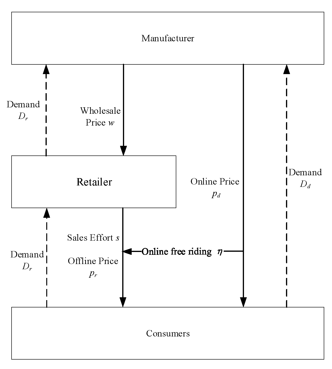
Consider a free-riding dual-channel supply chain composed of a manufacturer and a retailer, where the retailer faces the problem of capital shortage, while the manufacturer has sufficient working capital and can provide funds for the retailer. The capital-constrained retailer makes sales efforts and sells the products at the retail price
. So,
[
11], where
w is the wholesale price of the manufacturer,
φ is the retailer’s marginal profit. Furthermore, the manufacturer also sells products to consumers at prices
through online channels. The capital-constrained retailer can ease its financial pressure through bank loans and deferred payments. At the same time, two kinds of channel power structures are studied; one is the Manufacturer-Stackelberg (M power structure), and the other is the Retailer-Stackelberg (R power structure). Under different scenarios, we give the optimal sales effort and pricing decisions and analyze the financing equilibrium of the enterprise. The structure of the dual-channel supply chain coefficients under free-rider behavior is shown in
Figure 1.
3.2. Mode Setup
In practice, many consumers show free-rider behavior. According to the free-riding dual-channel supply chain literature [
18,
19,
32], the dual-channel supply chain demand function is established:
where
represents the online direct channel demand;
represents the offline traditional channel demand;
a (
) indicates channel market potential;
λ indicates the cross-price sensitivity for the two channels;
indicates the consumer’s free-riding degree; and
s indicates the retailer’s sales effort level. The definitions of all notations are summarized in
Table 2.
In this paper, we use the superscripts and to represent deferred payment and bank loans, respectively. The subscripts and represent the retailer and the manufacturer, respectively. The superscript and indicates the R and the M power structure.
3.3. Basic Assumptions
This study has the following assumptions.
The retailer and the manufacturer are completely rational and risk-neutral [
9,
27].
The sales effort cost is the quadratic function
, and
is the cost coefficient of sales effort [
18,
19].
The initial capital of the retailer is
y and the loan size should be
[
11].
Without losing generality, assuming that the market is completely competitive, the market risk-free interest rate is 0 [
8,
30].
4. Model Solving and Analysis
In this section, the models of the capital-constrained retailer choosing deferred payment and bank credit financing are established, respectively, under the R power structure and M power structure. The equilibrium decisions are compared and analyzed, and the optimal financing strategies of the retailer and manufacturer are obtained.
4.1. Financing Mode in the R Power Structure
This section considers that, under the R channel power structure, the capital-constrained retailer chooses deferred payment or bank loan mode to relieve financial pressure, and discusses the optimal operation strategies and financing modes selection of the retailer and manufacturer.
4.1.1. Deferred Payment
The specific sequence of events in this scenario is as follows: (1) The capital-constrained retailer sets the margin profit and sales effort level ; (2) the manufacturer decides the immediately wholesale , the deferred payment , and online direct price ; (3) the retailer pays the remaining amount to the manufacturer after the end of the sales season.
Therefore, in the deferred payment mode, based on [
8,
18,
36], the manufacturer’s profit and retailer’s profits are presented as follows.
Lemma 1. - (1)
Under the R power structure and deferred payment financing mode, given the interest rate rT, the optimal solutions are as follows: - (2)
The optimal online direct channel demandand the offline distribution channel demandare as follows: - (3)
The optimal manufacturer’s profitand the retailer’s profitare as follows:
According to Lemma 1, the following corollary can be obtained.
Corollary 1. - (1)
,,; If, then;If, then when, ; when, then.
- (2)
; If, then; If, then.
Here,,
.
Corollary 1 (1) shows that the sales effort, the wholesale price and the retail price all decrease with increasing consumer’s free-riding degree η. This is because, with the consumer’s free-riding degree increasing, many more new consumers purchase goods online. Thus, the retailer has to balance investment costs and profit by decreasing sales effort and retail price. The retailer’s decision-making forces the manufacturer to decrease the wholesale price. The online direct price is not monotonically increasing in the consumer’s free-riding degree. It can be found that the impact of free-riding behavior on online prices depends on the cross-price sensitivity λ. If λ is high, the online price is negatively correlated with free-riding behavior; if λ is low, online prices increase first and then decrease with free-riding. This may be because, when the cross-price sensitivity is high, the demand for this channel is greatly affected by the prices of other channels. Note that the offline price decreases with free-riding behavior. Therefore, manufacturers have to reduce the online price to ensure the demand for direct sales channels. When the cross-price sensitivity is low, the demand of this channel is less affected by the prices of other channels, so the manufacturer will increase the online price to improve the marginal profit when the degree of free-riding is low; when free-riding is high, offline retail prices and sales efforts are further reduced, and the manufacturer has to reduce prices to ensure online demand. Therefore, free-riding does not necessarily lead to channel price competition.
Corollary 1 (2) indicates the optimal offline channel demand and free-riding degree of consumers
η negative correlation, but the online channel demand is not monotonically increased in the
η. That is, the online sales channels demand will decrease when the free-riding degree of consumers increases to a certain extent. The reason for this phenomenon is that consumers’ free-riding behavior decreases retailers’ effort input, which finally decreases the demand for offline distribution channels. When
η is relatively high, the retailer further reduces sales efforts and price, thereby reducing the online channel demand. Therefore, free-riding may not increase the online channel demand. Research in the literature [
19] has put forward the same view.
Corollary 2. - (1)
,,,.
- (2)
,.
Corollary 2 (1) shows the relationship between firms’ operational decisions and interest rates
. The high
increases the retailer’s financing cost, thereby hindering the investment of retailers’ sales efforts. Thus, high-interest rates will reduce retailers’ sales efforts. Note that, the offline price and online price increase with the increase in
. However, the wholesale price decrease with the increased interest rate
. As a result of the increase in
, the retailer has to balance the financing, investment, and purchase cost by increasing offline retail prices. As the manufacturer can obtain the retailer’s loan cost, this increases the online price and the loan cost of the retailer. This means that deferred payment can avoid channel price competition in the dual-channel supply chain. This further verifies the views of Qin et al. [
34].
Corollary 2 (2) shows that the demand for the distribution channel and online direct channel always decreases with the increased interest rate . On the one hand, the retailer will reduce sales effort investment to alleviate the financing pressure, which decreases the demand for distribution channels. On the other hand, the manufacturer guides consumers to shop in the distribution channel through a price strategy in order to increase the financing cost of the retailer, thereby hurting demand for the direct channel.
4.1.2. Bank Loans
The specific sequence of events in this scenario is as follows: (1) The capital-constrained retailer sets the retail margin , and sales effort level , and applies for the loan from the bank; (2) The manufacturer decides the sales price and the wholesale price ; (3) The retailer obtains the loan from the bank and then purchases products from the manufacturer; (4) the retailers repay loans and interest at the end of the sales period.
Therefore, in the bank loans mode, based on [
8,
18,
36], the profit function of manufacturers and retailers under bank loans is presented as follows.
Lemma 2 - (1)
The optimal solutions are as follows: - (2)
The optimal online channel demandand the offline channel demandare as follows: - (3)
The manufacturer’s profit and the retailer’s profitare as follows:Here,,.
According to Lemma 2, the following corollary can be obtained.
Corollary 3. - (1)
,,; If λis high, then ;If λis low, then when,;when,.
- (2)
; If ,then ; If ,then .
Here, ,
.
Corollary 3 (1) indicates the sales effort, the retail and the wholesale price reductions, with the consumer’s free-riding degree η. The influence of free-riding behavior on online sales prices depends on cross-price sensitivity. This conclusion is similar to Corollary 1 (1). Therefore, the principle will not be elaborated on in detail.
Corollary 3 (2) shows that the optimal offline channel demand decreases with the increase of η, but the optimal online channel demand is not monotonically increased in the η. This conclusion is similar to Corollary 1 (2). Therefore, the principle will not be elaborated on in detail.
The above phenomenon shows that, under the R power structure, the impact of consumer free-riding behavior on participants’ operational decisions and market demand has nothing to do with the financing model.
Corollary 4. - (1)
,,,.
- (2)
,.
Corollary 4 (1) indicates that the sales effort, the online sales price, and the wholesale price all reduce with the increase in . The reason is that, with the increase in , the retailer has to balance profit and total cost by decreasing the sales effort and increasing offline retail prices. As the retailer’s loan cost flows out of the chain, the manufacturer has to avoid decreasing market total demand by decreasing online sales price and wholesale price. This conclusion is different from the conclusion in Corollary 2 that online sales price is negatively correlated with interest rate . That is, the impact of the interest rate on the online price is related to the financing model.
Corollary 4 (2) indicates that the optimal offline channel demand reduces with the increase of , but the optimal online channel demand increases with the . The reason for this phenomenon is that the retailer’s financing costs flow outside the supply chain. The increase in will inevitably decrease the sales effort, and then reduce the demand for the distribution channel. The manufacturer has to ensure its profit by increasing the demand quantity of direct channels.
4.1.3. Deferred Payment vs. Bank Loans
In this section, we aim to examine the optimal financing model of the two companies under the R power structure.
Theorem 1. If,then
- (1)
,,,.
- (2)
,.
Theorem 1 (1) indicates that, if
, then the sales effort and online direct price of bank loans are lower than that of deferred payment. However, the manufacturer’s price strategies in deferred payment are lower than that of bank loans. The reason for this phenomenon is that the manufacturer has three roles: the product provider, the seller, and the financing provider in the deferred payment mode. Thus, the manufacturer could balance financing revenue, the profit of wholesale products, and the profit of direct sales products by decreasing wholesale prices and increasing online direct sales prices. The high online direct sales price discourages consumers from purchasing products from the online channel, which encourages the retailer to be willing to make higher sales efforts. The retailer can obtain more market demand by providing lower retail prices, which can make up for the financing cost to a certain extent (
Appendix D).
Theorem 1 (2) indicates that, if , then the optimal offline channel demand in bank loans is lower than that of deferred payment. This is because the sales effort in bank loans is lower than that deferred payment, and the distribution retail price is lower. In addition, in bank loan mode, the optimal online channel demand is positively correlated with the interest rate. However, the optimal online channel demand under the deferred payment is badly impacted by the interest rate. Thus, the online demand under the bank loan mode is higher.
Theorem 2. If,then
- (1)
For the retailer:.
- (2)
For the manufacturer: when, ; when,.
Here,.
Theorem 2 (1) shows that, if
, then the retailer always obtains a lower profit under bank loans than that deferred payment. Although the retailer sacrifices part of its retail price under deferred payment, due to higher sales efforts and lower wholesale prices, the market demand for offline channels under bank loans is lower than that of deferred payment. Thus, deferred payment is the best financing model for the retailer. Theorem 2 (2) reveals the willingness of the manufacturer to solve capital problems for the retailer. When initial capital is low, it would choose to provide deferred payment. Otherwise, bank loans are better for the manufacturer. Therefore, there is a critical value in the initial capital of the retailer. To the left of the critical value, deferred payment is the financing equilibrium of the manufacturer and the retailer. To the right of the threshold, the retailer and the manufacturer have conflicting financing decisions (
Appendix E).
4.2. Financing Mode in the M Power Structure
This section considers that, under the M power structure, the retailer chooses deferred payment or bank loan mode to relieve the capital-constrained problem, and discusses the optimal operation strategies and financing modes selection of the retailer and manufacturer.
4.2.1. Deferred Payment
The specific sequence of events in this scenario is as follows: (1) The manufacturer decides the immediately wholesale , the postponed payment , and online direct price ; (2) The capital-constrained retailer sets the retail price and sales effort level ; (3) The retailer pays the remaining amount to the manufacturer after the end of the sales season.
Similar to
Section 4.1.1, in the deferred payment mode under the M power structure, the profits of manufacturers and retailers are presented as follows.
Lemma 3. - (1)
The optimal solutions are as follows:Here,.
- (2)
The optimal online channel demandand the offline channel demandare as follows: - (3)
The manufacturer’s profit and the retailer’s profit are as follows:
According to Lemma 3, the following corollary can be obtained.
Corollary 5. - (1)
.
- (2)
.
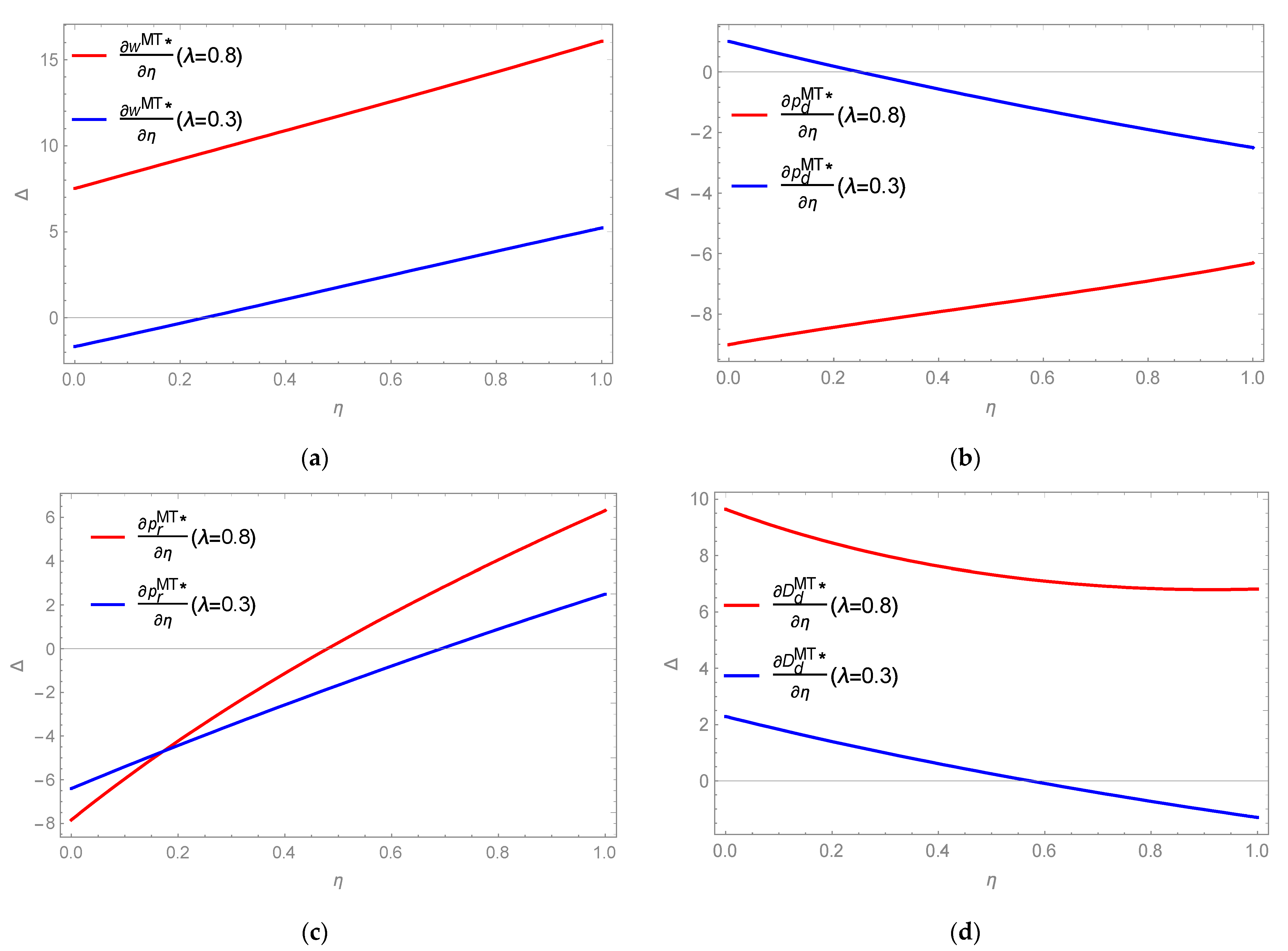
Corollary 5 (1) shows the influence of consumers’ free-riding degree on the sales effort. When consumers have a higher free-riding degree, the retailer would reduce the cost of the loans by decreasing the sales effort investment. Corollary 5 (2) shows that the optimal offline channel demand reduces with the increase in consumers’ free-riding degree. This conclusion is similar to Corollary 1 (2), thus the principle will not be elaborated on in detail. As the derivatives of the wholesale price, online sales price, offline sales price, and online market demand regarding consumer free-riding degree are complex under the M power structure, thus we analyze the influence of free-riding degree on pricing strategy and online channel demand through numerical simulation (
Appendix B).
Based on [
9,
11,
18,
19], we here assume that potential market demand, sales efforts cost coefficient, and financing interest rate are
, and
, respectively. The cross-price sensitivity
λ is taken values of
and
, respectively.
Figure 2a–d shows the influence of free-riding on the wholesale price, online sales price, offline retail price, and online channel market, respectively.
Figure 2a shows that, when the cross-price sensitivity
λ is high
, the wholesale price increases with the degree of free riding; when the cross-price sensitivity
λ is low
, the wholesale price decreases first and then increases with free riding. This conclusion is different from (1) in Corollary 1 and Corollary 3 and is also different from the conclusion in the literature [
18,
19].
Figure 2b shows that, when the cross-price sensitivity
λ is high
, the online sales price reduces with the degree of free riding; when the cross-price sensitivity
λ is low
, the online sales price decreases first and then increases with free riding. This may be because, under the M power structure and deferred payment mode, the manufacturer has pricing priority and can obtain the financing cost of the retailer. When
λ is high, the manufacturer increases the wholesale price and reduces the online price. On the one hand, this can increase the financing pressure of the retailer (the financing revenue increases), and on the other hand, it can increase the online channel demand (see
Figure 2d) (the sales revenue increases). When
λ is low, the manufacturer’s reduction of online prices cannot effectively increase online channel demand. Therefore, when consumers have a low degree of free-riding, the manufacturer will reduce the wholesale price to encourage the retailer to increase the order number, and increase the online price to increase the sales margin profit. When consumers have a higher degree of free-riding, the retailer’s orders will decrease, and the manufacturer will increase the wholesale price, increase the profit margin of offline sales, and reduce the online price to attract more consumers. Thus, when the cross-price sensitivity
λ is high
, online channel demand increases with the degree of free riding. When cross-price sensitivity
λ is low
, online channel demand increases first and then decreases with the degree of free riding.
Figure 2c shows that the offline retail price reduces first and then increases with the degree of free-riding, which has nothing to do with the cross-price sensitivity. This means that in the manufacturer-led dual-channel supply chain, free riding does not always reduce the price of the retailer. When the free-riding degree increases to a certain extent, the retailer will increase the retail price instead.
Corollary 6. - (1)
,,. If, then; If, then .
- (2)
,.
Here,.
Corollary 6 (1) shows the impacts of the interest rate of deferred payment on the sales effort and the firms’ price strategies. When the manufacturer provides a high-interest rate deferred payment for the retailer, the retailer has to balance operation total cost by reducing sales effort at first. Furthermore, the retailer also reduces retail prices to avoid a decrease in the demand quantity of offline channels when is low. The retailer has to raise retail prices to further alleviate the financing pressure when the interest rate increases to a certain extent. Furthermore, the online sales price and wholesale price always decrease with the increase in interest rate. This is because, on the one hand, the loss of profit on the decrease of the wholesale price can be made up for by the financing revenue. On the other hand, the online sales price decrease can raise the demand quantity for offline direct channels.
Corollary 6 (2) indicates the impacts of , the optimal offline and online channel demand. When the manufacturer provides a high-interest rate deferred payment service for the retailer, it is bound to guide consumers to shop in distribution channels through price strategies, in order to increase the retailer’s financing cost, which decreases the online channel demand. However, the retailer will decrease the sales level to alleviate the financial pressure, thereby hurting the demand for distribution channels.
4.2.2. Bank Loans
The specific sequence of events in this scenario is as follows: (1) The manufacturer decides the sales price and the wholesale price ; (2) The capital-constrained retailer sets the retail price , and sales effort level , and applies for the loan from the bank; (3) The retailer obtains the loan from the bank and then purchase products from the manufacturer; (4) the retailers repay loans and interest at the end of the sales period.
Similar to
Section 4.1.2, in the bank loan mode under the M power structure, the profits of manufacturers and retailers are presented as follows.
Lemma 4. - (1)
The optimal solutions are as follows:Here,.
- (2)
The optimal online channel demandand the offline channel demandare as follows: - (3)
The manufacturer’s profitand the retailer’s profitare as follows:
According to Lemma 4, the following corollary can be obtained. Since the influence of free-riding behavior under the bank loan mode on the optimal decision-making and market demand of supply chain participants is similar to the conclusion under the deferred payment mode, this section will not discuss it in detail.
Corollary 7. - (1)
,,,.
- (2)
,.
Corollary 7 (1) indicates the influences of the interest rate on the sales effort, and the firms’ price strategies. It can be found that the sales effort, the wholesale, and the online sales price all decrease with the increase in , even though the retailer increases the offline sales price. That is, the retailer balances operational total cost by decreasing sales effort and increasing the retail price. The manufacturer alleviates the reduction of offline channel demand by decreasing the wholesale price, while it reduces the online direct price to attract consumers to spend online, in order to ensure its profit.
Corollary 7 (2) indicates that the offline distribution channel demand decreases with , but the optimal online channel demand increases with . This conclusion is similar to Corollary 4 (2), thus the principle will not be elaborated on in detail.
4.2.3. Deferred Payment vs. Bank Loans
By comparing the deferred payment and bank loans, we discuss which financing model is more conducive to sales efforts under the M power structure.
Theorem 3. If, then
- (1)
,,,.
- (2)
,.
Theorem 3 (1) indicates that, if , then the sales effort and online direct price of bank loans are always lower than that deferred payment. However, the offline retail price and the wholesale price of deferred payment are always lower than bank loans. For the following reasons, the manufacturer can obtain the financing revenue under a deferred payment mode. The loss of the low wholesale price can make up for the financing cost of the retailer. With the low wholesale price, the retailer is willing to increase sales effort and decrease the retail price. The high online sales price can not only obtain high direct sales marginal profits, but also encourage consumers to spend offline, and then obtain higher financing costs for the retailer.
Theorem 3 (2) indicates that, if , the offline channel demand of the deferred payment is higher than that of bank loans. However, the online direct channel demand for deferred payment is lower than bank loans. This conclusion is similar to Theorem 1 (2), thus the principle will not be elaborated on in detail.
Theorem 4. If, then
- (1)
For the retailer:.
- (2)
For the manufacturer: when,;when,.
Here,.
Theorem 4 (1) indicates that if
, then the retailer’s profit is higher under deferred payment. That is, under the M power structure, the deferred payment is the best financing model for the retailer. Theorem 2 (2) reveals the willingness of the manufacturer to provide financing services for the retailer. If the initial capital
y is relatively low, then the manufacturer would choose to provide deferred payment. Otherwise, the manufacturer earns more on bank loans than on deferred payments. Therefore, there exists a Pareto zone
, where deferred payment is beneficial to both the manufacturer and the retailer. In other words, when the initial capital meets certain conditions, deferred payment is the financing equilibrium for the manufacturer and retailer (
Appendix F).
5. Comparison between the R and M Power Structure
This section explores the influences of power structure on pricing strategies and sales effort levels by comparing the R and the M power structure under each financing mode.
5.1. Under the Deferred Payment
We first analyze the optimal decision-making of the supply chain in the R and M power structure under the bank loan mode.
Theorem 5. ,,,.
Theorem 5 indicates that the wholesale price and the sales effort under the R power structure are lower than that under the M power structure. However, the online sales price and the offline price under the M power structure are lower than that under the R power structure. The reason for this phenomenon is that the retailer could give priority to pricing under the R power structure. Therefore, although the retailer offers higher retail prices, it is reluctant to increase sales efforts level under the R model. Furthermore, the retailer’s operation decision forced the manufacturer to reduce the wholesale price. However, the retailer has to raise sales effort levels and reduce retail prices to ensure its profit under the M power structure. This means that the M power structure is more conducive for the retailer to make sales efforts, reduce online and offline sales prices, and increase market total demand (
Appendix G).
5.2. Bank Loans
We then compared the operational decision-making in the two power structures under bank loans.
Theorem 6. ,,,.
Theorem 6 shows that under bank loans, the sales effort and the wholesale price under the R power structure are lower than that under the M power structure. However, the online sales price and the offline price under the M power structure are lower than that under the R power structure. This conclusion is similar to Theorem 3. It shows that, no matter what kind of financing mode, the M power structure has more advantages than the R power structure in retailer sales effort level under the consumers’ free-riding. However, the R power structure has more advantages than the M power structure in online and offline sales prices.
6. Numerical Analysis
In this section, based on verifying the above conclusions through numerical simulation, we discuss the impact of cross-price sensitivity on the profits of the retailer and manufacturer and further explore which power structure is more beneficial to the retailer and manufacturer under different financing modes. Based on [
9,
11,
18,
19], we here assume that potential market demand, sales efforts cost coefficient, financing interest rate, and initial capital are
,
and
,
respectively. The cross-price sensitivity
λ is taken values of
and
respectively. We analyze the influence of free-riding degree and financing interest rate on the optimal operation strategy and profit of both parties in the supply chain under the R/M power structure. The results are shown in
Table 3 and
Table 4.
From
Table 2 and
Table 3, we can find the following: (1) Compared with the bank loan mode, the retailer can always obtain higher profits under the deferred payment mode. However, when the cross-price sensitivity
λ is relatively low
, the bank loan is the optimal financing strategy for the manufacturer under the R power structure; otherwise, deferred payment is the optimal financing strategy for the manufacturer under the M power structure. In addition, the manufacturer is always willing to provide financing services for the retailer when
λ is relatively high
. This means that the power structure will not affect the financing strategy choice of capital-constrained retailers, but will affect the financing decisions of manufacturers.
(2) Under the R power structure, if the retailer chooses to defer payment, its profit is under cross-price sensitivity and is the same; if the retailer chooses a bank loan, its profit is higher when under cross-price sensitivity λ is relatively low . Under the M power structure, the retailer’s profit is higher when λ is relatively high under the deferred payment/bank loans. The above phenomenon shows that in the manufacturer-led dual-channel supply chain, high cross-price sensitivity is conducive to financial constraints on retailers; in the retailer-led dual-channel supply chain, if retailers choose deferred payment, their profit is not affected by cross-price sensitivity. If it chooses bank credit, then low cross-price sensitivity is more beneficial to capital-constrained retailers.
(3) For the manufacturer: under deferred payment/bank loans, its profits under the M power structure are higher than those under the R power structure. For the retailer: under deferred payment, its profits under the R power structure are higher than those under the M power structure; However, under bank loans, its profits under the R power structure are high when cross-price sensitivity λ is relatively low ; its profits under M power structure are high when λ is relatively high . This means that in the dual-channel supply chain with a capital-constrained retailer, manufacturers should give priority to publishing price strategies, and retailers should decide whether to give priority to publishing operation strategies according to financing mode and cross-price sensitivity.
(4) Under the R/M power structure and deferred payment/bank loans, free-riding behavior always reduces retailers’ sales efforts and damages the profits of retailers and manufacturers. The financing interest rate does not necessarily reduce the profits of retailers, which depend on their initial capital, but it will certainly damage the profits of manufacturers. Therefore, manufacturers should provide retailers with zero interest rate deferred payment services.
7. Discussion
To validate the robustness of the model, we extend our model by considering that sales effort level is an exogenous variable and that consumers have channel preferences. The sequence of events is the same as already mentioned, except that the retailer does not determine the level of sales effort.
In consumer channel preference, based on [
5,
35] research, the market demand can be denoted as
where
θ indicates the proportion of consumers’ preference for offline channels, and
indicates the proportion of consumers’ preference for online channels.
In this section, we study the impact of sales effort level and channel preference on firms’ financing mode choice. The result is shown in Theorem 7.
Theorem 7. If ,then
- (1)
In the R mode,,.
- (2)
In the M mode,,.
where,,
.
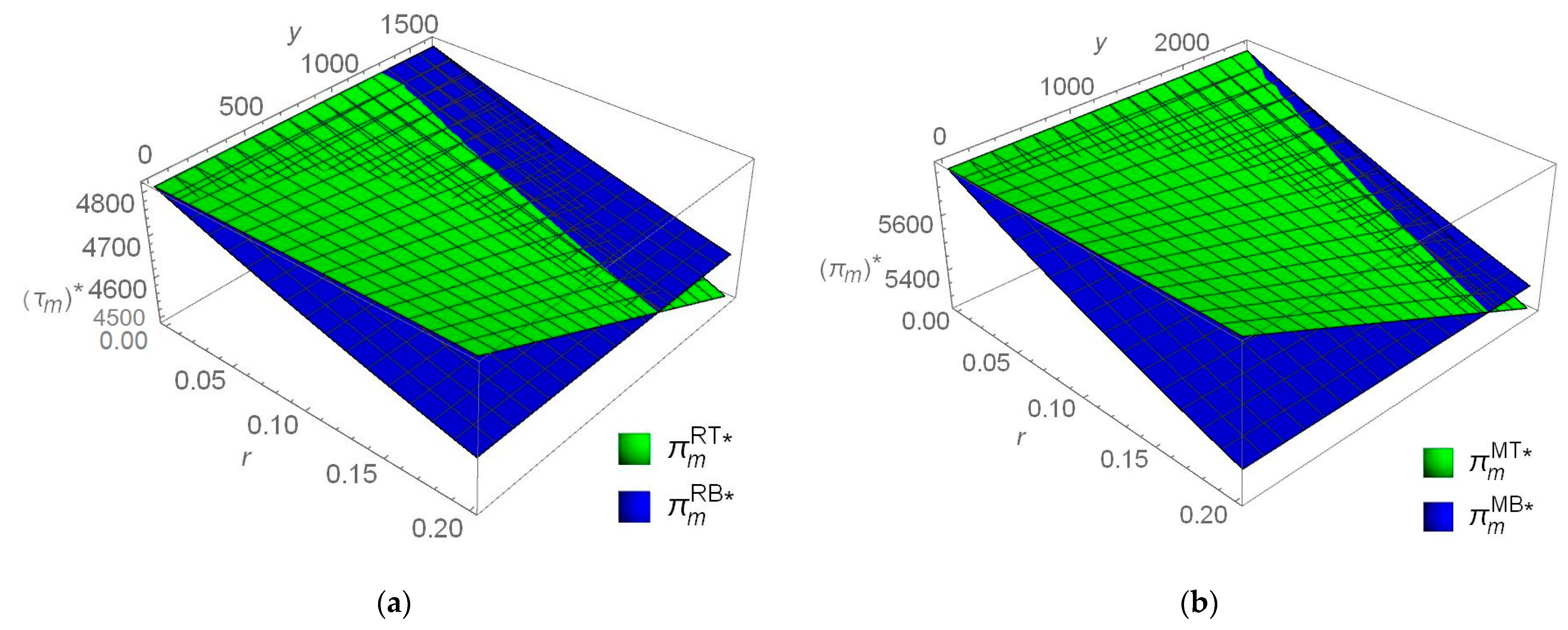
Theorem 7 (1) shows that the retailer achieves higher profit under the deferred payment mode and that the manufacturer’s choice of financing mode relies on the initial capital, under sales efforts level as an exogenous variable and consumers’ channel preference. The retailer and manufacturer make more profits under deferred payment when the initial capital is fairly low . That is, deferred payment acts as the financing balance under the R power structure. Theorem 9 (2) shows that, under the M power structure, the retailer favors the deferred payment mode, and the manufacturer earns more under bank loans when the initial capital is high . Conclusively, under the R and M power structures, the sales efforts as exogenous variables and the consumers’ channel preference do not influence the choice of the financial model.
Figure 3 reveals the relationship of the manufacturer’s profit between the R and the M modes when the consumers have channel preference, and sales efforts level is an exogenous variable. Based on [
9],
,
,
,
,
,
can be seen. Therefore, under the R power structure, the retailer’s original funds
can be seen; under the M power structure, the retailer’s initial capital
can be seen. It can be found that, although the consumers prefer offline channels to online channels and sales efforts act as an exogenous variable, the power structure always affects the initial capital threshold, and then influences the manufacturer’s financing policy choice. Therefore, the correlation between R and M power structures has nothing to do with the fact that sales efforts are exogenous variables or with consumer channel preferences.
Next, the link between the firms’ profit and the “free-riding” degree is shown in Theorem 8.
Theorem 8. - (1)
, ,,.
- (2)
,,,.
Theorem 8 (1) reveals that the manufacturer’s profits increase with the addition of the “free-riding” degree when sales efforts are an exogenous variable, which does not have anything to do with the power structure and financing model. This implies that the manufacturer benefits from consumers’ free-riding behavior when the retailer does not make decisions on the sales effort level. This may be because the sales effort level as the exogenous variable is not negatively affected by the free-riding performance of consumers, and the manufacturer can also avoid the negative influence of consumers’ free-riding performance through price strategy, in order to improve its profits. Theorem 8 (2) shows that the consumers’ free-riding performance always reduces the profit of the retailer; this finding is consistent with the situation that sales effort level is an endogenous variable. In other words, whether the retailer decides on the level of sales effort or not, the free-riding performance of consumers will always reduce the retailer’s profits (
Appendix G).
In summary, consumers’ channel preference changes the optimal pricing decisions, and sales effort as an exogenous variable will change the influence of consumers’ free-rider behavior on manufacturers’ profits, but does not affect the choice of financing mode, which indicates that the fundamental model’s results are robust.
8. Conclusions
Considering the free-riding effect and power structure, this study examines a dual-channel supply chain consisting of a retailer and manufacturer, where the retailer faces the problem of constrained capital and the manufacturer has sufficient funds to offer financing services to the retailer. Furthermore, the retailer can also relieve financial pressure through bank loans. We get some valuable conclusions by comparing and analyzing the profits and operation strategies of firms.
- (1)
Financing Decision-making
The optimal financing strategies of retailers and manufacturers, by comparing the deferred payment and bank loan modes under the R and M power structures, are obtained. The results show that, under each power structure, deferred payment is always the optimal financing strategy for the retailer. The initial capital has a range that allows the manufacturer to benefit from deferred payment modes; otherwise, bank loans are the manufacturer’s optimal financing decision. The choice of financing strategy has nothing to do with free-riding behavior. Furthermore, the retailer purchases more products under deferred payment and works harder to sell them than under bank loans. High-interest rates do not necessarily decrease the retailer’s profit, but will certainly decrease the manufacturer’s profit.
- (2)
Influence of power structure
It is found that the financing decisions of the capital-constrained retailer are independent of the power structure, and it always benefits from intra-supply chain financing (deferred payment). However, for the manufacturer, power structure affects the initial capital threshold, and then influences the financing strategy choice of the manufacturer. Compared with the R power structure, sales effort level and offline channel demand are higher under the M power structure. Furthermore, manufacturers should give priority to publishing price strategies, while retailers should decide whether to give priority to publishing price and sales effort strategies according to the financing mode and cross-price sensitivity.
- (3)
Price and sales effort decisions
When the degree of free riding is low, it can increase the online market demand, but it will damage the profits of node enterprises in the supply chain. The influence of free-riding on price depends on the power structure and cross-price sensitivity, while the influence of interest rate on price depends on the power structure and financing model. In addition, free-riding may not aggravate the channel price competition between retailers and manufacturers.
This paper has the following implication: this study attempts to enrich the relevant research on supply chain finance and think about a more accurate background for dual-channel supply chain financing. This study considers the reality of the power structure and free riding, and analyzes the optimal operation decision and financing strategy choice of a dual-channel supply chain. In addition to its contributions to the literature, this paper also draws some insights into supply chain management. (1) In the dual-channel supply chain, the traditional retailer does not need to consider the power structure when financing, but the manufacturer should comprehensively consider the power structure and the initial capital of the retailer. In particular, it is more advantageous for the manufacturer to provide financing services at zero interest rates. (2) It may not be beneficial for retailers to give priority to publishing prices, which depends on the financing model and cross-price sensitivity, and manufacturers should always give priority to publishing price strategies. Compared with Retailer-Stackelberg, the Omni channel sales price is lower and the level of sales efforts is higher under Manufacturer-Stackelberg. (3) Delayed payment is conducive to easing channel price competition and strengthening internal cooperation in the supply chain.
This paper explores the financing decisions of a dual-channel supply chain consisting of a retailer and a manufacturer under the one-way free-rider effect. Future research can be expanded considering the following aspects: first, studying the choice of supply chain financing strategy under the two-way free rider effect; second, future research can consider the risk aversion behavior of the manufacturer and retailer; third, future research can consider the situation of uncertain market demand.


