
The Impact of Rainfall on Urban Human Mobility from Taxi GPS Data


Abstract
:1. Introduction
2. Study Area and Data
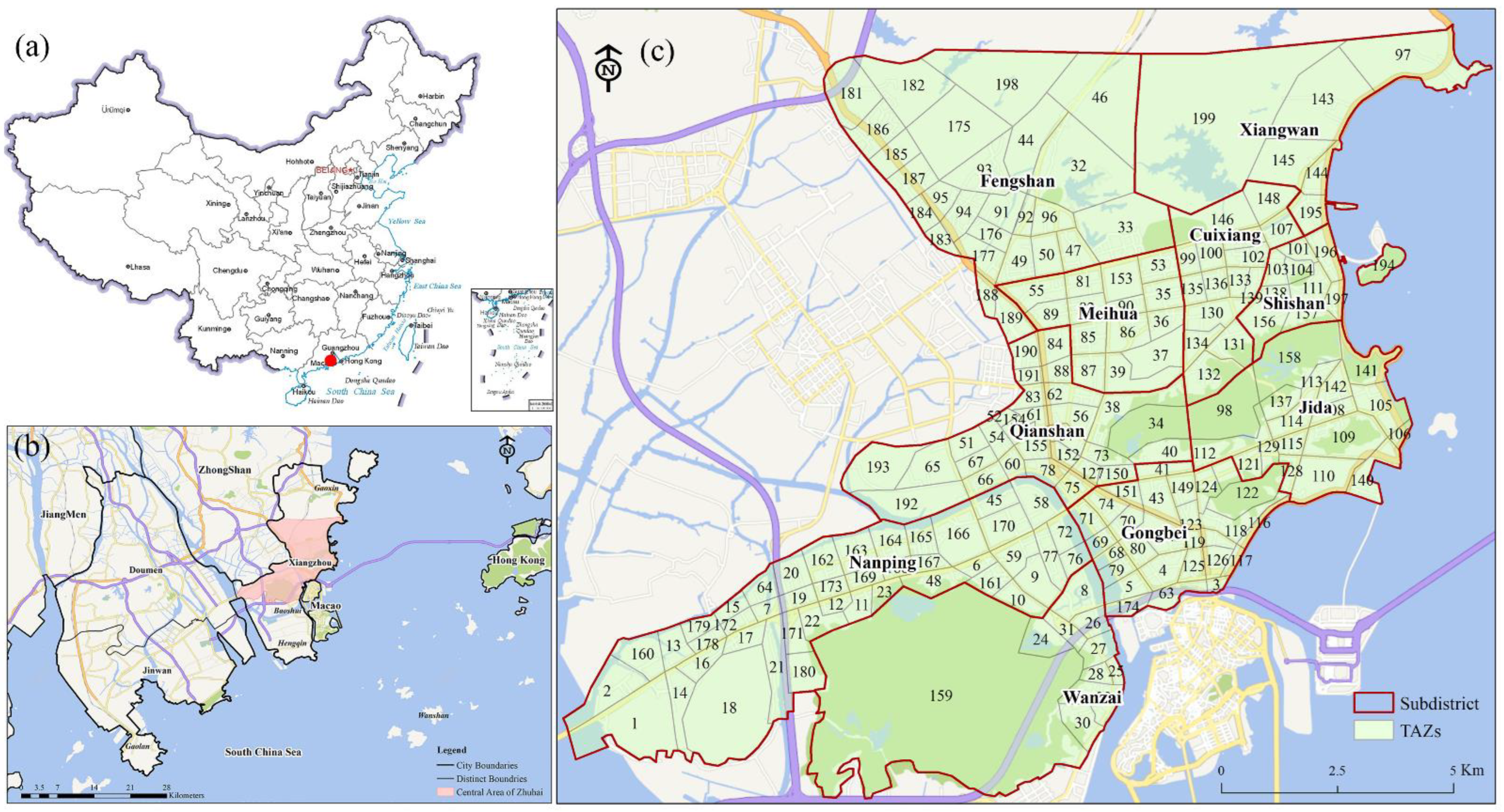
2.1. Case Study: Zhuhai, China
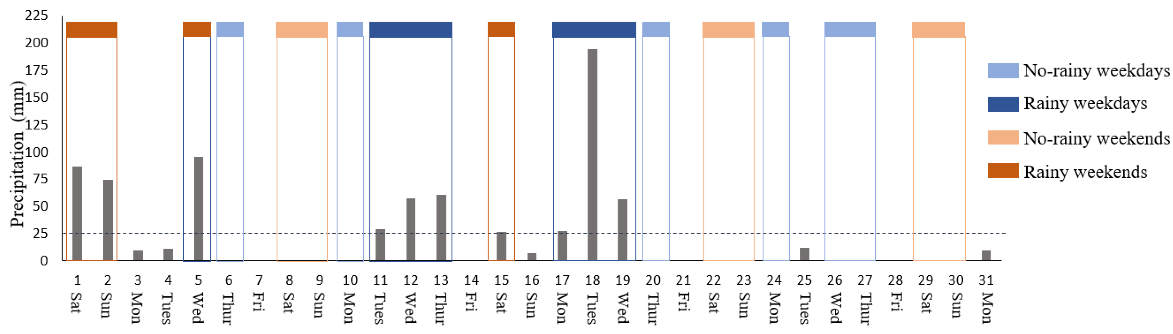
2.2. Data Source
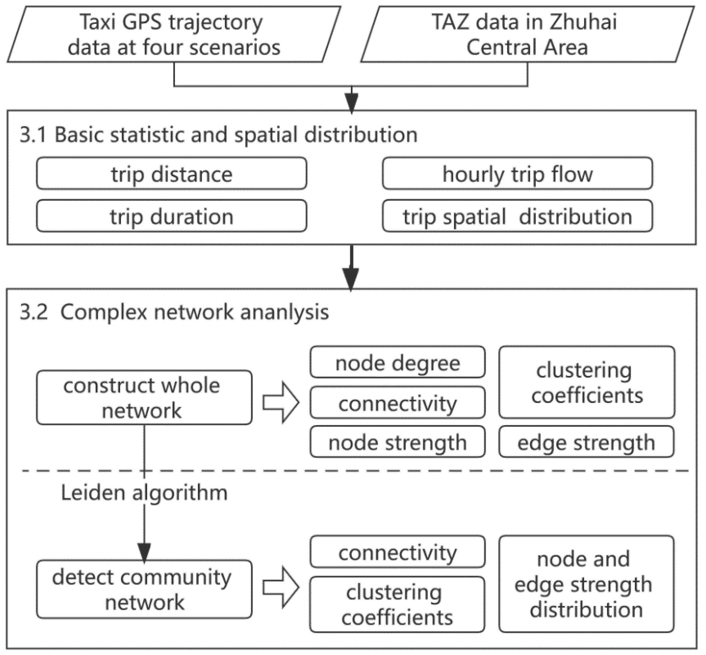
3. Methodology
3.1. Basic Mobility Characteristics
3.2. Complex Network Analysis
3.2.1. Network Construction and Community Detection
3.2.2. Statistical Indicators of Network
4. Results
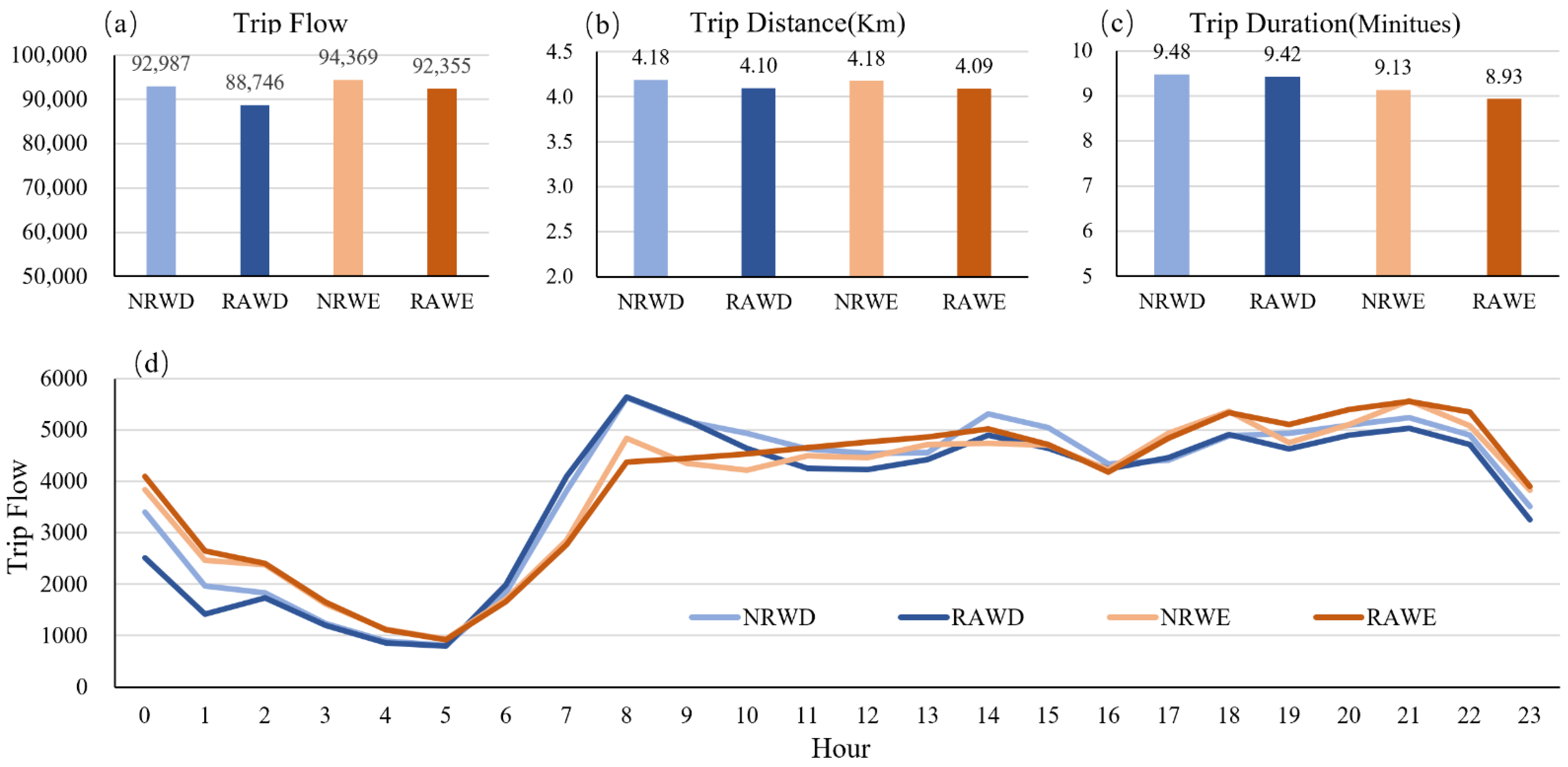
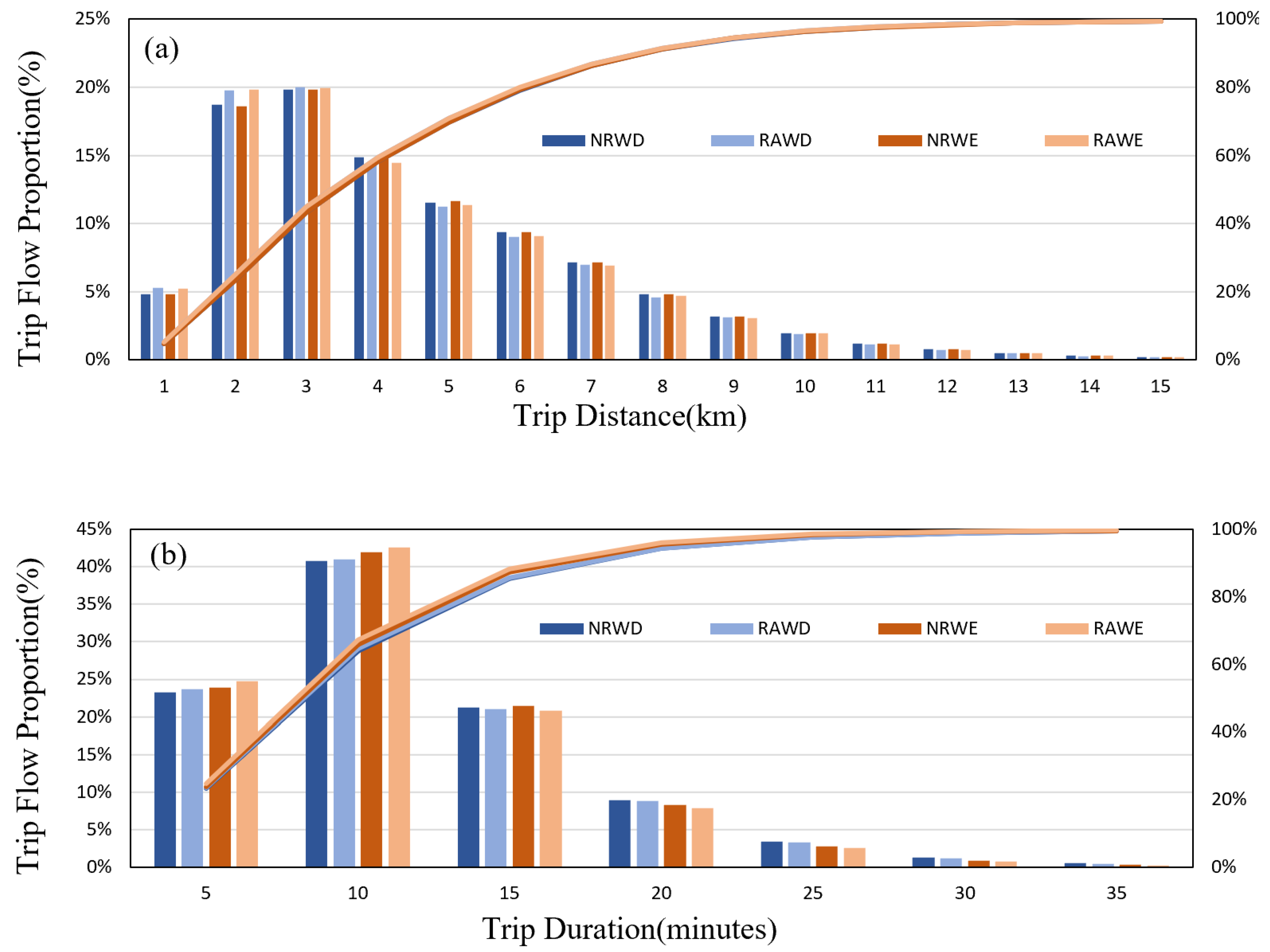
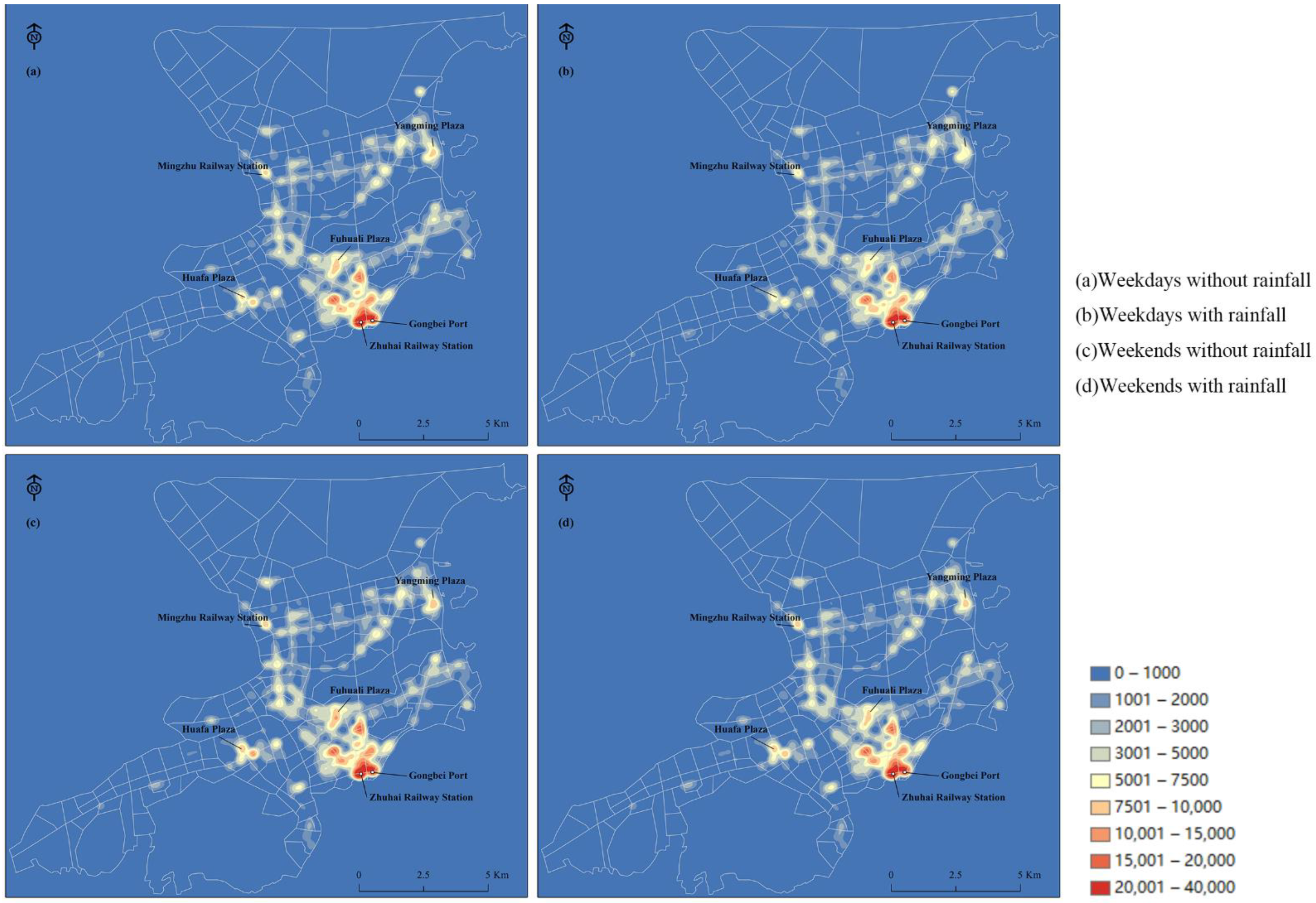
4.1. Basic Statistics and Spatial Distribution of Trip Data
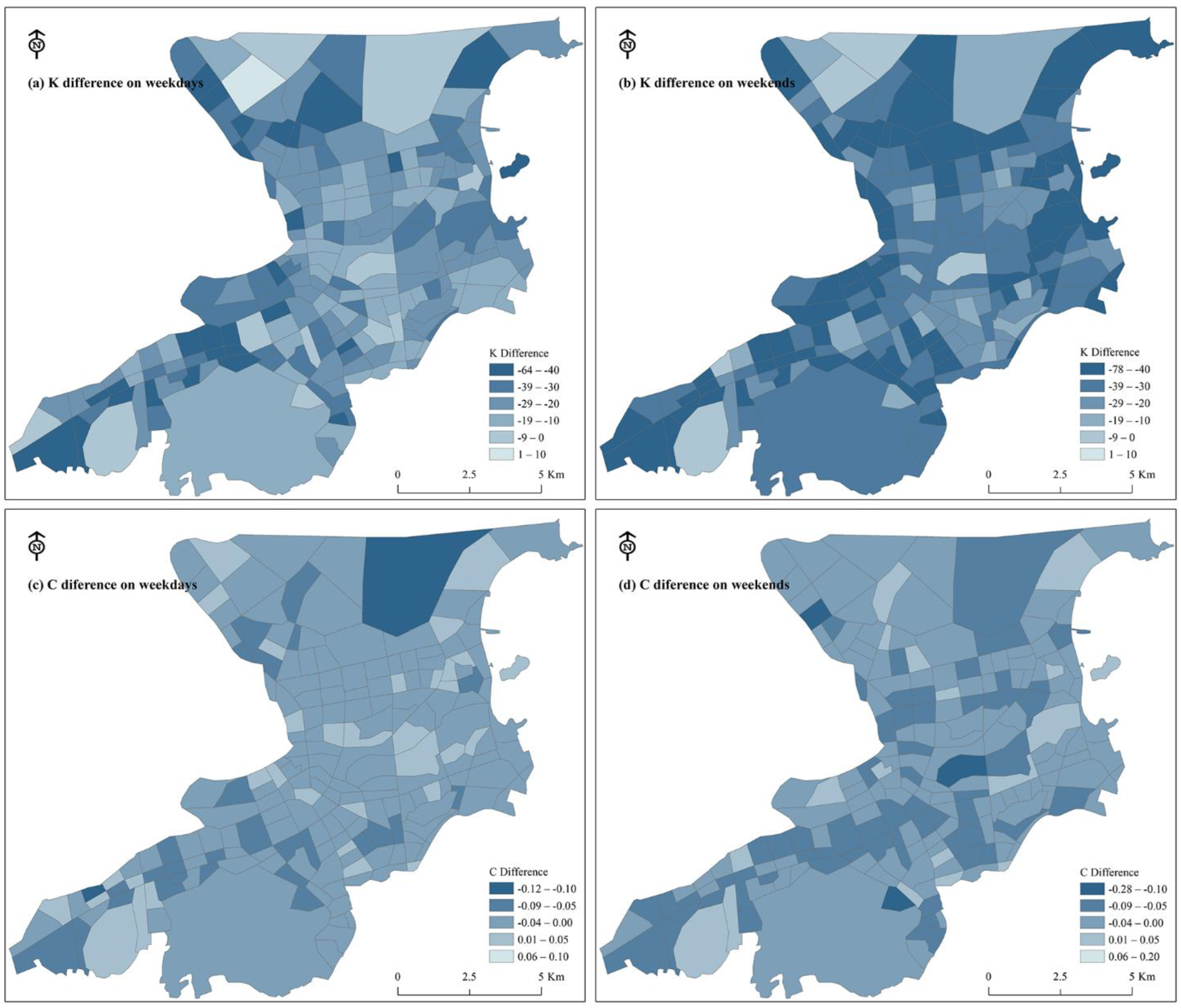
4.2. Complex Network-Based Analytical Indicators
4.2.1. Indicator Analysis of Whole Network
4.2.2. Indicators Analysis of Community Network
5. Summary and Discussion
6. Conclusions
- (1)
- Taxi GPS data are highly informative and exploitable in the field of human mobility analysis. Using the location and times at which passengers were picked up and dropped off in taxi trip GPS data, we can analyze activity levels across the city and the way people move around the city;
- (2)
- Rainfall has a reducing effect on trip flow whether on weekdays or at weekends, as well as on trip distance and trip duration, but has no significant impact on the appearance and duration of peak hours. From the spatial distribution of passengers, it is evident that rainfall has little effect on most hotspots, with the exception of a few commercial centers;
- (3)
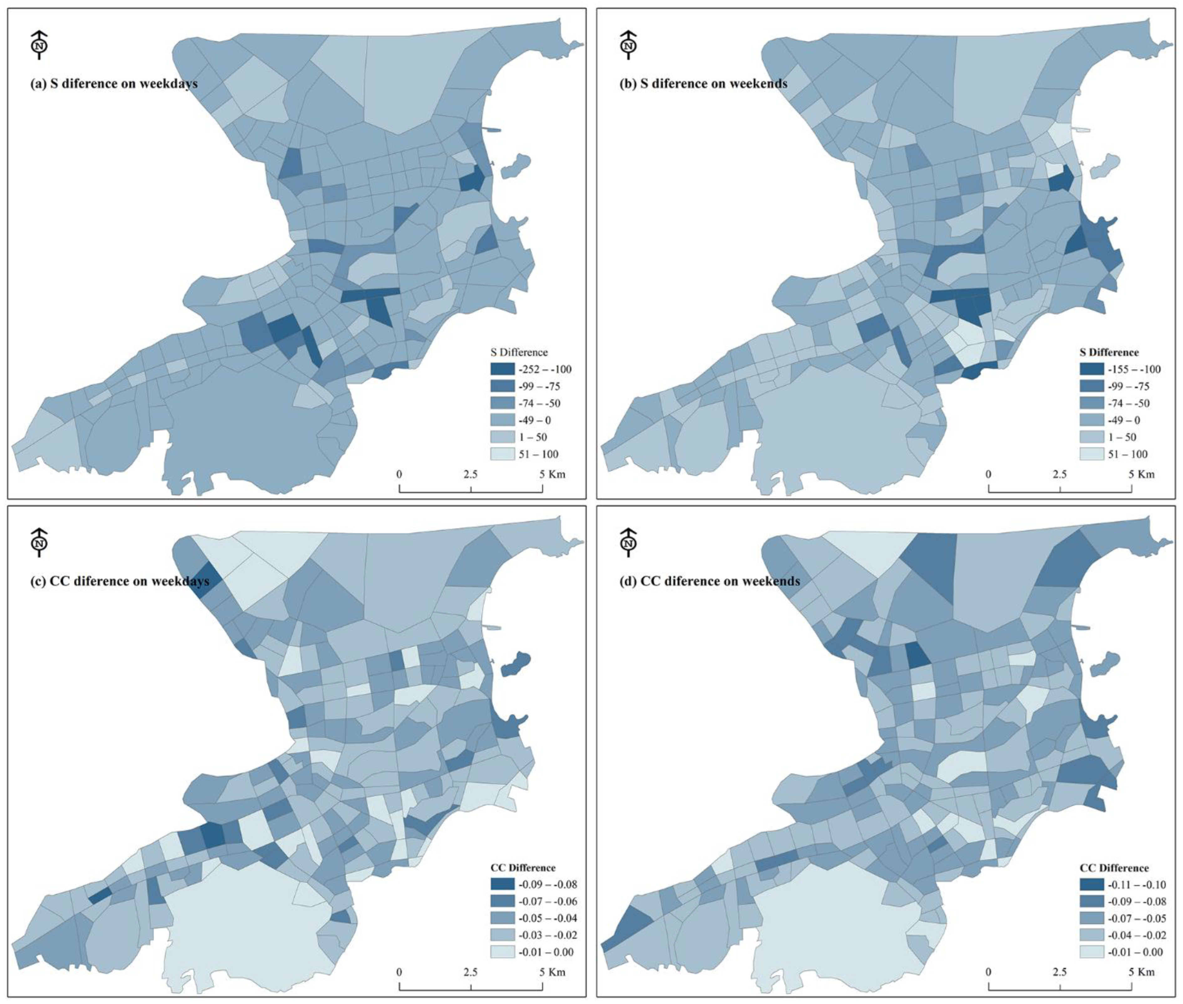
- From the perspective of the whole mobility network, rainfall has a significant effect on the network indicators. For instance, the edges of the network and the average degree of nodes decreased significantly on days with rainfall. Node and edge strength in some commercial areas declined significantly on the days with rainfall;
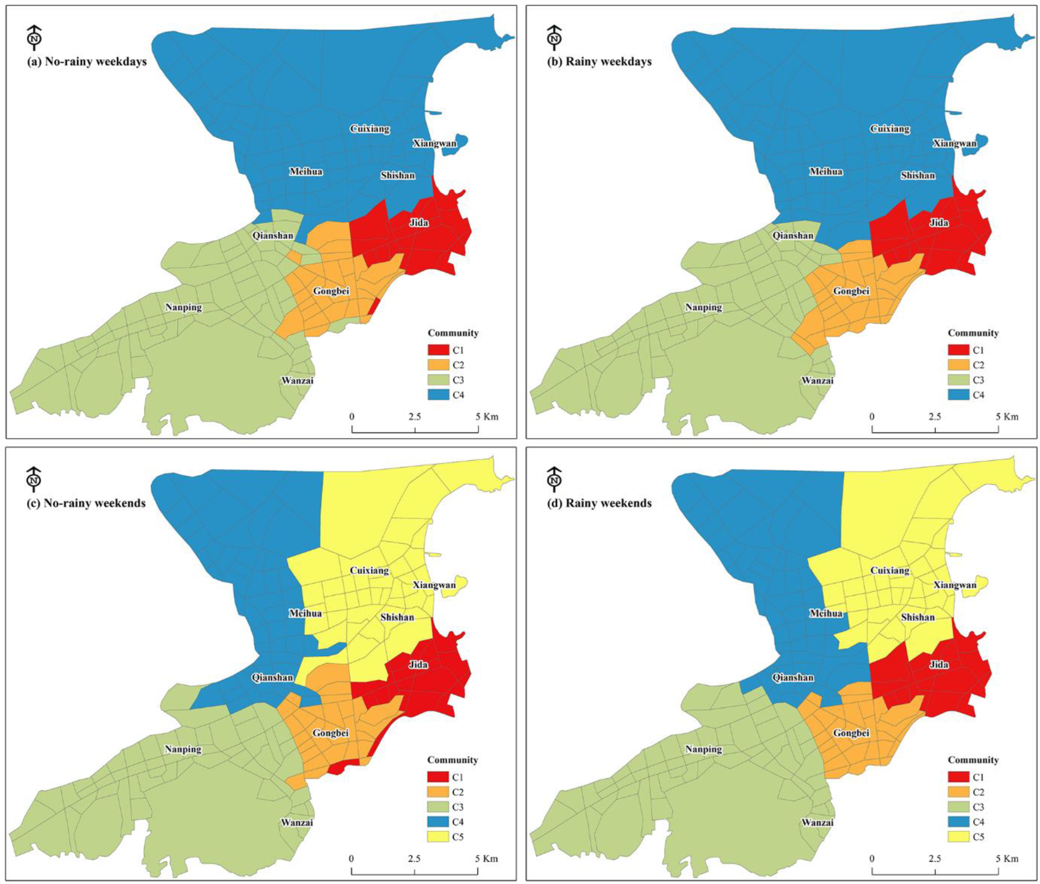
- (4)
- There were more mobility communities were detected on weekends than on weekdays. The number of communities on weekdays and weekends did not change because of rainfall. For communities located in transportation hubs or port areas, the changes in network indicators were opposite to those of other communities.
Author Contributions
Funding
Institutional Review Board Statement
Informed Consent Statement
Data Availability Statement
Acknowledgments
Conflicts of Interest
References
- Xu, M.L.; Fu, X.; Tang, J.Y.; Liu, Z.Y. Effects of weather factors on the spatial and temporal distributions of metro passenger flows: An empirical study based on smart card data. Prog. Geogr. 2020, 39, 45–55. [Google Scholar] [CrossRef]
- Barbosa, H.; Barthelemy, M.; Ghoshal, G.; James, C.R.; Lenormand, M.; Louail, T.; Me-nezes, R.; Ramasco, J.J.; Simini, F.; Tomasini, M. Human mobility: Models and applications. Phys. Rep. 2018, 734, 1–74. [Google Scholar] [CrossRef] [Green Version]
- Lu, F.; Liu, K.; Chen, J. Research on Human Mobility in Big Data Era. J. Geo-Inf. Sci. 2014, 16, 665–671. [Google Scholar]
- Yang, X.P.; Fang, Z.X. Recent progress in studying human mobility and urban spatial structure based on mobile location big data. Prog. Geogr. 2018, 37, 880–889. [Google Scholar]
- Ding, L.F.; Fan, H.C.; Meng, L.Q. Understanding taxi driving behaviors from movement data. AGILE 2015, 2015, 219–234. [Google Scholar]
- Yuan, Y.H.; Raubal, M.; Liu, Y. Correlating mobile phone usage and travel behavior—A case study of Harbin, China. Comput. Environ. Urban Syst. 2012, 36, 118–130. [Google Scholar] [CrossRef]
- Kang, C.G.; Liu, X.; Xu, X.Y.; Kun, Q. Impact of Weather Condition on Intra-Urban Travel Behavior: Evidence from Taxi Trajectory Data. J. Geo-Inf. Sci. 2019, 21, 118–127. [Google Scholar]
- Zhan, G.; Wilson, N.H.W.; Rahbee, A. Impact of weather on transit ridership in Chicago, Illinois. Transp. Res. Rec. J. Transp. Res. Board. 2007, 2034, 3–10. [Google Scholar]
- Koetse, M.J.; Rietveld, P. The impact of climate change and weather on transport: An overview of empirical findings. Transp. Res. Part D Transp. Environ. 2009, 14, 205–221. [Google Scholar] [CrossRef]
- Mesbah, M.; Luy, M.; Currie, G. Investigating the lagged effect of weather parameters on travel time reliability. WIT Trans. Ecol. Environ. 2014, 191, 795–801. [Google Scholar]
- Syeed, K.; Bunker, J.M. Adverse weather effects on bus ridership. Road Transp. Res. 2015, 24, 44–57. [Google Scholar]
- Zhang, X.Q.; An, S.; Sheng, H.F. Discrete dynamic road network capacity under adverse weather. J. Harbin Inst. Technol. 2009, 41, 85–88. [Google Scholar]
- Gong, D.P.; Song, G.H.; Li, M.; Gao, Y.; Yu, L. Impact of rainfalls on travel speed on urban roads. J. Transp. Syst. Eng. Inf. Technol. 2015, 15, 218–225. [Google Scholar]
- Cools, M.; Moons, E.; Creemers, L.; Wets, G. Changes in travel behavior in response to weather conditions: Do type of weather and trip purpose matter? Transp. Res. Rec. J. Transp. Res. Board. 2010, 2157, 22–28. [Google Scholar] [CrossRef] [Green Version]
- Palma, D.A.; Rochat, D. Understanding individual travel decisions: Results from a commuters survey in Geneva. Transportation 1999, 26, 263–281. [Google Scholar] [CrossRef]
- Arana, P.; Cabezudo, S.; Peñalba, M. Influence of weather conditions on transit ridership: A statistical study using data from Smartcards. Transp. Res. Part A Policy Pract. 2014, 59, 1–12. [Google Scholar] [CrossRef]
- Keay, K.; Simmonds, I. The association of rainfall and other weather variables with road traffic volume in Melbourne, Australia. Accid. Anal. Prev. 2005, 37, 109–124. [Google Scholar] [CrossRef] [PubMed]
- Lin, L.; Ni, M.; He, Q.; Gao, J. Modeling the impacts of inclement weather on freeway traffic speed: Exploratory study with social media data. Transp. Res. Rec. J. Transp. Res. Board. 2015, 2482, 82–89. [Google Scholar] [CrossRef] [Green Version]
- Ma, F.M.; Liu, H. The Influence of Snow Weather Affects Fast Road Traffic Characteristics and It’s Countermeasures. Technol. Econ. Areas Commun. 2016, 18, 53–56. [Google Scholar]
- Theofilatos, A.; Yannis, G. A review of the effect of traffic and weather characteristics on road safety. Accid. Anal. Prev. 2014, 72, 244–256. [Google Scholar] [CrossRef]
- Ao, M.; Qu, R. Analysis of Influence of Meteorological Conditions on Road Traffic. Highw. Automot. Appl. 2011, 2, 58–62. [Google Scholar]
- Stern, E.; Zehavi, Y. Road safety and hot weather: A study in applied transport geography. Trans. Inst. Br. Geogr. 1990, 15, 102–111. [Google Scholar] [CrossRef]
- Edwards, J.B. Weather-related road accidents in England and Wales: A spatial analysis. J. Transp. Geogr. 1996, 4, 201–212. [Google Scholar] [CrossRef]
- Li, C.; Huang, Y.; Li, G.; Yi, C. Analysis of the influence of smog on the travel behavior. J. Xi’an Univ. Archit. Technol. 2015, 47, 728–733. [Google Scholar]
- Trépanier, M.; Agard, B.; Morency, J. Using smart card data to assess the impact of weather on public transport user behavior. In Proceedings of the Conference on Advanced Systems for Public Transit-CASPT12, Santiago, Chile, 23–27 July 2012; pp. 1–15. [Google Scholar]
- Tao, S.; Corcoran, J.; Rowe, F.; Hickman, M. To travel or not to travel: ‘Weather’ is the question. Modelling the effect of local weather conditions on bus ridership. Transp. Res. Part C Emer. Technol. 2018, 86, 147–167. [Google Scholar] [CrossRef]
- Singhal, A.; Kamga, C.; Yazici, A. Impact of weather on urban transit ridership. Transp. Res. Part A Policy Pract. 2014, 69, 379–391. [Google Scholar] [CrossRef]
- Stover, V.M.; Mccormack, E.D. The impact of weather on bus ridership in Pierce County, Washington. J. Public Transp. 2012, 15, 95–110. [Google Scholar] [CrossRef] [Green Version]
- Eisenberg, D. The mixed effects of precipitation on traffic crashes. Accid. Anal. Prev. 2004, 36, 637–647. [Google Scholar] [CrossRef]
- Kamga, C.N.; Yazici, M.A.; Singhal, A. Hailing in the rain: Temporal and weather-related variations in taxi ridership and taxi demand-supply equilibrium. In Proceedings of the Transportation Research Board Annual Meeting, Washington, DC, USA, 8–12 January 2013; Volume 13, p. 31. [Google Scholar]
- Su, Y.; Zhou, L.; Cui, A. Analysis of the influence of extreme weather on urban traffic. Transp. Enterp. Manag. 2016, 10, 6–9. [Google Scholar]
- Sui, T.; Corcoran, J.; Hickman, M.; Stimson, R. The influence of weather on local geographical patterns of bus usage. J. Transp. Geogr. 2016, 54, 66–80. [Google Scholar]
- Saberi, M.; Mahmassani, H.S.; Brockmann, D.; Hosseini, A. A complex network perspective for characterizing urban travel demand patterns: Graph theoretical analysis of large-scale origin–destination demand networks. Transportation 2017, 44, 1383–1402. [Google Scholar] [CrossRef]
- Zhong, C.; Arisona, S.M.; Huang, X.F.; Batty, M.; Schmitt, G. Detecting the dynamics of urban structure through spatial network analysis. Int. J. Geogr. Inf. Sci. 2014, 28, 2178–2199. [Google Scholar] [CrossRef]
- Xin, R.; Ai, T.; Ding, L.; Zhu, R.X.; Meng, L.Q. Impact of the COVID-19 pandemic on urban human mobility—A multiscale geospatial network analysis using New York bike-sharing data. Cities 2022, 126, 103677. [Google Scholar] [CrossRef] [PubMed]
- Cao, J.Z.; Li, Q.Q.; Tu, W.; Cao, Q.L.; Cao, R.; Zhong, C. Resolving urban mobility networks from individual travel graphs using massive-scale mobile phone tracking data. Cities 2021, 110, 103077. [Google Scholar] [CrossRef]
- Jia, T.; Cai, C.X.; Li, X.; Luo, X.; Zhang, Y.Y.; Yu, X.S. Dynamical community detection and spatiotemporal analysis in multilayer spatial interaction networks using trajectory data. Int. J. Geogr. Inf. Sci. 2022. [Google Scholar] [CrossRef]
- Blondel, V.D.; Krings, G.; Thomas, I. Regions and borders of mobile telephony in Belgium and in the Brussels metropolitan zone. Bruss. Stud. 2010, 42, 1–12. [Google Scholar] [CrossRef] [Green Version]
- Traag, V.A.; Waltman, L.; Van Eck, N.J. From Louvain to Leiden: Guaranteeing well-connected communities. Sci. Rep. 2019, 9, 5233. [Google Scholar] [CrossRef]
- Jacob, R.; Harikrishnan, K.P.; Misra, R.; Ambika, G. Measure for degree heterogeneity in complex networks and its application to recurrence network analysis. R. Soc. Open Sci. 2017, 4, 1–15. [Google Scholar] [CrossRef] [Green Version]
- Barrat, A.; Barthélemy, M.; Pastor-Satorras, R.; Vespignani, A. The architecture of complex weighted networks. Proc. Natl. Acad. Sci. USA 2004, 101, 3747–3752. [Google Scholar] [CrossRef] [Green Version]


| ID | Pickup Datetime | Dropoff Datetime | Pickup Longitude | Pickup Latitude | Dropoff Longitude | Dropoff Latitude | Trip Distance (m) | Trip Duration (min) | Origin TAZ | Destination TAZ |
|---|---|---|---|---|---|---|---|---|---|---|
| 1001 | 1 August 2020 19:06:02 | 1 August 2020 19:10:53 | 113.470733 | 22.215318 | 113.4896 | 22.224246 | 2700 | 4.8 | 12 | 165 |
| 1002 | 1 August 2020 17:19:50 | 1 August 2020 17:27:37 | 113.532791 | 22.256026 | 113.541893 | 22.240246 | 2900 | 7.4 | 39 | 41 |
| 1003 | 2 August 2020 18:49:03 | 2 August 2020 19:02:14 | 113.548533 | 22.222178 | 113.506586 | 22.226488 | 6300 | 13.1 | 126 | 170 |
| … | … | … | … | … | … | … | … | … | … | … |
| Indicators | Description | NRWD | RAWD | NRWE | RAWE |
|---|---|---|---|---|---|
| L | The number of edges | 24194 | 21522 | 24232 | 20491 |
| <K> | Node average degree | 244.38 | 216.3 | 243.54 | 205.94 |
| δ | Network connectivity | 1.234 | 1.087 | 1.224 | 1.035 |
| <CW> | Average clustering | 0.816 | 0.794 | 0.812 | 0.773 |
| <S> | Node average strength | 939.26 | 891.92 | 948.43 | 928.19 |
| CV(S) | Coefficient of variation of node strength | 1.39 | 1.43 | 1.41 | 1.43 |
| <W> | Edge average strength | 3.84 | 4.12 | 3.89 | 4.51 |
| CV(W) | Coefficient of variation of edge strength | 3.08 | 3.08 | 3.10 | 2.99 |
| Weekdays without Rainfall | Weekdays with Rainfall | Weekends without Rainfall | Weekends with Rainfall | |||||||||||||||
|---|---|---|---|---|---|---|---|---|---|---|---|---|---|---|---|---|---|---|
| Community | C1 | C2 | C3 | C4 | C1 | C2 | C3 | C4 | C1 | C2 | C3 | C4 | C5 | C1 | C2 | C3 | C4 | C5 |
| δ | 1.884 | 1.857 | 1.211 | 1.487 | 1.852 | 1.898 | 1.042 | 1.309 | 1.985 | 1.814 | 1.182 | 1.389 | 1.755 | 1.827 | 1.906 | 0.964 | 1.217 | 1.679 |
| <C> | 0.975 | 0.961 | 0.778 | 0.876 | 0.966 | 0.97 | 0.731 | 0.864 | 0.995 | 0.959 | 0.749 | 0.853 | 0.945 | 0.958 | 0.962 | 0.725 | 0.82 | 0.919 |
| CV(S) | 0.738 | 0.984 | 1.22 | 0.98 | 0.742 | 0.998 | 1.23 | 1.001 | 0.65 | 1.009 | 1.436 | 0.954 | 0.88 | 0.753 | 0.989 | 1.437 | 0.937 | 0.904 |
| CV(W) | 1.21 | 1.736 | 1.883 | 1.682 | 1.21 | 1.834 | 1.741 | 1.601 | 1.121 | 1.766 | 2.362 | 1.521 | 1.458 | 1.221 | 1.8 | 2.032 | 1.329 | 1.512 |
Publisher’s Note: MDPI stays neutral with regard to jurisdictional claims in published maps and institutional affiliations. |
© 2022 by the authors. Licensee MDPI, Basel, Switzerland. This article is an open access article distributed under the terms and conditions of the Creative Commons Attribution (CC BY) license (https://creativecommons.org/licenses/by/4.0/).
Share and Cite
Guo, P.; Sun, Y.; Chen, Q.; Li, J.; Liu, Z. The Impact of Rainfall on Urban Human Mobility from Taxi GPS Data. Sustainability 2022, 14, 9355. https://doi.org/10.3390/su14159355
Guo P, Sun Y, Chen Q, Li J, Liu Z. The Impact of Rainfall on Urban Human Mobility from Taxi GPS Data. Sustainability. 2022; 14(15):9355. https://doi.org/10.3390/su14159355
Chicago/Turabian StyleGuo, Peng, Yanling Sun, Qiyi Chen, Junrong Li, and Zifei Liu. 2022. "The Impact of Rainfall on Urban Human Mobility from Taxi GPS Data" Sustainability 14, no. 15: 9355. https://doi.org/10.3390/su14159355
APA StyleGuo, P., Sun, Y., Chen, Q., Li, J., & Liu, Z. (2022). The Impact of Rainfall on Urban Human Mobility from Taxi GPS Data. Sustainability, 14(15), 9355. https://doi.org/10.3390/su14159355