
Mountainous SAR Image Registration Using Image Simulation and an L2E Robust Estimator

Abstract
:1. Introduction
2. Robust Point Matching Algorithm Based on L2E: RPM-L2E
2.1. Formulation of the Problem Based on L2E: Robust Estimation
2.2. Estimation of the Transformation
2.3. Nonrigid Point Set Registration
| Algorithm 1: Nonrigid Point Set Registration |
| Input: are two-point sets, respectively, correspondence set , parameters , , Output: Aligned model point set , the optimal transformation 1 Calculate feature descriptors for the target point set ; 2 Repeat 3 Calculate feature descriptor for the model point set ; 4 Predict the initial correspondences utilizing the feature descriptors of the two-point set; 5 Determine Gram and U matrices. 6 Assign random values to parameters and ; 7 Deterministic annealing: 8 Employ Equation (5), the objective function (4) is optimized by a numerical method (e.g., the quasi-Newton algorithm based on the previous value); 9 Update the parameters ; 10 Anneal ; 11 The transformation is found by Equation (5); 12 Update model point set ; 13 until reaching the maximum iteration numbers; 14 The aligned model point set is given by . |
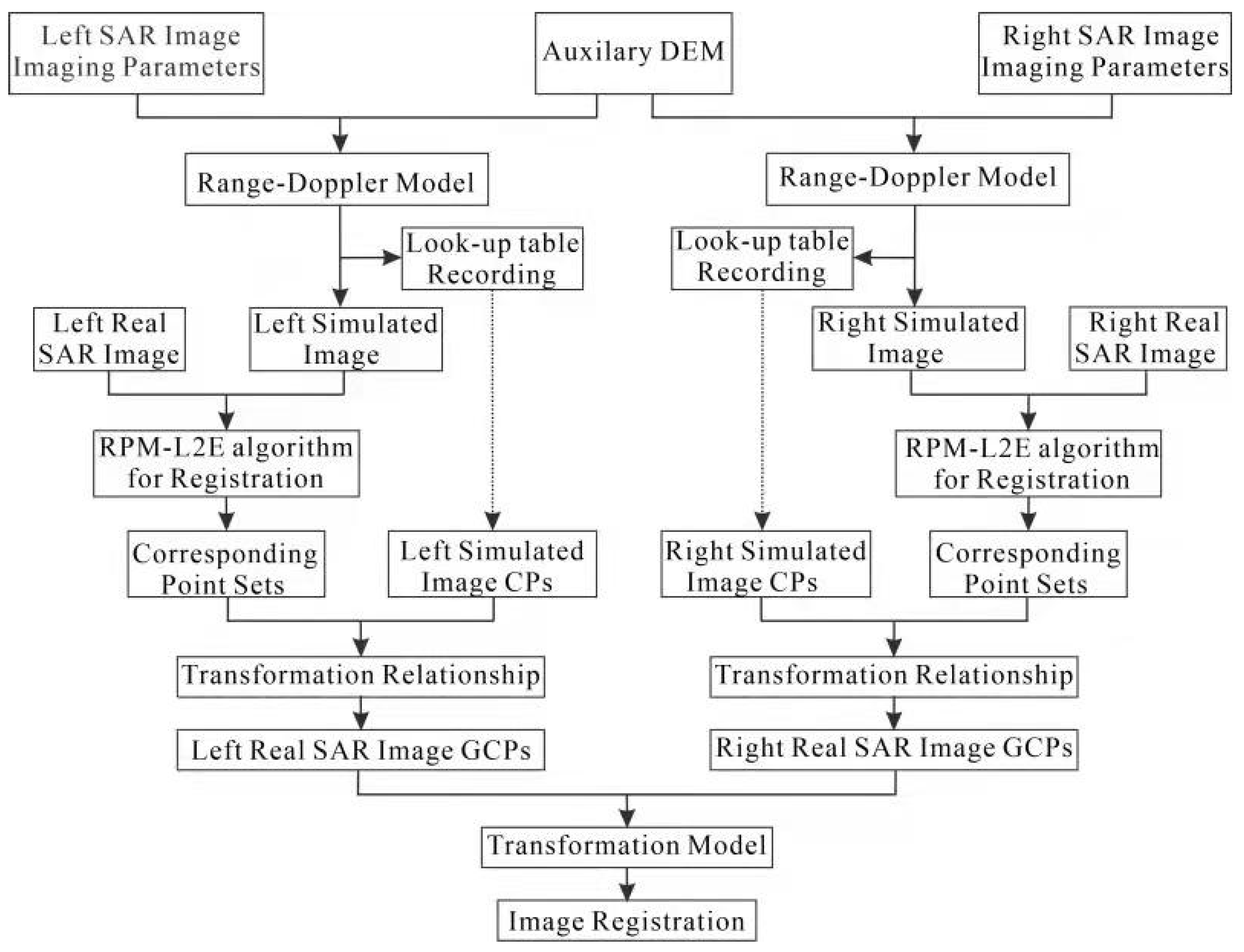
3. Methodology
3.1. SAR Image Simulation
3.1.1. SAR Image Geometric Simulation
3.1.2. SAR Image Grayscale Simulation
3.1.3. DEM Interpolation
3.2. Transformation of the Image Coordinate Relation
4. The Results of the Experiments and Their Analysis
4.1. Experimental Data
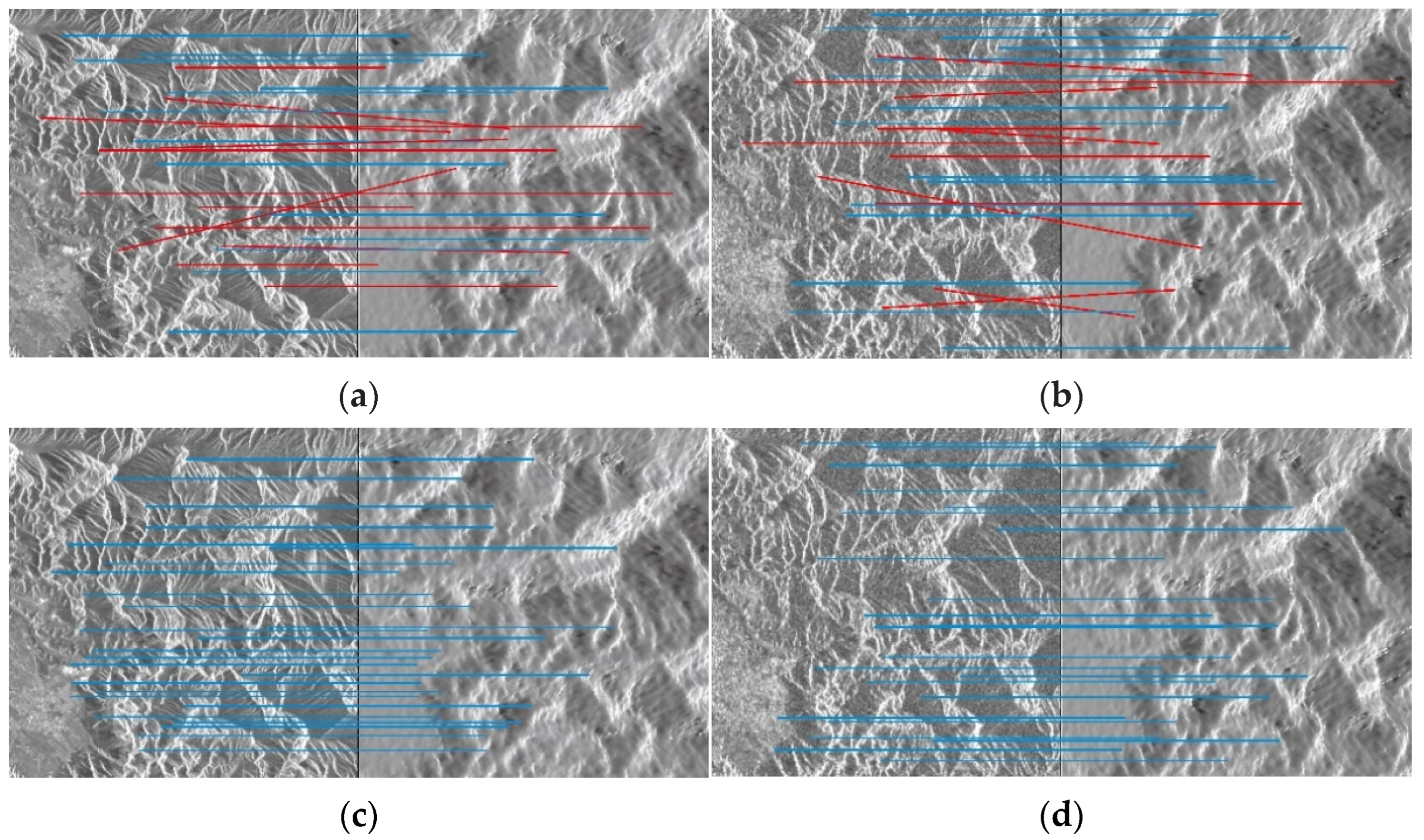
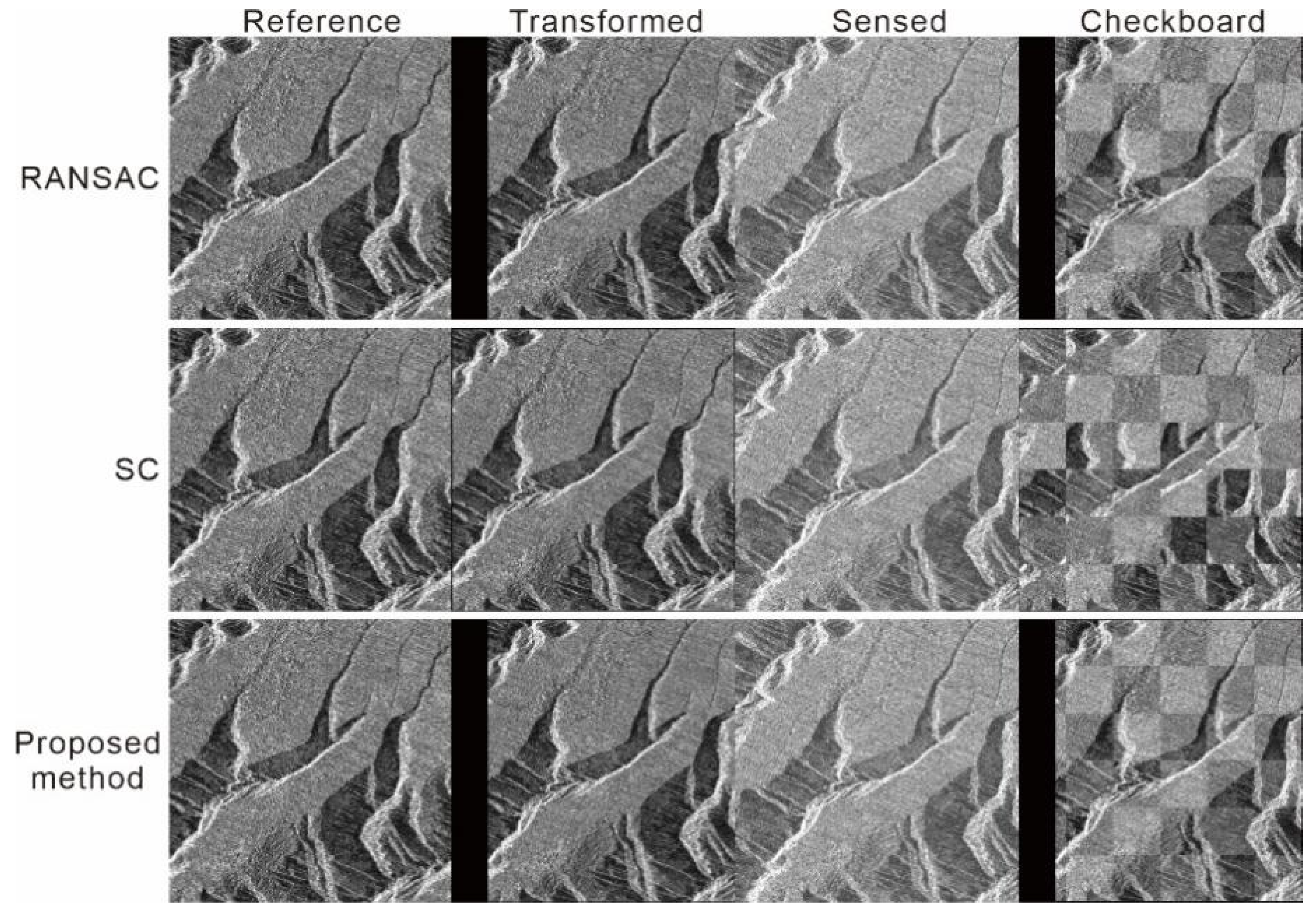
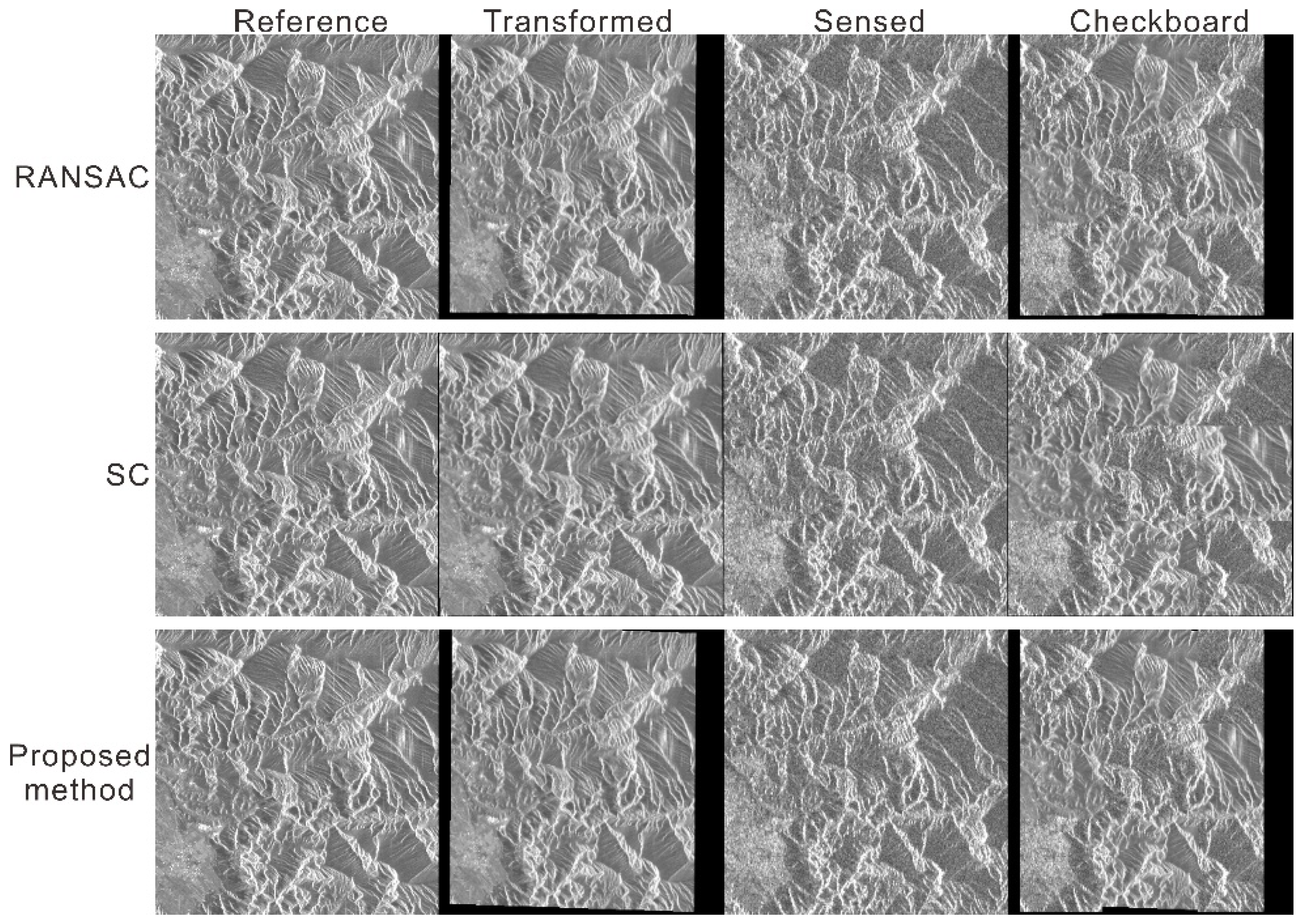
4.2. The Results of the Experiments
- Registration results between SAR images
5. Conclusions
Author Contributions
Funding
Institutional Review Board Statement
Informed Consent Statement
Data Availability Statement
Conflicts of Interest
References
- Price, F.M.; Arnesen, T.; Gløersen, E.; Metzger, M.J. Mapping Mountain Areas: Learning from Global, European and Norwegian Perspectives. J. Mt. Sci. 2019, 16, 1–15. [Google Scholar] [CrossRef] [Green Version]
- Li, C.; Criss, R.E.; Fu, Z.; Long, J.; Tan, Q. Evolution Characteristics and Displacement Forecasting Model of Landslides with Stair-Step Sliding Surface Along the Xiangxi River, Three Gorges Reservoir Region, China. Eng. Geol. 2021, 283, 105961. [Google Scholar] [CrossRef]
- Li, C.; Long, J.; Liu, Y.; Li, Q.; Liu, W.; Feng, P.; Li, B.; Xian, J. Mechanism analysis and partition characteristics of a recent highway landslide in Southwest China based on a 3D multi-point deformation monitoring system. Landslides 2021, 18, 2895–2906. [Google Scholar] [CrossRef]
- Zhang, G.-P.; Xu, J.; Bi, B.-G. Relations of Landslide and Debris Flow Hazards to Environmental Factors. Yingyong Shengtai Xuebao 2009, 20, 653–658. [Google Scholar]
- Deuskar, C.; Baker, J.L.; Mason, D. East Asia’s Changing Urban Landscape: Measuring a Decade of Spatial Growth; World Bank Publications: Washington, DC, USA, 2015. [Google Scholar]
- Li, C.; Wang, R.; Gu, D.; Wang, J.; Chen, X.; Zhou, J.; Liu, Z. Temperature and ice form effects on mechanical behaviors of ice-richmoraine soil of Tianmo valley nearby the Sichuan-Tibet Railway. Eng. Geol. 2022, 305, 106713. [Google Scholar] [CrossRef]
- Auh, S.-C.; Lee, S.-B. Analysis of the Effect of Tropospheric Delay on Orthometric Height Determination at High Mountain. KSCE J. Civ. Eng. 2018, 22, 4573–4579. [Google Scholar] [CrossRef]
- Katarzyna, C.; Cienkosz, D.; Apollo, M.; Borowski, Ł.; Lewinska, P.; Santos, C.A.G.; Eborka, K.; Kulshreshtha, S.; Romero-Andrade, R.; Sedeek, A. Challenges Related to the Determination of Altitudes of Mountain Peaks Presented on Cartographic Sources. Geod. Vestn. 2022, 66, 49–59. [Google Scholar]
- Langbein, J.; Svarc, J.L. Evaluation of Temporally Correlated Noise in Global Navigation Satellite System Time Series: Geodetic Monument Performance. J. Geophys. Res. Solid Earth 2019, 124, 925–942. [Google Scholar] [CrossRef] [Green Version]
- Feifei, Q.; Lu, Z.; Zhang, Q.; Bawden, G.W.; Kim, J.; Zhao, C.; Qu, W. Mapping Ground Deformation over Houston-Galveston, Texas Using Multi-Temporal Insar. Remote Sens. Environ. 2015, 169, 290–306. [Google Scholar]
- Zhou, C.; Gong, H.; Chen, B.; Li, X.; Li, J.; Wang, X.; Gao, M.; Si, Y.; Guo, L.; Shi, M. Quantifying the Contribution of Multiple Factors to Land Subsidence in the Beijing Plain, China with Machine Learning Technology. Geomorphology 2019, 335, 48–61. [Google Scholar] [CrossRef]
- Chen, B.; Gong, H.; Chen, Y.; Li, X.; Zhou, C.; Lei, K.; Zhu, L.; Duan, L.; Zhao, X. Land subsidence and its relation with groundwater aquifers in Beijing Plain of China. Sci. Total Environ. 2020, 735, 139111. [Google Scholar] [CrossRef]
- Krieger, G. Mimo-Sar: Opportunities and Pitfalls. IEEE Trans. Geosci. Remote Sens. 2013, 52, 2628–2645. [Google Scholar] [CrossRef] [Green Version]
- Curlander, J.C.; Mcdonough, R.N. Synthetic Aperture Radar: Systems and Signal Processing; Wiley: Hoboken, NJ, USA, 1991. [Google Scholar]
- Amelung, F.; Galloway, D.; Bell, J.W.; Zebker, H.A.; Laczniak, R.J. Sensing the ups and downs of Las Vegas: InSAR reveals structural control of land subsidence and aquifer-system deformation. Geology 1999, 27, 483–486. [Google Scholar] [CrossRef]
- Bawden, G.W.; Thatcher, W.; Stein, R.S.; Hudnut, K.W.; Peltzer, G. Tectonic contraction across Los Angeles after removal of groundwater pumping effects. Nature 2001, 412, 812–815. [Google Scholar] [CrossRef] [PubMed]
- Buckley, S.M.; Rosen, P.A.; Hensley, S.; Tapley, B. Land subsidence in Houston, Texas, measured by radar interferometry and constrained by extensometers. J. Geophys. Res. Earth Surf. 2003, 108, 2542. [Google Scholar] [CrossRef]
- Xun, Z.; Zhao, C.; Kang, Y.; Liu, X.; Liu, Y.; Du, C. Automatic Extraction of Potential Landslides by Integrating an Optical Remote Sensing Image with an InSAR-Derived Deformation Map. Remote Sens. 2022, 14, 2669. [Google Scholar] [CrossRef]
- Strozzi, T.; Wegmuller, U.; Tosi, L.; Bitelli, G.; Spreckels, V. Land Subsidence Monitoring with Differential Sar Interferometry. Photogramm. Eng. Remote Sens. 2001, 67, 1261–1270. [Google Scholar]
- Xing, M.; Bao, Z.; Li, Z.; Wang, T. Advancement of Radar Imaging Algorithm. Beijing, China; Publishing House of Electronics Industry: Beijing, China, 2014. [Google Scholar]
- Dai, X.; Khorram, S. The Effects of Image Misregistration on the Accuracy of Remotely Sensed Change Detection. IEEE Trans. Geosci. Remote Sens. 1998, 36, 1566–1577. [Google Scholar] [CrossRef] [Green Version]
- Petillot, I.; Trouve, E.; Bolon, P.; Julea, A.; Yan, Y.; Gay, M.; Vanpe, J.-M. Radar-Coding and Geocoding Lookup Tables for the Fusion of GIS and SAR Data in Mountain Areas. IEEE Geosci. Remote Sens. Lett. 2009, 7, 309–313. [Google Scholar] [CrossRef]
- Zitová, B.; Flusser, J. Image registration methods: A survey. Image Vis. Comput. 2003, 21, 977–1000. [Google Scholar] [CrossRef] [Green Version]
- Brown, L.G. A survey of image registration techniques. ACM Comput. Surv. 1992, 24, 325–376. [Google Scholar] [CrossRef]
- Sedaghat, A.; Mokhtarzade, M.; Ebadi, H. Uniform Robust Scale-Invariant Feature Matching for Optical Remote Sensing Images. IEEE Trans. Geosci. Remote Sens. 2011, 49, 4516–4527. [Google Scholar] [CrossRef]
- Mikolajczyk, K.; Schmid, C. A Performance Evaluation of Local Descriptors. IEEE Trans. Pattern Anal. Mach. Intell. 2005, 27, 1615–1630. [Google Scholar] [CrossRef] [PubMed] [Green Version]
- Lowe, D.G. Distinctive Image Features from Scale-Invariant Keypoints. Int. J. Comput. Vis. 2004, 60, 91–110. [Google Scholar] [CrossRef]
- Yue, H.; Hanssen, R.; Kianicka, J.; Marinkovic, P.; Ketelaar, G. Sensitivity of topography on insar data coregistration. In Proceedings of the 2004 Envisat & ERS Symposium, Salzburg, Austria, 6–10 September 2004. [Google Scholar]
- Curlander, J.C. Location of Spaceborne Sar Imagery. IEEE Trans. Geosci. Remote Sens. 1982, GE-20, 359–364. [Google Scholar] [CrossRef]
- Chen, E. Study on Ortho-Rectification Methodology of Space-Borne Synthetic Aperture Radar Imagery; Academy of Forestry: Beijing, China, 2004. [Google Scholar]
- Ma, J.; Qiu, W.; Zhao, J.; Ma, Y.; Yuille, A.L.; Tu, Z. Robust L2E Estimation of Transformation for Non-Rigid Registration. IEEE Trans. Signal Process. 2015, 63, 1115–1129. [Google Scholar] [CrossRef]
- Scott, D.W. Parametric Statistical Modeling by Minimum Integrated Square Error. Technometrics 2001, 43, 274–285. [Google Scholar] [CrossRef]
- Basu, A.; Harris, I.R.; Hjort, N.L.; Jones, M.C. Robust and efficient estimation by minimising a density power divergence. Biometrika 1998, 85, 549–559. [Google Scholar] [CrossRef] [Green Version]
- Chui, H.; Rangarajan, A. A new point matching algorithm for non-rigid registration. Comput. Vis. Image Underst. 2003, 89, 114–141. [Google Scholar] [CrossRef]
- Belongie, S.; Malik, J.; Puzicha, J. Shape Matching and Object Recognition Using Shape Contexts. IEEE Trans. Pattern Anal. Mach. Intell. 2002, 24, 509–522. [Google Scholar] [CrossRef] [Green Version]
- Yuille, A.L.; Grzywacz, N.M. A Mathematical Analysis of the Motion Coherence Theory. Int. J. Comput. Vis. 1989, 3, 155–175. [Google Scholar] [CrossRef]
- Aronszajn, N. Theory of Reproducing Kernels. Trans. Am. Math. Soc. 1950, 68, 337–404. [Google Scholar] [CrossRef]
- Micchelli, C.A.; Pontil, M. On Learning Vector-Valued Functions. Neural Comput. 2005, 17, 177–204. [Google Scholar] [CrossRef]
- Zhao, J.; Ma, J.; Tian, J.; Ma, J.; Zhang, D. A robust method for vector field learning with application to mismatch removing. In Proceedings of the CVPR 2011, Colorado Springs, CO, USA, 20–25 June 2011; pp. 2977–2984. [Google Scholar] [CrossRef]
- Rifkin, R.; Yeo, G.; Poggio, T. Regularized Least-Squares Classification. Acta Electron. Sin. 2003, 290, 131–153. [Google Scholar]
- Muhleman, D.O. Symposium on Radar and Radiometric Observations of Venus During the 1962 Conjunction: Radar Scattering from Venus and the Moon. ASTRON J. 1964, 69, 34–41. [Google Scholar] [CrossRef]
- Fischler, M.A.; Bolles, R.C. Random Sample Consensus: A Paradigm for Model Fitting with Applications to Image Analysis and Automated Cartography. Commun. ACM 1981, 24, 381–395. [Google Scholar] [CrossRef]


| SAR Images | Sensor | Spatial Resolution | Incident Angle | Elevation Range | Size | Date of Acquisition | Location of Acqusition | |
|---|---|---|---|---|---|---|---|---|
| Experiment 1 | Ref. image | TerraSAR | 3 m | 30.99° | 600 m ~800 m | 600 × 600 | 11 October 2011 | Yuncheng |
| Sen. image | TerraSAR | 3 m | 30.99° | 600 m ~800 m | 600 × 600 | 2 November 2011 | Yuncheng | |
| Experiment 2 | Ref. image | TerraSAR | 1.5 m | 41.8° | 1800 m ~2100 m | 300 × 300 | 24 January 2016 | Heifangtai |
| Sen. image | Sentinel | 15 m | 33.84° | 1800 m ~2100 m | 300 × 300 | 13 April 2017 | Heifangtai | |
| SAR Images | Method | Number of Matching Points | |||
|---|---|---|---|---|---|
| Reference Image | Correct Match | Reference Image | Correct Match | ||
| Experiment 1 | SIFT | 15 | 10 | 16 | 9 |
| RPM-L2E | 20 | 20 | 16 | 16 | |
| Experiment 2 | SIFT | 26 | 13 | 26 | 15 |
| RPM-L2E | 26 | 26 | 23 | 23 | |
| SAR Images | Methods | RMSE/Pixel | MI |
|---|---|---|---|
| Experiment 1 | RANSAC | 0.028 | 0.48 |
| SC | 0.047 | 0.097 | |
| Our approach | 0.024 | 0.54 | |
| Experiment 2 | RANSAC | 0.036 | 0.64 |
| SC | 0.071 | 0.020 | |
| Our approach | 0.035 | 0.66 |
Publisher’s Note: MDPI stays neutral with regard to jurisdictional claims in published maps and institutional affiliations. |
© 2022 by the authors. Licensee MDPI, Basel, Switzerland. This article is an open access article distributed under the terms and conditions of the Creative Commons Attribution (CC BY) license (https://creativecommons.org/licenses/by/4.0/).
Share and Cite
Zhang, S.; Sui, L.; Zhou, R.; Xun, Z.; Du, C.; Guo, X. Mountainous SAR Image Registration Using Image Simulation and an L2E Robust Estimator. Sustainability 2022, 14, 9315. https://doi.org/10.3390/su14159315
Zhang S, Sui L, Zhou R, Xun Z, Du C, Guo X. Mountainous SAR Image Registration Using Image Simulation and an L2E Robust Estimator. Sustainability. 2022; 14(15):9315. https://doi.org/10.3390/su14159315
Chicago/Turabian StyleZhang, Shuang, Lichun Sui, Rongrong Zhou, Zhangyuan Xun, Chengyan Du, and Xiao Guo. 2022. "Mountainous SAR Image Registration Using Image Simulation and an L2E Robust Estimator" Sustainability 14, no. 15: 9315. https://doi.org/10.3390/su14159315
APA StyleZhang, S., Sui, L., Zhou, R., Xun, Z., Du, C., & Guo, X. (2022). Mountainous SAR Image Registration Using Image Simulation and an L2E Robust Estimator. Sustainability, 14(15), 9315. https://doi.org/10.3390/su14159315