Abstract
Demand forecasting is a crucial component of demand management. While shortening the forecasting horizon allows for more recent data and less uncertainty, this frequently means lower data aggregation levels and a more significant data sparsity. Furthermore, sparse demand data usually result in lumpy or intermittent demand patterns with irregular demand intervals. The usual statistical and machine learning models fail to provide good forecasts in such scenarios. Our research confirms that competitive demand forecasts can be obtained through two models: predicting the demand occurrence and estimating the demand size. We analyze the usage of local and global machine learning models for both cases and compare the results against baseline methods. Finally, we propose a novel evaluation criterion for the performance of lumpy and intermittent demand forecasting models. Our research shows that global classification models are the best choice when predicting demand event occurrence. We achieved the best results using the simple exponential smoothing forecast to predict demand sizes. We tested our approach on real-world data made up of 516 time series corresponding to the daily demand, over three years, of a European original automotive equipment manufacturer.
1. Introduction
Demand forecasting is a critical component of supply chain management, directly affecting production planning and order fulfillment. Accurate forecasts have an impact across the whole supply chain and affect manufacturing plant organization: operational and strategic decisions are made regarding resources (the allocation and scheduling of raw material and tooling), workers (scheduling, training, promotions, and hiring), manufactured products (market share increase and production diversification), and logistics for deliveries.
To issue accurate forecasts, we have to consider demand characteristics (Kim et al. [1] and Moon et al. [2]). Multiple demand characterizations have been proposed (Williams [3] and Johnston et al. [4]), and one of the most influential is the characterization proposed by Syntetos et al. [5], which divides demand patterns into four quadrants based on the inter-demand interval and the coefficient of variation. The four demand types are smooth (regular demand occurrence and low demand quantity variation), erratic (regular demand occurrence and high demand quantity variation), intermittent (irregular demand occurrence and low demand quantity variation), and lumpy (irregular demand occurrence and high demand quantity variation). Intermittent and lumpy demand problems are considered among the most challenging demand forecasting problems (Amin-Naseri et al. [6] and Mukhopadhyay et al. [7]). Both present infrequent demand arrivals with many zero-demand periods; these factors pose an additional challenge to accurate demand quantity estimation. Demand quantity estimation is harder for lumpy demand since it also presents variable demand sizes (Petropoulos et al. [8] and Bartezzaghi et al. [9]). Nevertheless, intermittent demand items account for considerable proportions of any organization’s stock value (Babai et al. [10]). Furthermore, for a use case described by Johnston et al. [11], it was found that 75% of items had a lumpy demand and accounted for 40% of the company’s revenue and 60% of stock investment. Along this line, Amin-Naseri et al. [6] cite multiple authors who observe that lumpy patterns are widespread, especially in organizations that hold many spare parts, such as the process, aviation, and automotive industries, as well as companies dealing with telecommunication systems, large compressors, and other examples.
Increasing industry automation, digitalization, and information sharing (e.g., through electronic data interchange software), fomented by national and regional initiatives (Davies [12], Glaser [13], and Yang et al. [14]), accelerates the data and information flow within an organization, enabling greater agility. Therefore, it is critical to develop demand forecasting models capable of providing forecasts at a low granularity level to achieve greater agility in supply chain management. Such models enable short forecasting horizons and provide insights at a significant level of detail, allowing organizations to foresee and react to changes quickly. However, while these forecasting models benefit from the most recent data available (which helps enhance the forecast’s accuracy), the low granularity level frequently requires dealing with irregular demand patterns (Syntetos et al. [15]).
Given the variety of demand types, researchers have proposed multiple approaches to providing accurate demand forecasts. While smooth and erratic demand patterns achieve good results using regression models, intermittent and lumpy demand require specialized models that consider demand occurrence. Statistical, machine learning, and hybrid models have been developed to that end. The increase in industry digitalization enables the timely collection of data relevant to demand forecasts. Data availability is critical for developing machine learning models, which sometimes achieve the best results.
To deal with intermittent demand, Croston [16] proposed a forecasting model that provides separate estimates for demand occurrence and demand quantity. Since then, much work has followed this direction. The measurement of intermittent and lumpy model performance has also been the subject of extensive research. Many authors agree that we require regression accuracy and inventory metrics. Furthermore, there is increasing agreement that regression metrics alone, used for smooth and erratic demand, do not help measure intermittent and lumpy demand since they fail to weigh zero-demand periods. Inventory metrics suffer the same bias while providing a perspective on how much time products stay in stock.
Croston’s intuition in separating demand occurrence from demand sizes was valuable. While many authors followed this intuition, we found that in the reviewed literature, no author fully considered demand forecasting as a compound problem that required separate models and metrics. We propose reframing demand forecasting as a two-phase problem that requires (i) a classification model to predict demand occurrence and (ii) a regression model to predict demand sizes. Classification can be omitted for smooth and erratic demand patterns since demand (almost) always occurs. In those cases, using only a regression model provides good demand forecasts (Brühl et al. [17], Wang et al. [18], Sharma et al. [19], Gao et al. [20], Salinas et al. [21], and Bandara et al. [22]). For intermittent and erratic demand patterns, using separate models for classification and regression provides at least two benefits. First, separate models allow optimization for different objectives. Second, each problem has adequate metrics, and the cause of performance or under-performance can be clearly understood and addressed.
In this research, we propose:
- Decoupling the demand forecasting problem into two separate problems: classification (demand occurrence) and regression (demand quantity estimation);
- Using four measurements to assess demand forecast performance: (i) the area under the receiver operating characteristic curve (AUC ROC) (Bradley [23]) to assess demand occurrence, (ii) two variations of the mean absolute scaled error (MASE) (Hyndman et al. [24]) to assess demand quantity forecasts, and (iii) stock-keeping-oriented prediction error cost (SPEC), proposed by Martin et al. [25] as an inventory metric;
- A new demand classification schema based on the existing literature and our research findings.
We compared the statistical methods proposed by Croston [16], Syntetos et al. [26], and Teunter et al. [27]; the hybrid models developed by Nasiri Pour et al. [28] and Willemain et al. [29]; the ADIDA forecasting method introduced by Nikolopoulos et al. [30]; an extreme learning machine (ELM) model proposed by Lolli et al. [31]; and the VZadj model described by Hasni et al. [32]. We measured their performance using classification, regression, and inventory metrics. We also developed a compound model that outperforms the ones listed above.
We performed our research on a dataset consisting of 516 time series of intermittent and lumpy demand at a daily aggregation level, corresponding to the demand of European manufacturing companies related to the automotive industry.
The rest of this paper is structured as follows: Section 2 presents related work, Section 3 describes our approach to demand forecasting, with a particular focus on intermittent and lumpy demand, Section 4 describes the features we created for each forecasting model, as well as how we built and evaluated them, and Section 5 describes the experiments we performed and the results obtained. In Section 6, we provide our conclusions and outline future work.
2. Related Work
2.1. Demand Characterization
Many authors have tried to characterize demand to support stock management, determine material planning strategies, and provide cues to decide which forecasting model is most appropriate for each case. A common practice is to classify products into three categories (ABC) according to their cost–volume share: A usually includes items with a large cost–volume share, B is for items with a moderate cost–volume share, and C is for items with a low cost–volume share (Flores et al. [33]). Another three categories are proposed by the FSN approach, which divides products according to their demand velocity into the fast-moving, slow-moving, and non-moving categories (Mitra et al. [34]). XYZ categorization divides items according to their fluctuations in consumption: X for items with almost constant consumption, Y for items with consumption fluctuations (due to trends or seasonality), and Z for items with irregular demand (Scholz-Reiter et al. [35]). Botter et al. [36] mention the VED approach, where products are divided into a different set of categories: vital parts (that cause high losses if not present in stock), essential parts (that cause moderate losses if not available in stock), and desirable parts (that cause minor disruptions to the manufacturing process if not present in stock). ABC categorization has been used jointly with several of the aforementioned categorization schemes. For example, Nallusamy et al. [37] reported using a mixed approach combining the ABC and FSN analyses, while Scholtz et al. [35] combined the ABC and XYZ analyses. Croston [16] proposed another approach that assessed demand based on demand size and inter-demand intervals. Williams [3] considered the variance in the number and size of orders given a particular lead time, classifying items into five categories based on high/low demand sporadicity and size. Based on the author’s empirical findings regarding demand intermittence, a particular category was created for products with a highly sporadic demand occurrence and high demand size variance. Eaves et al. [38] found that the classification schema proposed by Williams did not provide the means to distinguish continuous demand solely based on transaction variability. They proposed dividing demand into five categories based on lead time variability, transaction rate variability, and demand size variability.
Equation (1): ADI stands for average demand interval.
Equation (2): CV stands for coefficient of variation. It is computed over non-zero demand occurrences (Syntetos et al. [39]).
Johnston et al. [4] introduced the concept of the average demand interval (ADI, see Equation (1)), which was complemented by Syntetos et al. [5], who introduced the coefficient of variation (CV, see Equation (2)). Both concepts allow us to divide demand into quadrants, i.e., the smooth, erratic, intermittent, and lumpy demand types (see Figure 1). Smooth and erratic demand present regular demand; smooth demand has little variability in demand sizes, while this variability is strong for erratic demands. Intermittent and lumpy demand present irregular demand intervals over time. Intermittent demand has little variability in demand sizes, unlike lumpy demand, which has a greater demand size variability. Thresholds were set based on empirical findings regarding where the methods proposed by Croston [16] and Syntetos et al. [39,40] performed best.
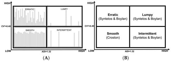
Figure 1.
Demand pattern classification. (A) depicts different demand patterns, while (B) shows the classification proposed by Syntetos et al. [5] based on empirical findings.
In this paper, we use the term continuous demand to refer to smooth and erratic demand (both of which display regular demand occurrence) and irregular demand or sparse demand for intermittent and lumpy demand (both of which display irregular or infrequent demand occurrence).
2.2. Forecasting Sparse Demand
In order to mitigate lumpiness, four traditional strategies are frequently used in manufacturing: (a) the use of fixed additional capacity to handle peaks, (b) additional inventories, (c) order rejection during high-demand periods, and (d) temporary increases in manufacturing capacity (e.g., using subcontractors, overtime, or introducing additional shifts) (Arzi et al. [41]). However, accurate forecasts can reduce the need for such approaches, protect the firm’s reputation (e.g., by not rejecting consumer orders), and reduce costs (e.g., ensuring enough planned capacity to meet the expected demand).
Forecasting irregular demand is considered a challenging task since it requires considering irregular demand occurrence in addition to the demand size forecast. Box–Jenkins approaches, frequently used for regular time series forecasting, are considered useless in the context of irregular demand (Wallström et al. [42]) since it is challenging to estimate trends and seasonality given the high proportion of zeros. Therefore, researchers developed specialized models to tackle this particular type of demand.
2.3. Demand Forecasting Models
Forecasting irregular demand is considered a challenging task since, in addition to the demand size forecast, it requires taking into account irregular demand occurrence. A seminal work regarding intermittent demand forecasting was developed by Croston [16], who identified exponential smoothing as inadequate for estimating demand when the mean demand interval between two transactions is greater than two time periods. He proposed a method to estimate the expected interval between transactions and the expected demand size (Equation (3)). Assuming that successive demand intervals and sizes are independent, the inter-demand intervals follow a geometric distribution, and the demand sizes follow a normal distribution. Shenstone et al. [43] showed that Croston’s method was not consistent with intermittent demand properties, but its results still outperformed conventional methods. Many researchers followed Croston’s approach, either by enhancing this method or proposing similar ones.
Equation (3): Croston’s formula [16] for irregular demand estimation, where a is the demand level, p is periodicity, d refers to demand observations, q is previous demand occurrence, and α represents a smoothing constant.
Syntetos et al. [26] proposed a slight modification to Croston’s method, known as the Syntetos–Boylan approximation (SBA), in order to avoid a positive correlation between the forecasted demand size and the smoothing constant (Equation (4)). Levén et al. [44] suggested computing a new demand rate every time demand takes place, considering a maximum of one time per time bucket. Teunter et al. [45] considered computing a demand probability for each period and updating the demand quantity forecast only when demand takes place (Equation (5)). In a similar line of research, Vasumathi et al. [46] adapted Croston’s method by considering the average of the last two demands. Prestwich et al. [47] proposed a hybrid of Croston’s method and Bayesian inference to consider items’ obsolescence. Türkmen et al. [48] considered intermittent demand forecasting models as instances of renewal processes and extended Croston’s method for a probabilistic forecast. Furthermore, they envisioned that Croston-type methods could be replaced by recurrent neural networks. Chua et al. [49] developed an algorithm that estimated future demand occurrence based on three time series: non-zero-demand periods, inter-arrival periods between demand occurrences, and periods spanning between two demand occurrences. They estimated demand size with a simple moving average.
Equation (4): Syntetos et al. [26] proposed the Syntetos–Boylan Approximation as an adjusted version of Croston’s [16] forecast formula.
Equation (5): The Teunter, Syntetos, and Babai formula [45] for irregular demand estimation, where a is the demand level, p is the probability of demand occurrence, d refers to demand observations, q is previous demand occurrence, and α represents a smoothing constant.
Wright [50] developed linear exponential smoothing, an adaptation of Holt’s double exponential smoothing model that considers variable reporting frequency and irregularities in time spacing to compute and update a trend line with exponential smoothing. Altay et al. [51] demonstrated that this method helps forecast intermittent demand where the trend is present. Sani et al. [52] and Ghobbar et al. [53] found that averaging methods can provide acceptable performance in some cases, despite demand intermittency. Chatfield et al. [54] suggested using a zero-demand model for highly lumpy demand, where the holding cost is much higher than the shortage cost. Gutierrez et al. [55] proposed forecasting lumpy demand with a three-layer multilayer perceptron (MLP) (Rosenblatt [56]), considering only two inputs: the demand of the immediately preceding period and the number of periods separating the last two non-zero-demand transactions. Along the same line, Lolli et al. [31] considered using ELM (Huang et al. [57]) and training the model based on three input features: (a) the demand size for the previous time period, (b) the number of periods separating the last two non-zero-demand transactions considering the immediately preceding period, and (c) the cumulative number of successive periods with zero demand.
Some researchers proposed performing data aggregation to achieve smooth time series to cope with event sparsity. Much research was performed on the effect of aggregation on regular time series (Hotta et al. [58], Souza et al. [59], Athanasopoulos et al. [60], Rostami-Tabar et al. [61,62], Petropoulos et al. [8], and Kourentzes et al. [63]), showing that higher aggregation improves forecast results. One such approach is the aggregate–disaggregate intermittent demand approach (ADIDA) (Nikolopoulos et al. [30]), which is a three-stage process: (i) perform time-series aggregation (either overlapping or non-overlapping aggregation), (ii) forecast the next time series value over the aggregated time series, and (iii) disaggregate the forecasted value to the original aggregation level.
Following Croston’s intuition [16], some researchers developed separate models to forecast demand occurrence and demand size. Willemain et al. [29] proposed to model demand occurrence as a Markov process and forecast demand size by randomly sampling past demand sizes and eventually jittering them to account for not-yet-seen values. Hua et al. [64] followed a similar approach, attributing demand occurrence to autocorrelation or explanatory variables. If they attributed demand occurrence to autocorrelation, they predicted it based on Markov processes. Otherwise, they used a logistic regression model. Nasiri Pour et al. [28] developed a hybrid approach, forecasting demand occurrence with a neural network (see Figure 2) while they estimated demand size with exponential smoothing. The neural network they proposed considered four input variables: (a) the demand size at the end of the preceding period, (b) the number of periods between the last two demand occurrences, (c) the number of periods between the target period and the last demand occurrence, and (d) the number of periods between target period and first immediately preceding zero-demand period. The authors considered demand to not occur if the network forecasted a zero value and considered demand to take place if the predicted value was greater than zero.
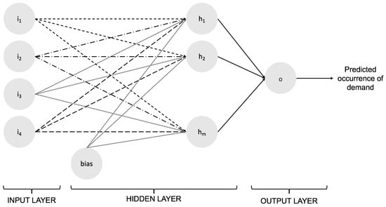
Figure 2.
MLP for the hybrid approach proposed by Nasiri Pour et al. [28]. The inputs to the model are the demand size at the end of the preceding period, the number of periods between the last two demand occurrences, the number of periods between the target period and the last demand occurrence, and the number of periods between the target period and the first immediately preceding zero-demand period.
Finally, Petropoulos et al. [65] developed an alternative perspective to the ADIDA framework (Nikolopoulos et al. [30]), aggregating time series in such a way that each time bucket contained a single demand occurrence. As a result, the transformed time series no longer presented intermittency, and it forecasted the time-varying number of periods when such demand would occur. Then, based on the mean values for the inter-demand interval and the coefficient of variation, demand size was estimated using Croston’s method, SBA, or simple exponential smoothing. A similar approach was described by Hasni et al. [32]. The authors proposed forecasting demand by repeatedly random sampling from the frequency histograms of past inter-demand intervals and demand sizes.
Forecasting Features
Bartezzaghi et al. [66] considered demand lumpiness as a consequence of different market characteristics, such as the numerousness and heterogeneity of customers, the frequency at which customers place the orders, the variety of customer requests (e.g., high customization in make-to-order settings (Verganti [67])), and the correlations between customer behavior). Lumpiness is also related to the granularity level at which demand is considered (e.g., visualizing demand at a client and product level vs. only at a product level or visualizing daily demand vs. monthly). Higher aggregation levels usually reduce the number of periods without demand, changing the demand pattern classification.
In the scientific literature related to the demand forecasting of intermittent and lumpy demand patterns, authors describe multiple characteristics and features relevant to demand occurrence forecasting. Among them, we find the average inter-demand interval size (Levén et al. [44]), the previous demand event occurrence (Gutierrez et al. [55]), the distribution of inter-demand interval sizes (Croston [16]), demand size (Nasiri Pour et al. [28]), demand shape distribution (Bartezzaghi et al. [68] and Zotteri [69]), the usage of early information generated by customers during the purchasing process (Verganti [67]), the presence of paydays, billing cycles, or holidays (Hyndman et al. [24]), demand event autocorrelation (Willemain et al. [70]), demand event correlation (products being complementary or alternate) (Arzi et al. [41]), and whether items may be purchased by the same supplier or shipped using the same transportation mode (Syntetos [71]).
We found that two techniques were applied to estimate demand size across all cases. The first one was exponential smoothing (and its variants), and it was applied across previous non-zero demand sizes (Nasiri Pour et al. [28]). The second one was the use of jittering on top of randomly sampled past demand sizes to account for yet-unseen values (Willemain et al. [29] and Hua et al. [64]). Altay et al. [51] described means to adjust demand size values based on the presence of trends in data.
On top of the above-mentioned approaches, two approaches used to reduce uncertainty regarding lumpiness can help create features: early sales and order overplanning (Verganti [67] and Bartezzaghi et al. [66]). The early sales approach considers information regarding actual orders received for future delivery, where future demand can be estimated given that some degree of correlation exists between the unknown and known portions of the demand. On the other hand, the order overplanning approach focuses on every customer instead of the overall demand. It, therefore, enables collecting and using information specific to each customer and their future needs.
2.4. Metrics
The measurement of forecasting models’ performance for lumpy and intermittent demand has been a subject of extensive research (Anderson [72]). Syntetos et al. [71] compared the performance of the Mean Signed Error, Wilcoxon Rank Sum Statistic, Mean Square Forecast Error, Relative Geometric Root Mean Square Error (RGRMSE), and Percentage of times Better metrics (PB). They concluded that the RGRMSE behaves well in the context of irregular demand. Teunter et al. [73] pointed out that the RGRMSE cannot be applied on a single item for zero or moving average forecasts (it would result in zero error). Hemeimat et al. [74] suggested using the tracking signal metric, which is calculated by dividing the most recent sum of forecast errors by the most recent estimate of the mean absolute deviation (MAD). Among many metrics, Hyndman et al. [24] suggested using the MASE for lumpy and intermittent demand to provide a scale-free assessment of the accuracy of demand size forecasts. Although traditional per-period forecasting metrics, such as the root mean squared error (RMSE), the mean squared error (MSE), the MAD, and the mean absolute percentage error (MAPE), were widely used in the literature regarding irregular demand, Teunter et al. [73] and Kourentzes [75] showed they were not adequate due to the high proportion of zeros. Prestwich et al. [76] proposed computing a modified version of the error measures that considered the mean of the underlying stochastic process instead of the point demand for each point in time. Finally, it is relevant to point out that two metrics were used in the M5 competition (Makridakis et al. [77]) to assess time series with respect to irregular sales: the root mean squared scaled error (RMSSE, introduced by Hyndman et al. [24]) and the weighted RMSSE. With these metrics, using a score that considers squared errors, result measurements optimize towards the mean. The weighted RMSSE variant allows for penalizing each time series error based on various criteria (e.g., item price). However, both metrics unevenly penalize products sold during the whole time period in contrast to those that are not.
Syntetos et al. [78] noted that regardless of the metrics used to estimate how accurate demand forecasts are, it is crucial to measure the impact of forecasts on stock-holding and service levels. Along this line, Wallström et al. [42] proposed two complementary metrics. The first one was the number of shortages, counting how many times the cumulated forecast error was over zero during the time interval of interest. The second one was periods in stock (PIS), defined as the number of periods the forecasted items spent in fictitious stock (or how many stock-out periods existed). More recently, Martin et al. [25] proposed the stock-keeping-oriented prediction error cost (SPEC), which considers, for each time step, whether demand forecasts translate into costs of opportunity or stock-keeping costs; the result is never both at the same time. We summarize the metrics adopted in relevant related works in Table 1.

Table 1.
Metrics identified in main related works we reviewed on the topic of lumpy and intermittent demand.
3. Reframing Demand Forecasting
3.1. A Classification of Existing Demand Forecasting Models for Lumpy and Intermittent Demand
From the models we presented in Section 2, we observe that certain patterns arose in how the demand forecasting problem for lumpy and intermittent demand was framed. We, therefore, classify the forecasting approaches into four categories:
- Type I: uses a single model to predict the expected demand size for a given time step.
- Type II: uses aggregation to remove demand intermittency and benefit from regular time series models to forecast demand.
- Type III: uses separate models to estimate whether demand will take place at a given point in time and the expected demand size.
- Type IV: uses separate models to estimate the demand interval and demand size.
We classify the models analyzed in the related works according to these four categories in Table 2.
Table 2.
Model types identified in main related works we reviewed on the topic of lumpy and intermittent demand.
3.2. Demand Characterization and Forecasting Models
Croston [16] developed the idea to consider two components for intermittent demand forecasts: demand occurrence and demand sizes. Syntetos et al. [5] considered these two components and developed an influential system of demand categorization, dividing demand into four types: smooth, erratic, intermittent, and lumpy, based on the coefficient of variation and the average demand interval. The need to separately address these two dimensions was further recognized by Nikolopoulos et al. [84].
Many authors followed Croston’s lead, developing separate models to estimate demand occurrence and demand size (e.g., Willemain et al. [29], Hua et al. [64], and Nasiri Pour et al. [28]), though none of them measured the performance of the demand occurrence component. We thus propose decoupling the demand forecasting problem into two sub-problems, each of which requires a separate model with separate features and metrics: (i) demand occurrence, addressed as a classification problem, and (ii) demand size estimation, addressed as a regression problem. Following the original work by Syntetos et al. [5] and the division mentioned above, we propose an alternative demand categorization schema. Considering demand occurrence and demand quantity forecasting as two different problems, we can divide demand into two types (see Figure 3). The first demand type is `R’, which refers to demand with regular demand event occurrence. Since demand (almost) always occurs in this case, estimating demand occurrence is rendered irrelevant and does not pose a challenge when developing a regression model to estimate demand size. The second demand type is ’C+R’, which refers to demand with an irregular occurrence. This second case benefits from models that consider both demand occurrence and demand size (see Section 2.3).
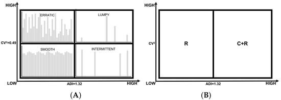
Figure 3.
Demand categorization schemas. On the right, (A) corresponds to the influential categorization developed by Syntetos et al. [5]. On the left, (B) proposes a new schema that only considers demand occurrence, dividing demand into two groups. ‘R’ denotes regular demand occurrence, where demand size can be predicted with a regression model. ‘C+R’ denotes irregular demand occurrence that requires a model to predict demand occurrence and a model to predict demand size.
In Figure 4, we present a demand forecasting model architecture and a flowchart describing how to build it and issue demand forecasts. Since the classification and regression models address different problems, we expect them to use different features to help achieve their goals. We described the aspects relevant to demand occurrence and demand size forecasting presented in the literature in Section 2.3. These can be used as the features of the classification and regression models.
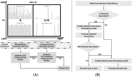
Figure 4.
Two-fold machine learning approach to demand forecasting. (A) shows a basic architecture for demand forecasting when reframing demand forecasting as classification and regression problems. (B) shows a flowchart with steps followed to create the demand forecasting models and issue demand forecasts.
An increasing body of research suggests that global machine learning time series models (models built with multiple time series) provide better results than local ones (models considering time series corresponding to a single product) (Bandara et al. [22] and Salinas et al. [21]). Furthermore, increased performance is observed even when training models with disparate time series that have different magnitudes or may not be related to each other (Laptev et al. [85] and Rožanec et al. [86]), although how to bound the maximum possible error in such models remains a topic of research. Given this insight, we conclude that dividing demand based on the coefficient of variation provides limited value and is no longer relevant to demand categorization.
We keep the cut-off value of ADI = 1.32 proposed by Syntetos et al. [5] as a reference. This cut-off value, jointly with the CV2, is accepted as a measure of whether a collection of observed demand is smooth, lumpy, intermittent, or erratic (Lowas III et al. [87]); it remains relevant for statistical methods. Nevertheless, we consider its relevance to blur with respect to different machine learning models. Its importance may be rendered irrelevant for global machine learning classification models that predict demand occurrence. By considering multiple items simultaneously, global models perceive a higher density of demand events and less irregularity than models developed with data regarding a single demand item. Simultaneously, the model can learn underlying patterns, which may be related to specific behaviors (e.g., deliveries that take place only on certain days). It is important to note that event scarcity usually results in imbalanced classification datasets, posing an additional challenge.
We present suggested metrics to assess each model, and the overall demand forecasting performance, in Section 3.3.
3.3. Metrics
Though several authors (e.g., [16,39,83]) considered separating demand occurrence and demand size when forecasting irregular demand, in the scientific literature we reviewed (see Table 1), we found that researchers measured them separately. We thus conclude that they did not consider demand occurrence and demand size forecast as entirely different problems.
Considering irregular demand forecasting only as a regression problem led to much research and discussion (presented in Section 2.4) on how to mitigate and integrate zero-demand occurrence to measure demand forecasting models’ performance adequately. In our research, we provide a different perspective. We adopt four metrics to assess the performance of demand forecasting models: (i) AUC ROC to measure how accurately the model forecasts demand occurrence, (ii) two variants of MASE to measure how accurately the model forecasts demand size, and (iii) SPEC to measure how the forecast impacts inventory. When measuring SPEC, we consider α1 = α2 = 0.5 since we have no empirical data that would support weighting α asymmetrically.
Equation (6): Stock-keeping-oriented Prediction Error Cost (SPEC).
AUC ROC is widely adopted as a classification metric and has many desirable properties, such as being threshold independent and invariant to a priori class probabilities. MASE has the desirable property of being scale-invariant. We consider two variants (namely MASEI and MASEII). Following the criteria in Wallström et al. [42], we compute MASEI for the time series that results from ignoring zero-demand values. By doing so, we assess how well the regression model performs against a näive forecast, assuming a perfect demand occurrence prediction. On the other hand, MASEII is computed for the time series that considers all points where demand either took place or is predicted according to the classification model. By doing so, we measure the impact of demand event occurrence misclassification on the demand size forecast. When the model predicting demand occurrence has perfect performance, (i) should equal (ii). Finally, we compute SPEC for the whole time series (considering zero and non-zero demand occurrences). This way, the metric measures the overall forecast impact on inventory, weighting stock-keeping, and opportunity costs.
4. Methodology
4.1. Business Understanding
Demand forecasting is critical to supply chain management since its outcomes directly affect the supply chain and manufacturing plant organizations. This research focuses on demand forecasting for a European original equipment manufacturer in the automotive industry. We explored providing demand forecasts for each material and client daily. Such forecasts enable highly detailed planning. From the forecasting perspective, accurate forecasts at a daily level can leverage the most recent information, which is lost at higher aggregation levels for non-overlapping aggregations. They also avoid imprecisions that result from higher-level forecast disaggregations. We tackled the demand forecasting problem as a modeling approach. In particular, we developed machine learning models that learn from past data to issue forecasts. In the following subsections, we provide a detailed insight into the steps we followed to create such predictive models.
4.2. Data Understanding
For this research, we used a dataset with three years of demand data extracted from enterprise resource planning software. We considered records that accounted for products shipped from manufacturing locations. For demand data, demand was registered on the day products shipped. The dataset comprised 516 time series corresponding to 279 materials and 149 clients. When categorized according to the schema proposed by Syntetos et al. [5], we found that 49 corresponded to a lumpy demand pattern and 467 to an intermittent demand pattern (see Figure 5). In Table 3 and Table 4, we provide summary statistics for the time series corresponding to each demand pattern. We found that demand occurrence for both sets of time series was highly infrequent, having a mean of one demand event in almost two months or more.
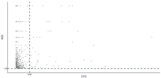
Figure 5.
The ADI-CV2 categorizations for the time series based on the classification proposed by Syntetos et al. [5].
Table 3.
Summary statistics for 49 lumpy demand time series.
Table 4.
Summary statistics for 467 intermittent demand time series.
4.3. Data Preparation, Feature Creation, and Modeling
We forecasted irregular demand with two separate models: a classification model to predict demand occurrence and a regression model to predict demand size. Though source data were the same for both, different features were required to address each model’s goals. Based on knowledge distilled from the literature, we created the features presented in Section 2.3 and some features of our own.
To model demand occurrence, we considered weekdays since last demand, the day of the week of the last demand occurrence, the day of the week for the target date, the mean of the inter-demand intervals, the mean of the last inter-demand intervals (across all products), and the skew and kurtosis of the demand size distributions, among other factors.
To model demand size, we considered, for each product, the size of the last demand, the average of the last three demand occurrences, the median value of past occurrences, the most frequent demand size value, and the exponential smoothing of past values, among other factors.
When computing feature values, we considered two forecasting horizons, namely fourteen and fifty-six days (Figure 6), to understand how the forecasting horizon size affects forecasts. The forecasting horizons were selected based on a business use case.
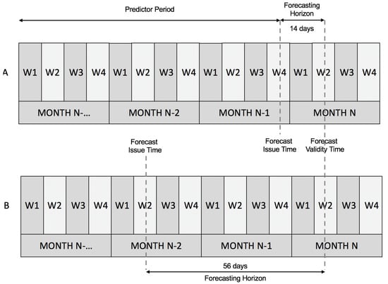
Figure 6.
We computed predictions for two forecasting horizons, i.e., 14 (A) and 56 (B) days, to test the sensitivity of predictions regarding demand occurrence and demand size to the forecasting horizon.
To forecast irregular demand, we compared nine methods described in the literature:
- Croston: Croston’s method [16] (see Equation (3)).
- SBA [26] (see Equation (4)).
- TSB [27] (see Equation (5)).
- MC+RAND: a hybrid model proposed by Willemain et al. [29]. Demand occurrence is estimated as a Markov process, while demand sizes are randomly sampled from previous occurrences.
- NN+SES: a hybrid model proposed by Nasiri Pour et al. [28]. Considers a NN model (see Figure 2) to forecast demand occurrence; demand size is computed by exponential smoothing over non-zero demand quantities in past periods. We used the following parameters for the NN: a maximum of 300 iterations, a constant learning rate of 0.01, and a hyperbolic tangent activation. Given that no description was given on whether scaling was applied to the dataset prior to training the network, we explored two models: without feature scaling (NNNS+SES) and with feature scaling (NNWS+SES).
- ADIDA forecasting method, proposed by Nikolopoulos et al. [30], which removes intermittence through aggregation and then disaggregates the forecast back to the original aggregation level.
- ELM: an ELM model as proposed by Lolli et al. [31]. We initialized the model with the following parameters: 15 hidden units, ReLU activation, a regularization factor of 0.1, and normal weight initialization. We trained two models: ELM(C1) (two models, trained per demand type) and ELM(C2) (global model, considering all the demand types).
- VZadj: a method proposed by Hasni et al. [32], considering only positive demands when the predicted lead-time demand was equal to the forecasting horizon considered.
We also developed models of our own. We created a CatBoost model (Prokhorenkova et al. [88]) to forecast demand occurrence and compare six models to forecast demand size: näive, most frequent value (MFV), moving average over last three demand periods (MA(3)), simple exponential smoothing (SES), random sampling from past values with jittering (RAND), and LightGBM regressor (ML). We used the LightGBM regression algorithm (Ke et al. [89]) because four of the top five time series forecasting models in the M5 competition were based on this algorithm (Makridakis et al. [77]).
CatBoost is an implementation of gradient-boosted decision trees. During training time, it sequentially builds a set of symmetric binary decision trees, ensuring that each new tree built reduces the loss compared to previous trees. The algorithm avoids one-hot-encoding categorical features by computing the frequency of the occurrence of particular values, reducing sparsity while enhancing computation times. CatBoost uses gradient descent to minimize a cost function, which informs how successful it is at meeting the classification goal. Since the dataset regarding demand occurrence was heavily imbalanced (less than 6% of instances corresponded to demand occurrence), we chose to optimize the model training with focal loss (Lin et al. [90]). Focal loss has the desirable property of asymmetric penalization of training samples, focusing on misclassified ones to improve the overall classification.
Our CatBoost classification model was built with a maximum depth of 2, 150 iterations, focal loss, and the AUC ROC evaluation metric. The LightGBM regressor was built with a maximum depth of 2, the RMSE objective, gradient-boosting decision tree boosting, 100 estimators, a learning rate of 0.1, and 31 tree leaves for base learners.
5. Experiments and Results
This section describes the experiments we conducted and assesses their results with the metrics described in Section 3.3. For the SPEC metric, we considered α1 and α2 equal to 0.5. We summarize our experiments in Table 5. In Table 6, we summarize the results obtained for our own models, while in Table 7, we compare the best-performing of our models against the models described in the scientific literature and described above (in Section 4.3).
Table 5.
Description of the reference models we evaluated for demand occurrence forecasting and demand size estimation.
Table 6.
Overall results obtained with the models we proposed, for both forecasting horizons. Best results are bolded, second-best results are displayed in italics.
Table 7.
Comparison of methods found in related works and three of the best models we created: C2R1-SES, C2R1-MFV, and C2R1-Näive. Our three models achieved the highest AUC ROC and showed competitive MASEI and MASEII values. C2R1-MFV achieved the best overall performance on the SPEC metric, while C2R1-Näive achieved the second-best result. Best results are bolded, and second-best results are presented in italics.
We adopted two forecasting horizons (fourteen and fifty-six days) to understand how sensitive the existing approaches were to forecast lead time. To evaluate the models, we used nested cross-validation (Stone [91]), which is frequently used to evaluate time-sensitive models. We tested our models by having them make predictions at the weekday level for six months of data. For the classification models, we measured AUC ROC, with prediction scores cut at a threshold of 0.5. The only exception to this was the model by Nasiri Pour et al. [28] since the authors explicitly stated that they considered any prediction above zero as an indication of demand occurrence.
We observed that although the approaches in the literature provided different means of estimating demand occurrence, their performance results were all close to 0.5 AUC ROC. Differences in performance were mainly driven by the method used to estimate demand size.
All the models we developed in our experiments strongly outperformed the models replicated from the literature. When considering AUC ROC, our models achieved scores of at least 0.94, almost doubling every model described in the literature. When considering regression metrics, our models displayed three to four times better MASEI and MASEII values and even larger differences regarding the SPEC metric for most models. The only exceptions were the ELM(C1) and ELM(C2) models, which achieved better MASE metrics but not competitive AUC ROC or SPEC values. These results confirm the importance of considering the demand forecasting of irregular demand patterns as two separate problems (demand occurrence and demand size), each with its features and optimized against its own set of metrics. The improvements in classification scores substantially impacted demand size and inventory metrics.
We obtained the best results with the CatBoost classifier trained over all instances, making no distinction between lumpy and intermittent demand. The model achieved a high classification AUC ROC score, reaching 0.97 for both the fourteen-day and fifty-six-day horizons. Among the regression models used to estimate demand size, we achieved the best results with SES, MFV, and Näive. SES outperformed every other model with respect to MASEI and MASEII, while MFV had the best median SPEC score and remained competitive on MASEI and MASEII values. The Näive variant achieved the second-best SPEC score while remaining competitive on MASE values.
When building the global classification model, we were interested in how much better it performed than models built using only lumpy or intermittent demand. We found that the model built only on lumpy or intermittent demand achieved an AUC ROC of at least 0.7368 and 0.9666, respectively, in each subset of products, whereas the global model built on all of the time series increased the performance to 0.9097 and 0.9776, respectively (see Table 8).
Table 8.
Comparison of AUC ROC for lumpy and intermittent demand, obtained from the C1 and C2 models. Using all data for a single classification model to predict demand occurrence showed improvements for both groups and time horizons. The largest improvement was observed for lumpy demand, with an improvement greater than 0.17.
The results show that the forecasting horizon has little influence on classification performance. We attribute this difference to the fact that demand occurrence is scarce; thus, changes in demand behavior are likely to be slow. This fact has engineering implications since there is no need to retrain and deploy the classification model frequently. Achieving the best demand size forecasts with SES and MFV also means that demand forecasting does not require expensive computations or much maintenance in production.
Finally, we compared our C2R1-SES model against the ADIDA approach. We selected 64 products that had continuous demand over the three years we considered and used SES to provide forecasts two months in advance; we measured MASE for the last six months using cross-validation. The C2R1-SES model with a fifty-six-day forecasting horizon showed strong performance, achieving a MASE of 0.0052; for ADIDA-SES, we measured a MASE of 1.6640. Our model outperformed the state-of-the-art self-improving mechanism, ADIDA, at an aggregate level. In the light of the results obtained, we conclude that our approach has at least two significant advantages over aggregate forecasts. First, we avoid issues related to forecasting disaggregation, provided the classification model is good enough. Second, our models benefit from the information that is lost with aggregation, which may help to issue better forecasts.
Our results demonstrate that the proposed approach achieved state-of-the-art performance for lumpy and intermittent demand. We attribute the strong performance not only to the accurate demand size estimation but also to the ability to predict the demand event occurrence accurately, which is an aspect that has been overlooked so far. Our two-fold approach provides additional insights to decision-makers: the classification model can provide accurate forecasts regarding demand event occurrence. Furthermore, probability calibration can be used to ensure that the model outputs the probability of a demand event occurrence for a more informative and intuitive score interpretation (Song et al. [92]). The ability to accurately predict demand occurrence for lumpy and intermittent demand (which account for 75% of manufactured products, as per Johnston et al. [11]) will likely have a strong impact on the supply chain, given that it will enable better order and production planning and lower stock costs due to reduced uncertainty.
We believe that the approach we propose for demand forecasting could be used to forecast sparse time series. Furthermore, AUC ROC and MASE metrics could be used to assess the quality of forecasts for any sparse time series. AUC ROC measures how well the model predicts the event occurrence, while MASE assesses how close the forecasted values correspond to the ones observed in the time series.
6. Conclusions
This research proposes a new look at the demand forecasting problem for infrequent demand patterns. Breaking it down into two prediction problems (classification for demand occurrence and regression for demand size), we (i) enabled accurate model diagnostics and (ii) optimized each model for its specific task. Our results show that such decomposition enhances overall forecasting performance. Analyzing models proposed in the literature, we found that most of them underperformed by first failing to predict demand occurrence accurately. In addition to the decomposition of the forecasting problem, we proposed a set of four metrics (AUC ROC for classification, MASEI and MASEII for regression, and SPEC to assess the impact on inventory). We also developed a novel model that outperformed not only seven models described in the literature for lumpy and intermittent demand but also the state-of-the-art self-improving mechanism known as ADIDA. Considering the problem separation mentioned above, we propose a new demand classification schema based on the approach described herein that provides a good demand forecast. We consider two types of demands: ’R’ for demands where only regression is required and ’C+R’ where classification and regression models estimate demand occurrence and size, respectively.
We envision several directions for future research. First, we would like to replicate these experiments on some widely cited datasets, such as SKUs of the automotive industry (initially used by Syntetos et al. [26]) or SKUs of the Royal Air Force (used initially by Teunter et al. [73]). Second, we enable new approaches to dealing with forecasts involving item obsolescence, stationarity, and trends in irregular demands by decoupling demand occurrence from demand size. Third, we hypothesize that this approach can be extended to the forecasting of irregular and infrequent sales, significantly impacting retail. Finally, we believe this approach can be applied in other domains with time series displaying scarce event occurrences.
Author Contributions
Conceptualization, J.M.R.; methodology, J.M.R.; software, J.M.R.; validation, J.M.R.; formal analysis, J.M.R.; investigation, J.M.R.; resources, B.F. and D.M.; data curation, J.M.R. and B.F.; writing—original draft preparation, J.M.R.; writing—review and editing, J.M.R. and D.M.; visualization, J.M.R.; supervision, B.F. and D.M.; project administration, B.F. and D.M.; funding acquisition, B.F. and D.M. All authors have read and agreed to the published version of the manuscript.
Funding
This work was supported by the Slovenian Research Agency and the European Union’s Horizon 2020 program project FACTLOG under grant agreement number H2020-869951.
Data Availability Statement
Data not available due to restrictions.
Conflicts of Interest
The authors declare no conflict of interest.
Abbreviations
The following abbreviations are used in this manuscript:
| A-MAPE | Alternative mean absolute percentage error |
| ADI | Average demand interval |
| ADIDA | Aggregate–disaggregate intermittent demand approach |
| AUC ROC | Area under the curve of the receiver operating characteristic |
| CV | Coefficient of variation |
| ELM | Extreme learning machine |
| FSN | Fast-slow-non moving |
| GMAE | Geometric mean absolute error |
| GMAMAE | Geometric mean (across series) of the arithmetic mean (across time) of the absolute errors |
| GMRAE | Geometric mean relative absolute error |
| MAD | Mean absolute deviation |
| MADn | Mean absolute deviation over non-zero occurrences |
| MAE | Mean absolute error |
| MAPE | Mean absolute percentage error |
| MAR | Mean absolute error |
| MASE | Mean absolute scaled error |
| MdAE | Median absolute error |
| MdRAE | Median relative absolute error |
| ME | Mean error |
| MFV | Most frequent value |
| mGMRAE | Mean-based geometric mean relative absolute error |
| MLP | Multilayer perceptron |
| mMAE | Mean-based mean absolute error |
| mMAPE | Mean-based mean absolute percentage error |
| mMdAE | Mean-based median absolute error |
| mMSE | Mean-based mean squared error |
| mPB | Mean-based percentage of times better |
| MSE | Mean squared error |
| MSEn | Mean squared error over non-zero occurrences |
| MSR | Mean squared rate |
| NN | Neural network |
| PB | Percentage of times better |
| PIS | Periods in stock |
| RGRMSE | Relative geometric root mean squared error |
| RMSE | Root mean squared error |
| RMSSE | Root mean squared scaled error |
| sAPIS | Scaled absolute periods in stock |
| SBA | Syntetos–Boylan approximation |
| SES | Simple exponential smoothing |
| SKU | Stock-keeping unit |
| sMAPE | Symmetric mean absolute percentage error |
| SPEC | Stock-keeping-oriented prediction error cost |
| TSB | Teunter, Syntetos, and Babai |
| VED | Vital–essential–desirable |
| WRMSSE | Weighted root mean squared scaled error |
References
- Kim, M.; Jeong, J.; Bae, S. Demand forecasting based on machine learning for mass customization in smart manufacturing. In Proceedings of the 2019 International Conference on Data Mining and Machine Learning, Hong Kong, China, 28–30 April 2019; pp. 6–11. [Google Scholar]
- Moon, S. Predicting the Performance of Forecasting Strategies for Naval Spare Parts Demand: A Machine Learning Approach. Manag. Sci. Financ. Eng. 2013, 19, 1–10. [Google Scholar] [CrossRef]
- Williams, T. Stock control with sporadic and slow-moving demand. J. Oper. Res. Soc. 1984, 35, 939–948. [Google Scholar] [CrossRef]
- Johnston, F.; Boylan, J.E. Forecasting for items with intermittent demand. J. Oper. Res. Soc. 1996, 47, 113–121. [Google Scholar] [CrossRef]
- Syntetos, A.A.; Boylan, J.E.; Croston, J. On the categorization of demand patterns. J. Oper. Res. Soc. 2005, 56, 495–503. [Google Scholar] [CrossRef]
- Amin-Naseri, M.R.; Tabar, B.R. Neural network approach to lumpy demand forecasting for spare parts in process industries. In Proceedings of the 2008 International Conference on Computer and Communication Engineering, Kuala Lumpur, Malaysia, 13–15 May 2008; IEEE: New York, NY, USA, 2008; pp. 1378–1382. [Google Scholar]
- Mukhopadhyay, S.; Solis, A.O.; Gutierrez, R.S. The accuracy of non-traditional versus traditional methods of forecasting lumpy demand. J. Forecast. 2012, 31, 721–735. [Google Scholar] [CrossRef]
- Petropoulos, F.; Kourentzes, N. Forecast combinations for intermittent demand. J. Oper. Res. Soc. 2015, 66, 914–924. [Google Scholar] [CrossRef]
- Bartezzaghi, E.; Kalchschmidt, M. The Impact of Aggregation Level on Lumpy Demand Management. In Service Parts Management: Demand Forecasting and Inventory Control; Springer: London, UK, 2011; pp. 89–104. [Google Scholar] [CrossRef]
- Babai, M.Z.; Syntetos, A.; Teunter, R. Intermittent demand forecasting: An empirical study on accuracy and the risk of obsolescence. Int. J. Prod. Econ. 2014, 157, 212–219. [Google Scholar] [CrossRef]
- Johnston, F.; Boylan, J.E.; Shale, E.A. An examination of the size of orders from customers, their characterisation and the implications for inventory control of slow moving items. J. Oper. Res. Soc. 2003, 54, 833–837. [Google Scholar] [CrossRef]
- Davies, R. Briefing Industry 4.0 Digitalisation for productivity and growth. In EPRS| European Parliamentary Research Service; European Parliament: Strasbourg, France, 2015. [Google Scholar]
- Glaser, B.S. Made in China 2025 and the Future of American Industry; Center for Strategic International Studies: Washington, DC, USA, 2019. [Google Scholar]
- Yang, F.; Gu, S. Industry 4.0, a revolution that requires technology and national strategies. Complex Intell. Syst. 2021, 7, 1311–1325. [Google Scholar] [CrossRef]
- Syntetos, A.A.; Babai, Z.; Boylan, J.E.; Kolassa, S.; Nikolopoulos, K. Supply chain forecasting: Theory, practice, their gap and the future. Eur. J. Oper. Res. 2016, 252, 1–26. [Google Scholar] [CrossRef]
- Croston, J.D. Forecasting and stock control for intermittent demands. J. Oper. Res. Soc. 1972, 23, 289–303. [Google Scholar] [CrossRef]
- Brühl, B.; Hülsmann, M.; Borscheid, D.; Friedrich, C.M.; Reith, D. A sales forecast model for the german automobile market based on time series analysis and data mining methods. In Proceedings of the Industrial Conference on Data Mining, Leipzig, Germany, 20–22 July 2009; Springer: Berlin/Heidelberg, Germany, 2009; pp. 146–160. [Google Scholar]
- Wang, F.K.; Chang, K.K.; Tzeng, C.W. Using adaptive network-based fuzzy inference system to forecast automobile sales. Expert Syst. Appl. 2011, 38, 10587–10593. [Google Scholar] [CrossRef]
- Sharma, R.; Sinha, A.K. Sales forecast of an automobile industry. Int. J. Comput. Appl. 2012, 53, 25–28. [Google Scholar] [CrossRef]
- Gao, J.; Xie, Y.; Cui, X.; Yu, H.; Gu, F. Chinese automobile sales forecasting using economic indicators and typical domestic brand automobile sales data: A method based on econometric model. Adv. Mech. Eng. 2018, 10, 1687814017749325. [Google Scholar] [CrossRef]
- Salinas, D.; Flunkert, V.; Gasthaus, J.; Januschowski, T. DeepAR: Probabilistic forecasting with autoregressive recurrent networks. Int. J. Forecast. 2020, 36, 1181–1191. [Google Scholar] [CrossRef]
- Bandara, K.; Bergmeir, C.; Smyl, S. Forecasting across time series databases using recurrent neural networks on groups of similar series: A clustering approach. Expert Syst. Appl. 2020, 140, 112896. [Google Scholar] [CrossRef]
- Bradley, A.P. The use of the area under the ROC curve in the evaluation of machine learning algorithms. Pattern Recognit. 1997, 30, 1145–1159. [Google Scholar] [CrossRef]
- Hyndman, R.J. Another look at forecast-accuracy metrics for intermittent demand. Foresight Int. J. Appl. Forecast. 2006, 4, 43–46. [Google Scholar]
- Martin, D.; Spitzer, P.; Kühl, N. A New Metric for Lumpy and Intermittent Demand Forecasts: Stock-keeping-oriented Prediction Error Costs. arXiv 2020, arXiv:2004.10537. [Google Scholar]
- Syntetos, A.A.; Boylan, J.E. The accuracy of intermittent demand estimates. Int. J. Forecast. 2005, 21, 303–314. [Google Scholar] [CrossRef]
- Teunter, R.; Sani, B. On the bias of Croston’s forecasting method. Eur. J. Oper. Res. 2009, 194, 177–183. [Google Scholar] [CrossRef]
- Nasiri Pour, A.; Rostami-Tabar, B.; Rahimzadeh, A. A Hybrid Neural Network and Traditional Approach for Forecasting Lumpy Demand; World Academy of Science, Engineering and Technology: Paris, France, 2008; Volume 2. [Google Scholar]
- Willemain, T.R.; Smart, C.N.; Schwarz, H.F. A new approach to forecasting intermittent demand for service parts inventories. Int. J. Forecast. 2004, 20, 375–387. [Google Scholar] [CrossRef]
- Nikolopoulos, K.; Syntetos, A.A.; Boylan, J.E.; Petropoulos, F.; Assimakopoulos, V. An aggregate–disaggregate intermittent demand approach (ADIDA) to forecasting: An empirical proposition and analysis. J. Oper. Res. Soc. 2011, 62, 544–554. [Google Scholar] [CrossRef]
- Lolli, F.; Gamberini, R.; Regattieri, A.; Balugani, E.; Gatos, T.; Gucci, S. Single-hidden layer neural networks for forecasting intermittent demand. Int. J. Prod. Econ. 2017, 183, 116–128. [Google Scholar] [CrossRef]
- Hasni, M.; Aguir, M.; Babai, M.Z.; Jemai, Z. On the performance of adjusted bootstrapping methods for intermittent demand forecasting. Int. J. Prod. Econ. 2019, 216, 145–153. [Google Scholar] [CrossRef]
- Flores, B.E.; Whybark, D.C. Multiple criteria ABC analysis. Int. J. Oper. Prod. Manag. 1986, 6, 38–46. [Google Scholar] [CrossRef]
- Mitra, S.; Reddy, M.S.; Prince, K. Inventory control using FSN analysis–a case study on a manufacturing industry. Int. J. Innov. Sci. Eng. Technol. 2015, 2, 322–325. [Google Scholar]
- Scholz-Reiter, B.; Heger, J.; Meinecke, C.; Bergmann, J. Integration of demand forecasts in ABC-XYZ analysis: Practical investigation at an industrial company. Int. J. Product. Perform. Manag. 2012, 61, 445–451. [Google Scholar] [CrossRef]
- Botter, R.; Fortuin, L. Stocking strategy for service parts–a case study. Int. J. Oper. Prod. Manag. 2000, 20, 656–674. [Google Scholar] [CrossRef]
- Nallusamy, S. Performance Measurement on Inventory Management and Logistics Through Various Forecasting Techniques. Int. J. Perform. Eng. 2021, 17, 216–228. [Google Scholar]
- Eaves, A.H.; Kingsman, B.G. Forecasting for the ordering and stock-holding of spare parts. J. Oper. Res. Soc. 2004, 55, 431–437. [Google Scholar] [CrossRef]
- Syntetos, A.A.; Boylan, J.E. On the bias of intermittent demand estimates. Int. J. Prod. Econ. 2001, 71, 457–466. [Google Scholar] [CrossRef]
- Syntetos, A.; Boylan, J. Correcting the bias in forecasts of intermittent demand. In Proceedings of the 19th International Symposium on Forecasting, Washington, DC, USA, 27–30 June 1999. [Google Scholar]
- Arzi, Y.; Bukchin, J.; Masin, M. An efficiency frontier approach for the design of cellular manufacturing systems in a lumpy demand environment. Eur. J. Oper. Res. 2001, 134, 346–364. [Google Scholar] [CrossRef]
- Wallström, P.; Segerstedt, A. Evaluation of forecasting error measurements and techniques for intermittent demand. Int. J. Prod. Econ. 2010, 128, 625–636. [Google Scholar] [CrossRef]
- Shenstone, L.; Hyndman, R.J. Stochastic models underlying Croston’s method for intermittent demand forecasting. J. Forecast. 2005, 24, 389–402. [Google Scholar] [CrossRef][Green Version]
- Levén, E.; Segerstedt, A. Inventory control with a modified Croston procedure and Erlang distribution. Int. J. Prod. Econ. 2004, 90, 361–367. [Google Scholar] [CrossRef]
- Teunter, R.H.; Syntetos, A.A.; Babai, M.Z. Intermittent demand: Linking forecasting to inventory obsolescence. Eur. J. Oper. Res. 2011, 214, 606–615. [Google Scholar] [CrossRef]
- Vasumathi, B.; Saradha, A. Enhancement of intermittent demands in forecasting for spare parts industry. Indian J. Sci. Technol. 2015, 8, 1–8. [Google Scholar] [CrossRef]
- Prestwich, S.D.; Tarim, S.A.; Rossi, R.; Hnich, B. Forecasting intermittent demand by hyperbolic-exponential smoothing. Int. J. Forecast. 2014, 30, 928–933. [Google Scholar] [CrossRef]
- Türkmen, A.C.; Januschowski, T.; Wang, Y.; Cemgil, A.T. Forecasting intermittent and sparse time series: A unified probabilistic framework via deep renewal processes. PLoS ONE 2021, 16, e0259764. [Google Scholar] [CrossRef]
- Chua, W.K.W.; Yuan, X.M.; Ng, W.K.; Cai, T.X. Short term forecasting for lumpy and non-lumpy intermittent demands. In Proceedings of the 2008 6th IEEE International Conference on Industrial Informatics, Daejeon, Korea, 13–16 July 2008; IEEE: New York, NY, USA, 2008; pp. 1347–1352. [Google Scholar]
- Wright, D.J. Forecasting data published at irregular time intervals using an extension of Holt’s method. Manag. Sci. 1986, 32, 499–510. [Google Scholar] [CrossRef]
- Altay, N.; Rudisill, F.; Litteral, L.A. Adapting Wright’s modification of Holt’s method to forecasting intermittent demand. Int. J. Prod. Econ. 2008, 111, 389–408. [Google Scholar] [CrossRef]
- Sani, B.; Kingsman, B.G. Selecting the best periodic inventory control and demand forecasting methods for low demand items. J. Oper. Res. Soc. 1997, 48, 700–713. [Google Scholar] [CrossRef]
- Ghobbar, A.A.; Friend, C.H. Evaluation of forecasting methods for intermittent parts demand in the field of aviation: A predictive model. Comput. Oper. Res. 2003, 30, 2097–2114. [Google Scholar] [CrossRef]
- Chatfield, D.C.; Hayya, J.C. All-zero forecasts for lumpy demand: A factorial study. Int. J. Prod. Res. 2007, 45, 935–950. [Google Scholar] [CrossRef]
- Gutierrez, R.S.; Solis, A.O.; Mukhopadhyay, S. Lumpy demand forecasting using neural networks. Int. J. Prod. Econ. 2008, 111, 409–420. [Google Scholar] [CrossRef]
- Rosenblatt, F. The perceptron: A probabilistic model for information storage and organization in the brain. Psychol. Rev. 1958, 65, 386. [Google Scholar] [CrossRef]
- Huang, G.B.; Zhu, Q.Y.; Siew, C.K. Extreme learning machine: Theory and applications. Neurocomputing 2006, 70, 489–501. [Google Scholar] [CrossRef]
- Hotta, L.; Neto, J.C. The effect of aggregation on prediction in autoregressive integrated moving-average models. J. Time Ser. Anal. 1993, 14, 261–269. [Google Scholar] [CrossRef]
- Souza, L.R.; Smith, J. Effects of temporal aggregation on estimates and forecasts of fractionally integrated processes: A Monte-Carlo study. Int. J. Forecast. 2004, 20, 487–502. [Google Scholar] [CrossRef]
- Athanasopoulos, G.; Hyndman, R.J.; Song, H.; Wu, D.C. The tourism forecasting competition. Int. J. Forecast. 2011, 27, 822–844. [Google Scholar] [CrossRef]
- Rostami-Tabar, B.; Babai, M.Z.; Syntetos, A.; Ducq, Y. Demand forecasting by temporal aggregation. Nav. Res. Logist. (NRL) 2013, 60, 479–498. [Google Scholar] [CrossRef]
- Rostami-Tabar, B.; Babai, M.Z.; Ali, M.; Boylan, J.E. The impact of temporal aggregation on supply chains with ARMA (1, 1) demand processes. Eur. J. Oper. Res. 2019, 273, 920–932. [Google Scholar] [CrossRef]
- Kourentzes, N.; Petropoulos, F. Forecasting with multivariate temporal aggregation: The case of promotional modelling. Int. J. Prod. Econ. 2016, 181, 145–153. [Google Scholar] [CrossRef]
- Hua, Z.; Zhang, B.; Yang, J.; Tan, D. A new approach of forecasting intermittent demand for spare parts inventories in the process industries. J. Oper. Res. Soc. 2007, 58, 52–61. [Google Scholar] [CrossRef]
- Petropoulos, F.; Kourentzes, N.; Nikolopoulos, K. Another look at estimators for intermittent demand. Int. J. Prod. Econ. 2016, 181, 154–161. [Google Scholar] [CrossRef]
- Bartezzaghi, E.; Verganti, R.; Zotteri, G. A simulation framework for forecasting uncertain lumpy demand. Int. J. Prod. Econ. 1999, 59, 499–510. [Google Scholar] [CrossRef]
- Verganti, R. Order overplanning with uncertain lumpy demand: A simplified theory. Int. J. Prod. Res. 1997, 35, 3229–3248. [Google Scholar] [CrossRef]
- Bartezzaghi, E.; Verganti, R.; Zotteri, G. Measuring the impact of asymmetric demand distributions on inventories. Int. J. Prod. Econ. 1999, 60, 395–404. [Google Scholar] [CrossRef]
- Zotteri, G. The impact of distributions of uncertain lumpy demand on inventories. Prod. Plan. Control 2000, 11, 32–43. [Google Scholar] [CrossRef]
- Willemain, T.R.; Smart, C.N.; Shockor, J.H.; DeSautels, P.A. Forecasting intermittent demand in manufacturing: A comparative evaluation of Croston’s method. Int. J. Forecast. 1994, 10, 529–538. [Google Scholar] [CrossRef]
- Syntetos, A. Forecasting of Intermittent Demand. Ph.D. Thesis, Brunel University Uxbridge, London, UK, 2001. [Google Scholar]
- Anderson, C.J. Forecasting Demand for Optimal Inventory with Long Lead Times: An Automotive Aftermarket Case Study. Ph.D. Thesis, University of Missouri-Saint Louis, Saint Louis, MO, USA, 2021. [Google Scholar]
- Teunter, R.H.; Duncan, L. Forecasting intermittent demand: A comparative study. J. Oper. Res. Soc. 2009, 60, 321–329. [Google Scholar] [CrossRef]
- Hemeimat, R.; Al-Qatawneh, L.; Arafeh, M.; Masoud, S. Forecasting spare parts demand using statistical analysis. Am. J. Oper. Res. 2016, 6, 113. [Google Scholar] [CrossRef][Green Version]
- Kourentzes, N. On intermittent demand model optimisation and selection. Int. J. Prod. Econ. 2014, 156, 180–190. [Google Scholar] [CrossRef]
- Prestwich, S.; Rossi, R.; Armagan Tarim, S.; Hnich, B. Mean-based error measures for intermittent demand forecasting. Int. J. Prod. Res. 2014, 52, 6782–6791. [Google Scholar] [CrossRef]
- Makridakis, S.; Spiliotis, E.; Assimakopoulos, V. The M5 Accuracy Competition: Results, Findings and Conclusions. 2020. Available online: https://www.researchgate.net/publication/344487258_The_M5_Accuracy_competition_Results_findings_and_conclusions (accessed on 25 May 2022).
- Syntetos, A.A.; Boylan, J.E. On the variance in intermittent demand estimates. Int. J. Prod. Econ. 2010, 128, 546–555. [Google Scholar] [CrossRef]
- Regattieri, A.; Gamberi, M.; Gamberini, R.; Manzini, R. Managing lumpy demand for aircraft spare parts. J. Air Transp. Manag. 2005, 11, 426–431. [Google Scholar] [CrossRef]
- Quintana, R.; Leung, M. Adaptive exponential smoothing versus conventional approaches for lumpy demand forecasting: Case of production planning for a manufacturing line. Int. J. Prod. Res. 2007, 45, 4937–4957. [Google Scholar] [CrossRef]
- Amirkolaii, K.N.; Baboli, A.; Shahzad, M.; Tonadre, R. Demand forecasting for irregular demands in business aircraft spare parts supply chains by using artificial intelligence (AI). IFAC-PapersOnLine 2017, 50, 15221–15226. [Google Scholar] [CrossRef]
- Gomez, G.C.G. Lumpy Demand Characterization and Forecasting Performance Using Self-Adaptive Forecasting Models and Kalman Filter; The University of Texas at El Paso: Texas, TX, USA, 2008. [Google Scholar]
- Kiefer, D.; Grimm, F.; Bauer, M.; Van Dinther, C. Demand forecasting intermittent and lumpy time series: Comparing statistical, machine learning and deep learning methods. In Proceedings of the 54th Hawaii International Conference on System Sciences, Virtual, 4–9 January 2021; p. 1425. [Google Scholar]
- Nikolopoulos, K. We need to talk about intermittent demand forecasting. Eur. J. Oper. Res. 2021, 291, 549–559. [Google Scholar] [CrossRef]
- Laptev, N.; Yosinski, J.; Li, L.E.; Smyl, S. Time-series extreme event forecasting with neural networks at uber. In Proceedings of the International Conference on Machine Learning, Ho Chi Minh, Vietnam, 13–16 January 2017; Volume 34, pp. 1–5. [Google Scholar]
- Rožanec, J.M.; Kažič, B.; Škrjanc, M.; Fortuna, B.; Mladenić, D. Automotive OEM demand forecasting: A comparative study of forecasting algorithms and strategies. Appl. Sci. 2021, 11, 6787. [Google Scholar] [CrossRef]
- Lowas III, A.F.; Ciarallo, F.W. Reliability and operations: Keys to lumpy aircraft spare parts demands. J. Air Transp. Manag. 2016, 50, 30–40. [Google Scholar] [CrossRef]
- Prokhorenkova, L.; Gusev, G.; Vorobev, A.; Dorogush, A.V.; Gulin, A. CatBoost: Unbiased boosting with categorical features. In Proceedings of the Advances in Neural Information Processing Systems, Montreal, QC, Canada, 3–8 December 2018; pp. 6638–6648. [Google Scholar]
- Ke, G.; Meng, Q.; Finley, T.; Wang, T.; Chen, W.; Ma, W.; Ye, Q.; Liu, T.Y. Lightgbm: A highly efficient gradient boosting decision tree. In Proceedings of the Advances in Neural Information Processing Systems, Long Beach, CA, USA, 4–9 December 2017; pp. 3146–3154. [Google Scholar]
- Lin, T.Y.; Goyal, P.; Girshick, R.; He, K.; Dollár, P. Focal loss for dense object detection. In Proceedings of the IEEE International Conference on Computer Vision, Venice, Italy, 22–29 October 2017; pp. 2980–2988. [Google Scholar]
- Stone, M. Cross-validatory choice and assessment of statistical predictions. J. R. Stat. Soc. Ser. B (Methodol.) 1974, 36, 111–133. [Google Scholar] [CrossRef]
- Song, H.; Perello-Nieto, M.; Santos-Rodriguez, R.; Kull, M.; Flach, P. Classifier Calibration: How to assess and improve predicted class probabilities: A survey. arXiv 2021, arXiv:2112.10327. [Google Scholar]
Publisher’s Note: MDPI stays neutral with regard to jurisdictional claims in published maps and institutional affiliations. |
© 2022 by the authors. Licensee MDPI, Basel, Switzerland. This article is an open access article distributed under the terms and conditions of the Creative Commons Attribution (CC BY) license (https://creativecommons.org/licenses/by/4.0/).