Article

Spatial Differences and Influencing Factors of Industrial Green Total Factor Productivity in Chinese Industries

1
School of Economics, Zhongnan University of Economics and Law, Wuhan 430073, China
2
Faculty of Economics and Management, Wuhan City College, Wuhan 430075, China
3
Department of Economics, Western Michigan University, Kalamazoo, MI 49009, USA
*
Author to whom correspondence should be addressed.
Sustainability 2022, 14(15), 9229; https://doi.org/10.3390/su14159229
Submission received: 5 June 2022 / Revised: 25 July 2022 / Accepted: 25 July 2022 / Published: 27 July 2022

Abstract

:
Based on the perspective of energy and carbon emission constraints, this paper measures and decomposes the green total factor productivity (GTFP) of China’s industries from 2003 to 2018. By applying the GTWR model, this paper also identifies the factors driving GTFP and spatial and temporal heterogeneity. The results show that (1) China’s industrial GTFP exhibits a dynamic “growth-steady-growth-decline” trend. The growth rate in eastern China is much higher than that in other regions. Technological progress is found to be the main factor contributing to GTFP growth. (2) The regional differences in GTFP are widening over time. The Gini coefficient of industrial GTFP increased year by year in the eastern and western regions, while the difference between the central and western regions showed a narrowing trend. The difference between the northeast region and other regions showed a tremendous variation. (3) We explore the spatial and temporal differences in the factors influencing the growth of industrial GTFP in China in four dimensions: factor inputs, technological progress, structural factors, and market environment. Innovation investment, urbanization level, and FDI have strong promotion effects on GTFP growth in the eastern, central, and western regions. The marginal impact of environmental governance to promote GTFP growth weakens gradually. Industrial enterprise clustering, patent application, and technology introduction exert inhibiting effects on industrial GTFP in the eastern, central, and western regions. GTFP growth in the northeast region mainly relies on capital investment and the dividend of market-oriented reform. The impact of financial support on industrial GTFP in each region turned from positive to negative after 2014. Finally, based on the spatial and temporal differences in the growth of industrial GTFP, this paper proposes some specific strategies and paths to promote the coordinated development of regional industries.

1. Introduction

The white paper “China’s Energy Development in a New Era” released in 2020 shows that China’s carbon emissions intensity in 2019 was 48.1% lower than in 2005, already exceeding the original target of a 40–45% reduction in carbon emissions intensity in 2020 compared to 2005. As a large industrial country, the industrial sector accounts for the most significant share of China’s energy consumption and carbon emissions and plays a critical role in achieving carbon neutrality. Undeniably, the high economic growth of some developing countries is accompanied by a large amount of energy consumption, resulting in a large number of ecological and environmental problems, which inhibit the sustainable development of these economies and regions [1,2,3,4]. China is no exception and hence needs to address industrial development from multiple perspectives, such as energy consumption, carbon emission, and pollution control.
China’s industrial production has been significant in magnitude, but not very efficient in terms of productivity and quality. In recent years, the Chinese government has implemented policy measures to restrain energy consumption and pollution emissions, such as the “Pilot Project on Paying for Use and Trading of Emission Permits”, the “Five priority tasks—cutting overcapacity, reducing excess inventory, deleveraging, lowering costs, and strengthening weak areas”, and the “Industrial Energy Efficiency Catch-up Action”. However, the transformation of China’s industrial structure is still arduous, and the problems of industrial environmental pollution and carbon emissions are still prominent. According to the Ministry of Science and Technology of China, the comprehensive energy output rates of Beijing, Heilongjiang, Hubei, Hunan, Guangxi, Chongqing, and Yunnan in 2004 were 8.83, 8.36, 7.29, 9.58, 8.72, 8.47, and 6.63 (yuan/kg of standard coal), respectively. The difference across regions did not appear to be large. However, in 2018, Beijing’s comprehensive energy output rate rose to 30.74, and there are still 24 out of 31 provinces with an energy output rate of less than 20 (yuan/kg standard coal), including eight cities in the central and western regions with a rate even less than 10. This shows an apparent widening of regional differences in energy output rates. Meanwhile, the energy-saving policies in China’s manufacturing industry have not reached an optimal level, and there is still much room for improvement [5]. Yang et al. [6] evaluated the performance of China’s carbon emission restraint policies and showed that although China’s carbon regulation policies effectively reduced carbon dioxide emissions, they inhibited the improvement of industrial efficiency and failed to realize the double dividend of carbon emission reduction and economic growth. Therefore, the focus point of China’s economic development will remain for a long time on the in-depth implementation of a sustainable industrial development strategy and environmental protection in promoting the overall green transformation of industrial development.
Since the reform and opening up, China’s eastern coastal areas have taken the lead in engaging with international industries and undertaking scientific and technological innovation policies. These endeavors have lifted China out of low-level industrial development [7]. To break the pattern of lopsided regional development and promote balanced and coordinated development, the government has put forth a series of regional harmonious development policies, such as “the development of the central region”, “large-scale development of the western region”, “the revitalization of the northeast old industrial base”, and so on. These policies have greatly improved the level of industrialization in the inland areas. The “Report on the Development of China’s Top 100 Industrial Counties (Cities) and Districts (2020)”, released by the China Academy of Information and Communications Technology (CAICT), shows that China’s top 100 industrial counties (cities) are mostly clustered in the eastern region, accounting for 67 of such cities. The central region is growing rapidly, with the number of top 100 counties (cities) coming from the central region, increasing by 6 to 23 in 2020 compared to the previous year. There are nine in the western region, distributed over a number of areas, such as the Shaanxi, Guizhou, Xinjiang, and Ningxia regions. In the northeast region, Wafangdian City in Liaoning Province was included in the top 100 for the first time, ranked 91st. Jiangsu and Zhejiang’s top 100 counties (cities) account for nearly 60% and 40% of the total number of counties (cities) in the province, whereas the Henan, Hubei, and Hunan regions account for less than 10%. Still, large areas of China have yet to transform away from the traditional extensive development pattern. However, as pointed out by Wang and Zhao [8], a simple transfer of resources from developed regions to undeveloped regions without considering the regional economic level and environmental carrying capacity may lead to a mismatch of factor resources, reduce overall production efficiency, and further widen the regional disparities in China’s industrial development. According to Fu et al. [9], the proportion of the output value of pollution-intensive industries to total industrial output value in China increased from 32.76% in 2004 to 46.84% in 2016. In 2008, China’s pollution-intensive industries were mainly concentrated in the eastern coastal region, but then the pollution-intensive industries in the eastern region accelerated to move outward, and correspondingly, the pollution-intensive industries in the central and western regions grew rapidly, clearly indicating that there is a phenomenon of regional gradient transfer of pollution-intensive industries. Therefore, it is of great significance to identify the sources of regional industrial disparities and analyze the relevant factors affecting the growth of regional industrial green total factor productivity (GTFP).
The rest of the paper is organized as follows: Section 2 reviews the relevant literature. Section 3 introduces the research methodology. Section 4 describes the data and specification of variables. Section 5 presents empirical analysis of GTFP and technical efficiency in 30 provinces of China and the spatial and temporal differences of influencing factors of GTFP. The last section gives conclusions and recommendations.

2. Literature Review

The improvement of total factor productivity is a critical path to high-quality economic development [10]. The traditional approach to evaluating industrial economic efficiency and productivity has been done primarily by taking labor and capital as inputs and industrial value added as output. However, this approach has been criticized by some scholars (for example, Chen [11]), as it does not consider negative externality factors, such as energy consumption and emissions, which will overstate economic growth and make it unsustainable. An essential path of Pareto improvement in production is not just to maximize expected output but also to minimize undesirable output. In recent years, many scholars have oriented their research toward seeking a win-win road between economic growth and green development and linking industrial production efficiency with resource and environmental conservation. Some scholars have measured China’s industrial GTFP from the perspective of pollution emissions [12,13,14]. The GTFP measure can incorporate both input-output and environmental factors and can better reflect the quality of sector development from the perspective of factors and emissions restraints [15,16,17,18,19,20].
The Malmquist–Luenberger (ML) index used in previous studies has the advantage of measuring and decomposing production efficiency by including environmental externalities and other unexpected output factors [21]. However, the ML index only considers the production possibility set of the same period. It fails to consider the nature of technology, which could cause pseudo regression at the macro level. As an improved approach, the sequential Malmquist–Luenberger Productivity index (SML index) is proposed to evaluate environmental productivity [22]. Nevertheless, the SML index still cannot solve the “infeasibility problems”. For further improvement, Oh [23] proposed the recyclable global Malmquist–Luenberger (GML) index to measure environmental production efficiency in different regions. Compared with the traditional ML and SML indexes, the GML index integrates the global production possibility set and directional distance function and has the characteristics of transitive and cyclic accumulation. It can measure technical efficiency containing the undesired output constraints more accurately. Therefore, in this paper, we incorporate energy consumption, industrial pollution, and carbon emissions into the framework and use GML index to measure China’s industrial GTFP, which can better reflect the industrial sector’s energy saving and emission reduction efficiency in different periods.
For a long time, the variation of industrial production efficiency has resulted in significant quality differences and unbalanced growth across different regions in China [24]. Hu et al. [25] found that economic and environmental performances of China’s coastal provinces were much higher than those of non-coastal areas, and the regions with low production efficiency were facing technological difficulties and high environmental costs at the same time, experiencing the “Double Deterioration” problem of economic growth and environmental governance. Dan et al. [26] analyzed China’s energy efficiency and found that the main source of regional differences in energy efficiency was in the manufacturing industry and that the regions highly dependent on traditional energy tended to have lower energy efficiency. Du et al. [27] studied the green technology innovation efficiency of China’s industrial enterprises and found significant regional imbalances in China’s industrial R&D investment in green technologies and transformation efficiency, where the eastern and western regions were more efficient than the central region, and the northeast region was the least efficient.
In addition to measuring China’s industrial efficiency and analyzing regional differences, some scholars also explore specific factors affecting industrial development and GTFP growth from various perspectives. For example, Chen et al. [28] conducted a spatial analysis of industrial water use efficiency (WUE) in China and found that the eastern and central regions had higher WUE than the western region. They also found that per capita water resources, R&D investment, and environmental regulation intensity had inhibitory effects on industrial WUE, whereas GDP per capita, industrial structure, and foreign investment promoted industrial WUE. Wang et al. [29] argued that FDI can have both a positive impact on regional green development and conversely a pollution heaven effect. Xu and Lin [30] used a panel regression model to analyze regional differences and influencing factors of carbon dioxide emissions in the steel industry. They found that industrialization, urbanization level, economic growth, energy structure, and other factors are significant influencing factors of regional differences in carbon emissions for the steel industry. Yan [31] showed that the impact of renewable energy technology innovations (RETI) on green productivity depends on the relative income level of the region and that the full contribution of RETI to green productivity can only be achieved when the economic base reaches a certain threshold. Gao [32] showed that innovation capacity, energy, and employment structure had significant promoting effects on GTFP, while urbanization level had an inhibiting effect on GTFP. Wei et al. [33] pointed out that a different industrial clustering also caused regional differences in technical efficiency and GTFP and that factor intensity had a non-linear effect on GTFP. Thus, the factors influencing GTFP growth encompass a number of dimensions, such as factor inputs, technological progress, industrial structure, and the level of marketization. It appears that there are also temporal and spatial differences in the drivers of GTFP growth, and hence the same factor may have different effects on industrial GTFP at different temporal and spatial scales.
While some studies have discussed the regional differences in China’s industrial development from the perspectives of energy consumption, carbon emissions, and innovation efficiency or conducted empirical analysis on the influencing factors of GTFP at the national level, few scholars have analyzed the sources of regional differences in China’s industrial GTFP from a spatial perspective. Moreover, there is a lack of systematic dynamic analysis on the impact of relevant factors on GTFP from the angle of spatial and temporal heterogeneity. What are the characteristic trends in the dynamic evolution of industrial GTFP in China’s provincial and urban areas under the perspective of regional differences? What is the intensity of spatial non-equilibrium of industrial GTFP differences in the four major regions in China? These research questions have yet to be comprehensively investigated. Methodologically, the GTWR model is considered to be an effective method for solving spatial-temporal non-stationarity, which is widely used in the study of the spatiotemporal heterogeneity of influencing factors [34]. In these contexts, our study contributes to the literature in the following ways: (1) We use the non-radial directional distance function and the global Malmquist-Luenberger index to measure the industrial GTFP, which can better reflect the industrial green growth efficiency in 30 provinces of China under the constraint of unit energy consumption reduction and carbon emission. (2) We use the Dagum Gini coefficient measurement and decomposition method to investigate the spatial difference and source of GTFP in China. (3) We use the spatial-temporal weighted regression model (GTWR) to identify and assess the spatial-temporal heterogeneity of key factors affecting industrial GTFP in different regions of China.

3. Research Methodology

3.1. GML Index

This paper uses the global Malmquist-Luenberger (GML) index to measure the industrial GTFP of 30 Provinces in China. In order to estimate environmentally sensitive industrial productivity growth, production efficiency should be measured by inclusion of both desired and undesired outputs [22,35]. First, define k = 1,… k * ,…K as decision-making units (DMUs) and s = 1,…t,…T as time periods. The DMUs use N inputs x(x R N + ) to obtain M expected outputs y (y R M + ) and I undesired outputs b (b R I + ) . According to Fare et al. [36], the production possibility set (PPS) under environmental constraints can be defined as P x = { y , b | x c a n   p r o d u c e y , b } . To facilitate calculation, the directivity distance function DDF is introduced, which represents the distance from each unit to the frontier surface, namely the technical efficiency value:
D 0 x , y , b , g = max β : y , b + β g P x
where β is the expansion ratio of expected output and contraction ratio of undesirable output; g = y , b is the direction vector. According to Oh [23], defining the concurrent period environmental production technology set as P t x t = { y t , b t | x t y t , b t } , and over the periods global green production technology as P G = P 1 P 2 P T , the distance from each DMU to the common frontier in different periods can be calculated. Thus, the DDF functions can be calculated from the following linear programming (LP) problem:
D G x k * t , y k * t , b k * t = m a x   β : y + β y , b β b P G x s . t .   s = 1 T k = 1 K z k s y k , m s 1 + β y k * , m t , m = 1 , , M ; s = 1 T k = 1 K z k s b k , i s = 1 β   b k * , i t ,   i = 1 , , I ; s = 1 T k = 1 K z k s x k , n s x k * , n t ,   n = 1 , , N ; z k s 0 ,   k = 1 , , K , s = 1 , , T
z k t is each unit’s weight of environmental production technology; m, i, and n are the number of desired outputs, undesired outputs, and inputs, respectively. The GML index of the k * th DMUs’ GTFP growth rate from T to T + 1 is defined and decomposed into technical efficiency (EC) and technological progress (TC), which measure, respectively, the positional change from each decision unit to the production boundary (EC) and the change from production efficiency to the production technology boundary (TC):
G M L t , t + 1 = 1 + D G x k * t , y k * t , b k * t 1 + D G x k * t + 1 , y k * t + 1 , b k * t + 1   = 1 + D t x k * t , y k * t , b k * t 1 + D t + 1 x k * t + 1 , y k * t + 1 , b k * t + 1 × 1 + D G x k * t , y k * t , b k * t 1 + D t x k * t , y k * t , b k * t 1 + D G x k * t + 1 , y k * t + 1 , b k * t + 1 1 + D t + 1 x k * t + 1 , y k * t + 1 , b k * t + 1 = E C t , t + 1 × T C t , t + 1
By construction, GML > 1, <1, or =1 indicates that the GTFP increased, decreased, or had no change; EC > 1, <1, or =1 indicates that the technical efficiency improved, reduced, or had no change. TC > 1, <1, or =1 indicates that there is technological progress, retrogression, or no change. Since the GML index reflects the growth and change of GTFP, this paper follows Lin and Chen [37] and adopts the cumulative multiplication to calculate GTFP.

3.2. Dagum Gini Coefficient

This study uses the Dagum Gini coefficient decomposition method to analyze the regional difference of GTFP in China. The regional differences are decomposed into three parts: intra-regional difference, inter-regional difference, and the contribution of super variable density. First, we calculate the Gini coefficient as follows:
G = 1 2 n 2 μ i = 1 K j = 1 K h = 1 n i r = 1 n j y i h y j r
where y i h and y j r represent the GTFP of a province in i j region, i = 1 ,   2 K , j = 1 , 2 K , and G represents the overall Gini coefficient. μ is the average value of China’s industrial GTFP, n is the number of provinces, n i and n j are the number of provinces in region i and j, respectively.
μ i μ j μ K
According to Dagum [38], the Gini coefficient (G) can be decomposed into three parts: contribution of the intra-regional (intra-group) gap G w , net contribution of the inter-regional (inter-group) gap G n b , and inter-group supervariable density G t , with the last two parts measuring the total contribution of inter-group inequality G g b = G n b + G t . Then, the intra-regional Gini coefficient, the contribution of the intra-regional gap, the inter-regional Gini coefficient, and the inter-regional gap contribution can be calculated as follows:
G i i = 1 2 n i 2 μ i h = 1 n i r = 1 n i y i h y i r
G w = i = 1 K λ i s i G i i
G i j = 1 n i n j μ i + μ j h = 1 n i r = 1 n j y i h y j r
G n b = i = 2 K j = 1 i 1 λ j s i + λ i s j G i j D i j
G t = i = 2 K j = 1 i 1 λ j s i + λ i s j G i j 1 D i j
where λ i = n i / n ,   s i = λ i μ i / μ ,   i = 1 , 2 K . D i j = d i j p i j d i j + p i j   represents the relative gap of GTFP between industry groups i and j. d i j represents the difference in industrial GTFP between i and j; when μ i > μ j , d i j is the weighted average of China’s industrial GTFP gap y i h y j r of all regions under the condition of y i h > y j r . d i j is expressed in Equation (11) in terms of the continuous density distribution functions f i y and f j y . In Equation (12), p i j is the over varying first-order moment, which can be understood as the weighted average of the GTFP gap ( y j r y i h ) of all Chinese industries under the condition of y j r > y i h and μ i > μ j .
d i j = 0 0 y y x f j x d x f i y d y
p i j = 0 0 y y x f i x d x f j y d y
Based on the above methods, this paper calculates the overall difference, intra-regional difference, inter-regional difference, and super variable density of China’s industrial GTFP.

3.3. GTWR (Spatial-Temporal Weighted Regression Model)

The geographically weighted regression model (GWR) can analyze spatial heterogeneity using cross-section data but cannot deal with the dynamic evolution process of the variables over time and space. The GTWR model improves over the GWR model by combining geographical coordinates and time to form three-dimensional space-time coordinates to integrate spatial and temporal factors into the regression model and also uses adaptive bandwidth, Gaussian kernel function, and Euclidian distance to construct space-time weight function [39]. GTWR allows variable coefficients to change due to different space-time points and thus can enhance estimation accuracy of parameters and measure the partial effect of each influence variable on the evolution of GTFP at different points of time and space, as shown in Equation (13):
y i = β 0 u i , v i , t i + j = 1 k β j u i , v i , t i x i j + ε i             i = 1 , 2 30   ,   j = 1 , 2 n
The space-time distance function d i j S T is
d i j S T = α [ ( u i u j ) 2 + ( v i v j ) 2 ] + β ( t i t j ) 2
Using Gaussian function as the space-time weight function:
W i j S T = e x p ( α [ ( u i u j ) 2 + ( v i v j ) 2 ] + β ( t i t j ) 2 b S T 2 )
where   y i is the dependent variable; x i j is the jth influencing factor; ε i is the random error term; u i , v i , t i represents the Mercato projection coordinate of unit i in year t; and u i , v i , t i are longitude and latitude coordinates and observation time points, respectively. β j u i , v i , t i is the parameter value of the influencing factor j on y. b S T 2 is the bandwidth of the space-time weight function, which is determined by the Akaike information criterion (AIC). When β = 0, only spatial non-smoothness and spatial distance are considered in the model, and the model is transformed into a GWR model. When α = 0, only temporal non-smoothness and temporal distance are considered in the model, and the model is transformed into the TWR model.

4. Variable Specification and Data

4.1. Input-Output

The selection and measurement of input-output variables include:
(1)
Capital stock. We use the fixed assets value of industrial enterprises to represent the capital stock. There are no direct data of depreciation rate and fixed asset investment in the statistical yearbooks, but China’s Industry Statistical Yearbook provides the amount of accumulated depreciation. The depreciation rate (δit) is measured by the ratio of current year’s depreciation to last year’s fixed asset value, where the current year’s depreciation equals the current year’s accumulated depreciation minus the previous year’s accumulated depreciation. The fixed assets investment sequence is calculated by the difference between the current year’s fixed assets value and the last year’s fixed assets value. Finally, the industrial value-added series and fixed asset investment series (Iit) are deflated by the industrial producer price index and fixed asset investment price index, and uniformly converted into 2002 constant prices. The capital stock is estimated using the perpetual inventory method:
K i t = K i t 1 ( 1 δ i t ) + I i t
where K i t and K i t 1 respectively represent the capital stock in year t and year t − 1 in region i; δ i t is the depreciation rate in year t and region i; and I i t is the capital input in year t and region i.
(2)
Labor input. Under normal circumstances, labor input refers to the actual number of workers engaged in a production process and their average time of labor service. This paper uses the average employment of industrial enterprises above a designated size (with operating revenue more than CNY 20 million) as a proxy variable of labor input.
(3)
Energy consumption. The energy input is measured by total amount of coal and other fossil energy used.
(4)
Expected output. We choose industrial value added as the expected output in the production process and adjust it to 2002 constant prices.
(5)
Undesired output. Industrial production generates a large amount of industrial waste, which will pollute the environment. Meanwhile, a large amount of carbon dioxide generated in the industrial production process will also harm the atmosphere. Therefore, we choose industrial sulfur dioxide emissions and carbon emissions as undesirable outputs. Following related studies [6,40,41], we select the fossil energy consumption and emission coefficient publicized in the Official Database of China (CEADs) and measured by the IPCC sub-sector emission accounting method as the proxy variable of carbon emissions.

4.2. Influencing Factors

Based on existing studies, the development situation of Chinese industrial enterprises, and related regional policies, coupled with data availability, we consider four dimensions as the first level indicators and eleven secondary indexes as influencing factors of GTFP, and assess the heterogeneity of time and space of these factors. Table 1 shows the classification and measurement methods of the variables considered in the model, each of which is described below.
(1)
Factor supply. The influence of factor supply on industrial GTFP regional differences is analyzed via the effect of capital and energy input. Capital input (Fx) is measured by the ratio of fixed capital input of industrial enterprises to GDP in that year. Energy structure (Energy) is measured by the ratio of coal consumption to total energy consumption.
(2)
Technological progress. We analyze the impact of technological progress on GTFP at three levels: R&D investment (Tec), measured by internal R&D expenditure as a percentage of GDP; patent applications (Prop), measured by the log of patent applications made by industrial enterprises above a designated size with a lag of one year; and technical modification and transformation (Imp), measured by the ratio of total funds devoted to technology introduction, adaptation, and absorption, and other aspects to GDP of industrial enterprises above regional scale, which also reflects the degree of industrial enterprises’ foreign technology dependence in this region.
(3)
Structural factors. The influence of structural factors on industrial GTFP is analyzed in three dimensions. First is the urban environmental governance level (Eno), measured by the proportion of investment in local industrial pollution control to GDP. Second is the agglomeration (clustering) level (Indus), measured by the location quotient index, which is calculated as follows:
I n d u s = ( H i t / H t ) / ( P i t / P t )
where H i t and P i t represent the number of employees of industrial enterprises above a designated size in region i at time t and the total number of employees in region i at time t. H t and P t represent the employment of China’s industrial enterprises and national total employment at time t. The larger the value of I n d u s , the higher the agglomeration degree of industrial enterprises in this region. Thirdly, the urbanization level (Urban) measures the urbanization rate. A higher level of urbanization can bring more labor force to enterprises and is particularly conducive to attracting high-tech talents and promoting industrial development.
(4)
Market environment. The influence of the market environment on GTFP is analyzed in three dimensions. First, the degree of marketization (Market). The marketization level plays an important role in stimulating market vitality and optimizing resource allocation efficiency. We adopt the marketization index from the research report “China’s Marketization Index—NERI Index of Marketization of China’s Provinces 2018 Report” to analyze the dynamic impact of the degree of marketization reform on GTFP in different regions. To remedy data deficiency, we reckoned the marketization index of 2017 and 2018 by the growth rate of the previous three years. In addition, industrial development cannot go without the provision of capital and financing. We analyze the spatial-temporal heterogeneity of the impact of capital investment on industrial GTFP from the perspective of regional financial development and foreign direct investment. Financial development (Fina) is measured by the ratio of outstanding loans of financial institutions to GDP. Foreign direct investment (FDI) is measured by the ratio of total foreign investment to GDP.
The data used to construct the above variables come from the China Statistical Yearbook, China Industrial Economic Statistical Yearbook, China City (Town) Life and Price Yearbook, and Economy Prediction System (EPS) Database. Table 2 shows the descriptive statistics.

5. Empirical Analysis

5.1. The Trend and Decomposition of GTFP in China’s Industrial Sectors

Figure 1 depicts the trend of GTFP and its decomposition in various regions of China. From 2003 to 2018, China’s industrial GTFP showed a dynamic trend of “growth-steady growth-decline”, and the growth rate in eastern China was much higher than that in other regions. China’s industrial GTFP rose from 0.9950 in 2003 to 1.1738 in 2018, with an average annual growth rate of 1.12 percent. Before 2006, GTFP in central, western, and northeast China showed a downward trend. In 2006, the State Council issued a charge to reduce the discharge of unit GDP energy consumption in the “11th Five-year Plan” period. In the same year, China’s GTFP began to rise. While it fell off slightly due to the financial crisis in 2008, its growth was resumed shortly. In 2009, the State Council approved the “ten industrial revitalization plans”, and industrial output and sales rebounded, benefiting a large number of industrial enterprises. The “12th Five-Year Plan” period was a period of rapid growth of GTFP. In 2012, the eastern region’s industrial GTFP showed a brief respite and then continued to multiply, which may be due to the short-term decline of production capacity brought by the transfer of eastern industries to the west. During the “13th Five-Year Plan” period, Shanxi, Inner Mongolia, Liaoning, Jiangxi, Hunan, Guangxi, Gansu, Qinghai, Ningxia, Xinjiang, and other central and western regions showed a decreasing trend of GTFP. These provinces and regions are embedded with heavy carbon emissions, an unbalanced industrial structure, high pollution, and high energy consumption, and enterprises are under tremendous pressure from the green transformation.
In terms of the decomposition of GTFP growth, the average annual growth rate of technological progress (TC) was 1.8%, while technical efficiency’s average annual growth rate (EC) declined to −0.4%. It appears that technological progress is the main driver of GTFP growth, which is consistent with Wang et al. [42] and Ren [43]. In general, China’s various regions have shown a steady upward trend in technical progress (TC) over time. However, most regions have shown a decreasing trend in technical efficiency (EC), except in the central and western regions during 2010–2015. This indicates that the marginal rate of return on GTFP from factors and investment is gradually declining, and the traditional path of growth driven by capital input cannot be sustained. To summarize, regional differences in GTFP growth have widened, and declining technical efficiency has weakened the positive effect of technological progress. The northeast and western regions have experienced a relatively severe decline in technical efficiency, and the central region has experienced doubly low technical efficiency and technical progress. The suboptimal environmental management and increase in production costs, coupled with the lack of capital, low technical level, and inefficient application of new technologies, ultimately restricted the growth of GTFP in these regions.

5.2. Analysis of Spatial Differences of China’s Industrial GTFP

5.2.1. Overall Differences

Figure 2 shows the trend of the overall Gini coefficient of China’s industrial GTFP from 2003 to 2018. It can be seen that the Gini coefficient gradually increased from 0.0314 in 2003 to 0.1285 in 2018, with an average annual growth rate of 20.61%. It also indicates that the regional difference of GTFP is widening. From 2003 to 2018, the Gini coefficient of GTFP only dipped in three years, indicating an increasing regional inequality of GTFP growth. According to Wang and Wei [44], regional differences in industrial GTFP, energy use efficiency, and CO2 emission efficiency in China’s eight economic and geographical regions gradually narrowed from 2006 to 2010. In contrast, using the Dagum Gini coefficient and expanding the scope of the study to 30 provinces, we find that China’s overall inter-provincial industrial GTFP is gradually becoming more unequal, and that the imbalance of the growth efficiency of China’s regional industrial GTFP is becoming increasingly severe.

5.2.2. Intra-Regional Differences

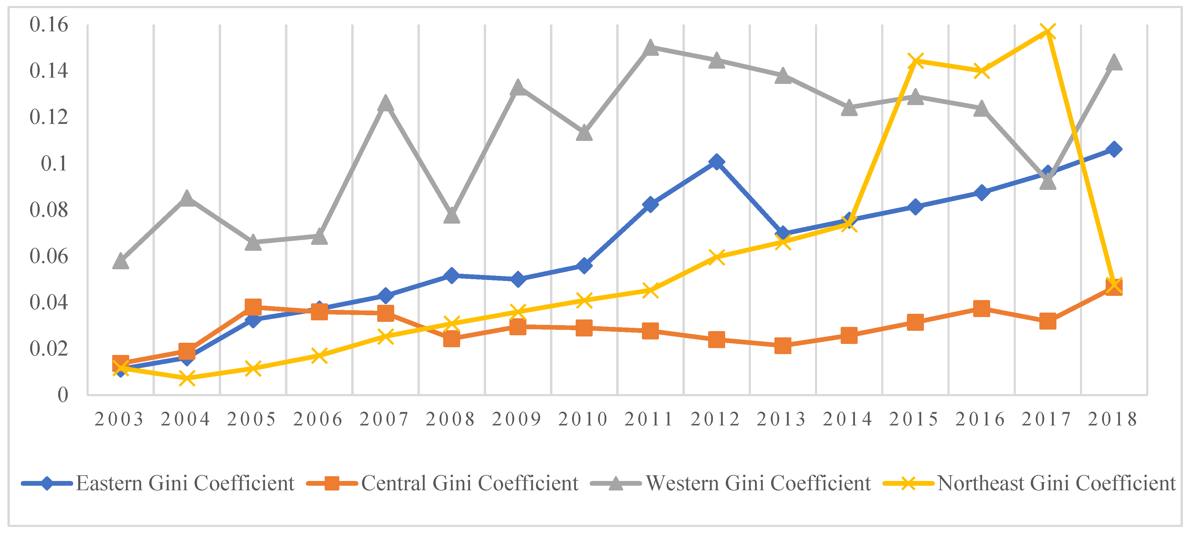
Figure 3 and Table 3 show that, overall, the four regions’ intra-regional differences in industrial GTFP have gradually widened. More specifically, (1) the eastern region has the fastest expansion rate of Gini coefficient with an average annual expansion rate of 56.46%, followed by northeast China with an annual growth rate of 20.60%, the central region with 16.0%, and the western region with 9.86%. (2) The eastern region showed an N-shape trend of “upward-downward-upward” during the sample period, showing an overall trend of widening intra-regional differences; the Gini coefficient in the central region was relatively stable, increasing gradually from 0.014 to 0.046. The Gini coefficient in western China shows frequent “enlarging and narrowing” fluctuations, indicating that the GTFP of different provinces in western China keeps changing with poor stability. As for the northeast region, its Gini coefficient of GTFP showed steady growth from 2003 (0.0116) to 2014 (0.0738), with an average annual growth rate of 48.62%. However, from 2014 to 2015, its Gini coefficient increased sharply from 0.0738 to 0.1444, with a growth rate of 95.69%. This may be due to the drastic increase of Jilin Province’s industrial GTFP from 2014 to 2015, because its industrial value added remained stable while the energy input was reduced by nearly 20%. Subsequently, from 2017 to 2018, northeast China’s Gini coefficient declined precipitously from 0.157 in 2017 to 0.0475 in 2018. (3) Overall, western China has the highest intra-regional difference in GTFP growth, followed by the eastern, northeast, and central regions.

5.2.3. Inter-Regional Differences

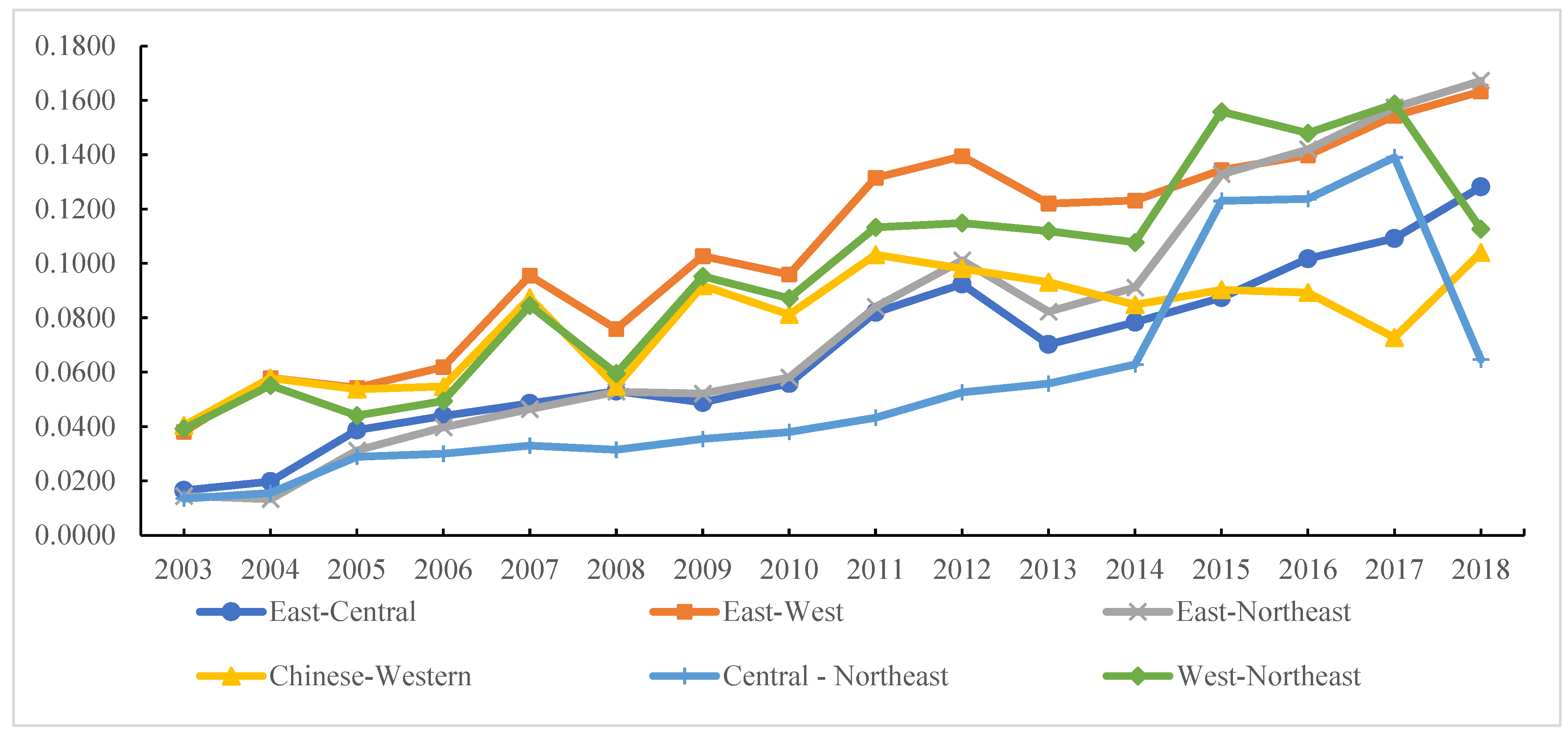
Figure 4 and Table 4 show that the regional differences of industrial GTFP exhibit significant fluctuations and an overall upward trend. In terms of the size of inter-regional Gini coefficients, the east-west region has the largest inter-regional difference, followed by the west-northeast region, east-northeast region, and central-west region. The central-northeast region has the smallest inter-regional difference, whereas the east-northeast differences show the greatest fluctuations. In terms of the trend of inter-regional differences in Gini coefficients, all the pairwise GTFP Gini coefficients exhibit an upward trend. More specifically, (1) the Gini coefficient of GTFP in eastern China vs. central, western, and northeast China expanded from 0.0165, 0.038, and 0.0145 in 2003 to 0.128, 0.163, and 0.167 in 2018, with an average annual growth rate of 45.034%, 21.932%, and 70.416%, respectively. The Gini coefficient of central vs. western China and northeast China expanded from 0.0404 and 0.0134 in 2003 to 0.104 and 0.0646 in 2018, with annual growth rates of 10.513% and 25.337%. Finally, the annual growth rate of the inter-regional Gini coefficient of western vs. northeast China was 12.526%. Thus, the variation of inter-regional differences is the largest for the east-northeast region, followed by the east-central region, central-northeast region, east-west region, and west-northeast region, and the central-west region has the smallest variation. (2) From 2003 to 2011, the fluctuation patterns of east-west, central-west, and west-northeast regional differences were highly similar, and all experienced an “up-down” movement in the adjacent years. These three inter-regional fluctuations became dissimilar from 2011 to 2018. For example, the Gini coefficient in the central-west region decreased in most years, showing a decreasing trend in the difference. Meanwhile, the Gini coefficient in the eastern-western regions increased year by year, showing the widening of regional difference. The western-northeast regional differences fluctuated wildly, presenting an “M” shape, showing a general downward trend.

5.2.4. Sources of Differences

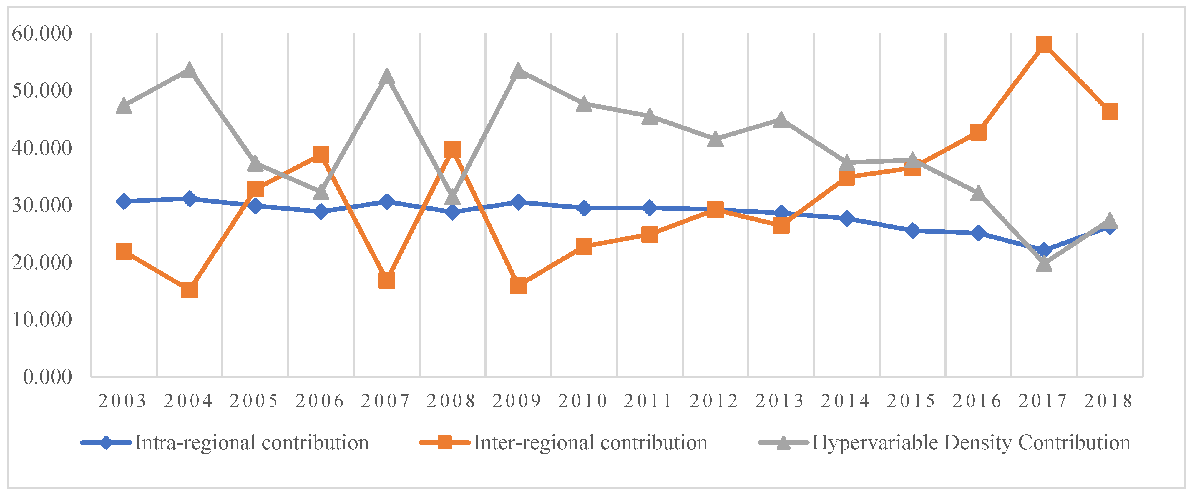
Table 5 and Figure 5 describe the source contribution rate and its variation trend of China’s industrial GTFP. The contribution rate of intra-regional differences decreased slightly from 30.685% in 2003 to 26.285% in 2018, with an average annual declining rate of 0.956%. The contribution rate ranged from 22.118% to 31.150%, with an average contribution rate of 28.383%. This indicates that the intra-regional differences are not the main source of regional differences, and the degree of influence shows a decreasing trend. The contribution of inter-regional differences includes the contribution of an inter-regional net difference and regional super variable density. As shown in Figure 5, inter-regional differences are the primary source of uneven distribution of industrial GTFP, with an average contribution rate of 71.617%. Among the inter-regional differences, the contribution of the inter-regional super variable net value difference shows an increasing trend, with extensive fluctuations rising from 21.896% in 2003 to 46.314% in 2018. The contribution rate ranged from 15.18% to 58.05%, with an annual growth rate of 7.435%, and an average contribution rate of 31.439%. The contribution of inter-regional super variable density decreased from 47.418% in 2003 to 27.4% in 2018, with an average annual decline rate of 2.814%, indicating a decreasing trend of the inter-regional differences caused by overlapping problems between different regions. However, the net difference of total factor productivity between different regions is larger and increasing, leading to the uneven distribution of GTFP across regions and over time.

5.3. Spatial-Temporal Heterogeneity Analysis of Influencing Factors of GTFP in Chinese Industry

The above analysis of the regional gap of GTFP in China’s industry reveals that natural endowment, economic, geographical, and intellectual and institutional factors exert different impacts on the enterprise production and productivity. It also suggests that the key to narrowing the regional gap is to incorporate these different influencing factors into forming effective regional industrial development policies.
In addition, as the industrial structure is constantly evolving in different stages, the effects of relevant influencing factors will also change in different periods. Thus, we need to explore the spatial-temporal heterogeneity of the effects on GTFP from such influencing factors as factor supply, technological progress, structural factors, and market environment. The OLS model, time-weighted regression (TWR), geo-weighted regression (GWR), and spatial-temporal geographically weighted regression (GTWR) were used for regression analysis. The application of the GTWR model is more sensitive to multicollinearity among variables. Therefore, we conducted variance inflation factor tests (VIF) on the variables. The results are shown in Table 6. The VIFs are all less than 10, indicating that the estimation is free from the multicollinearity problem among the variables.
Before using the GTWR model, we proceeded to test the spatial-temporal non-stationarity of the data. A common approach is to compare the quartiles of GTWR (i.e., the difference between the lower and upper quartiles) with twice the standard error of the OLS model. If there is a significant difference, it indicates the presence of spatial-temporal non-stationarity [34,45]. Table 7 shows that there is a significant difference between the interquartile value and two times the OLS standard error, i.e., there is spatial-temporal non-stationarity in the variables influencing GTFP. Therefore, it is appropriate for us to employ the GTWR model to consider the spatial-temporal complexity of the influencing factors on GTFP.
To provide more empirical evidence, we show the coefficient regression results of different models in the paper. Following Yuan [46], we compare the coefficients of the TWR model, GWR model, and GTWR model regression results (see Table 8).
Table 9 compares the regression attributes and results of the globe-OLS, TWR, GWR, and GTWR models. It appears that the GTWR model performs the best, having a higher goodness of fit and a lower AIC, indicating that it is reasonable to use the GTWR model to investigate the spatial-temporal heterogeneities of China’s industrial GTFP.
Figure 6 shows the spatial-temporal heterogeneity of the impact of factor inputs on GTFP. The impact of capital input on GTFP is ineffective, consistent with the previous analysis of a low level of technical efficiency. The more advanced a region’s economic level, the stronger the crowding-out effect of capital input on green industrial development, and it is only in northeast China that the capital input has a promoting effect on GTFP. In terms of energy structure, traditional energy does not strongly constrain GTFP in the eastern and central regions. This is due to the rapid energy structure transformation in those regions, where the early application of natural gas and other clean energy and related technologies has gradually reduced dependence on traditional energy in the regions. Northeast China is dominated by heavy industry and resource-based industry and has a well-established industrial base, so the traditional energy structure has a strong positive effect on GTFP. In contrast, western China has a weak industrial base and a strong “resource curse.” Therefore, in the formulation of regional capacity elimination-related policies, it is necessary to consider local conditions when carrying out production suspension and enterprise transformation so as to avoid abrupt enterprise closure, causing a massive negative impact on local economic growth.
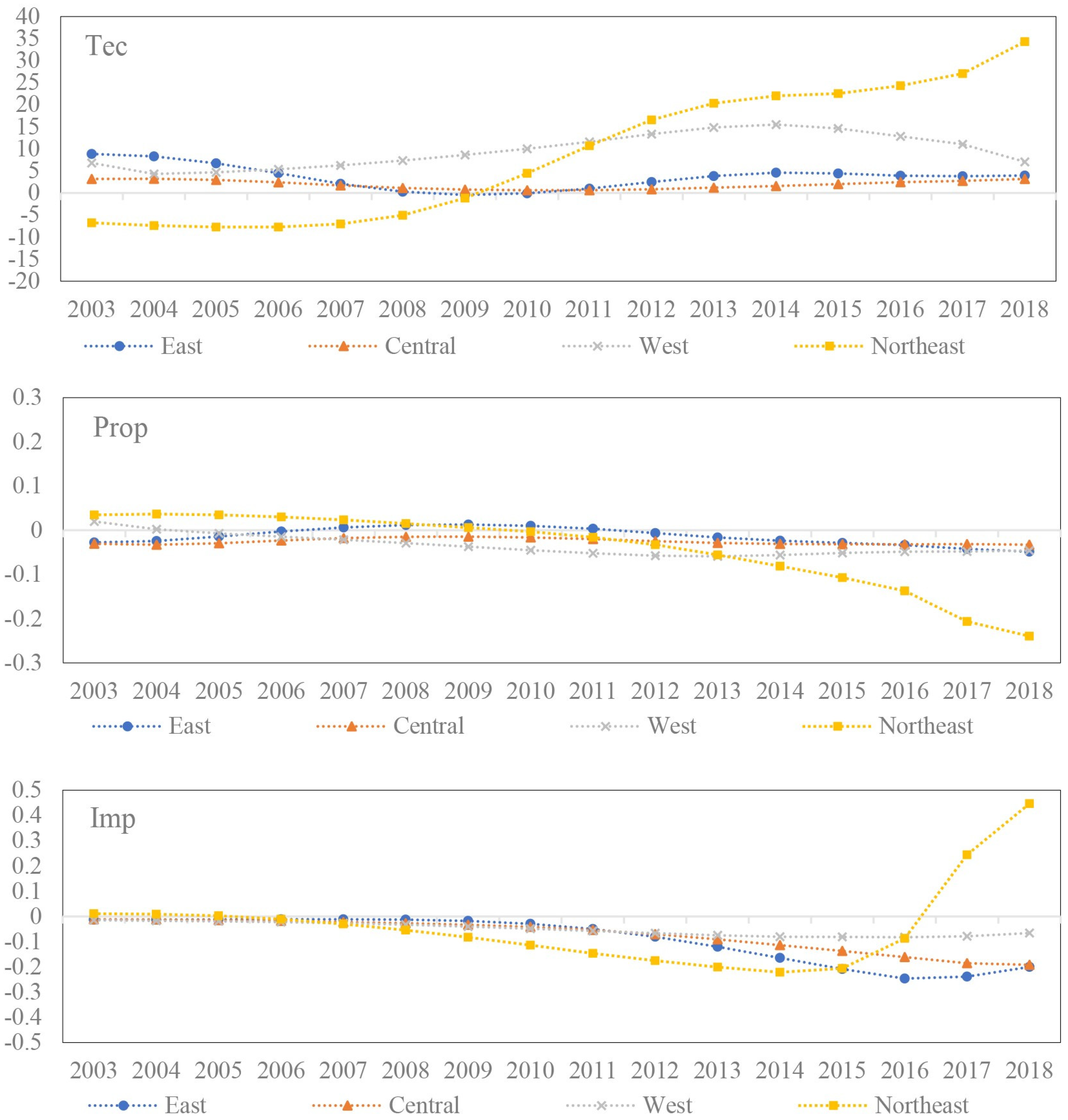
Figure 7 shows the spatial-temporal heterogeneity of the impact of technological progress on GTFP. Science and technology input (R&D investment) appears to be an important factor promoting industrial GTFP, with such positive impact increasing gradually after 2009 and a more prominent impact in the northeast and western regions. Overall, the number of industrial enterprises’ patent applications (Prop) appears to have a “crowding out effect” on GTFP. It is only in Shanghai, Zhejiang, Fujian, and Jiangxi Provinces that the number of industrial enterprises’ patent applications has an increasing promoting effect on GTFP. This may be due to a prolonged lag from patent applications to commercialization and industrial application. While China’s patent application number has grown by leaps and bounds in recent years, the applicable patent technology conversion rate and diffusion efficiency are still low, resulting in the mismatch between patent growth and productivity growth. The import and introduction of technology is gradually showing a “crowding out effect” on GTFP. In the eastern and central provinces, the higher the dependence of local industrial enterprises on external technology import and absorption, the stronger the crowding-out effect on GTFP. China has entered a critical period from technology introduction, imitation, and transformation to independent innovation. Independent research and development capacity is linked to sustainable economic growth. Therefore, it is imperative to continue to increase scientific and technological input in various regions to promote the sustainable growth of GTFP. Meanwhile, it is important to incentivize and reward practical patent developments and clean technology projects so as to accelerate the transformation of intellectual property rights toward fundamental and practical productions.
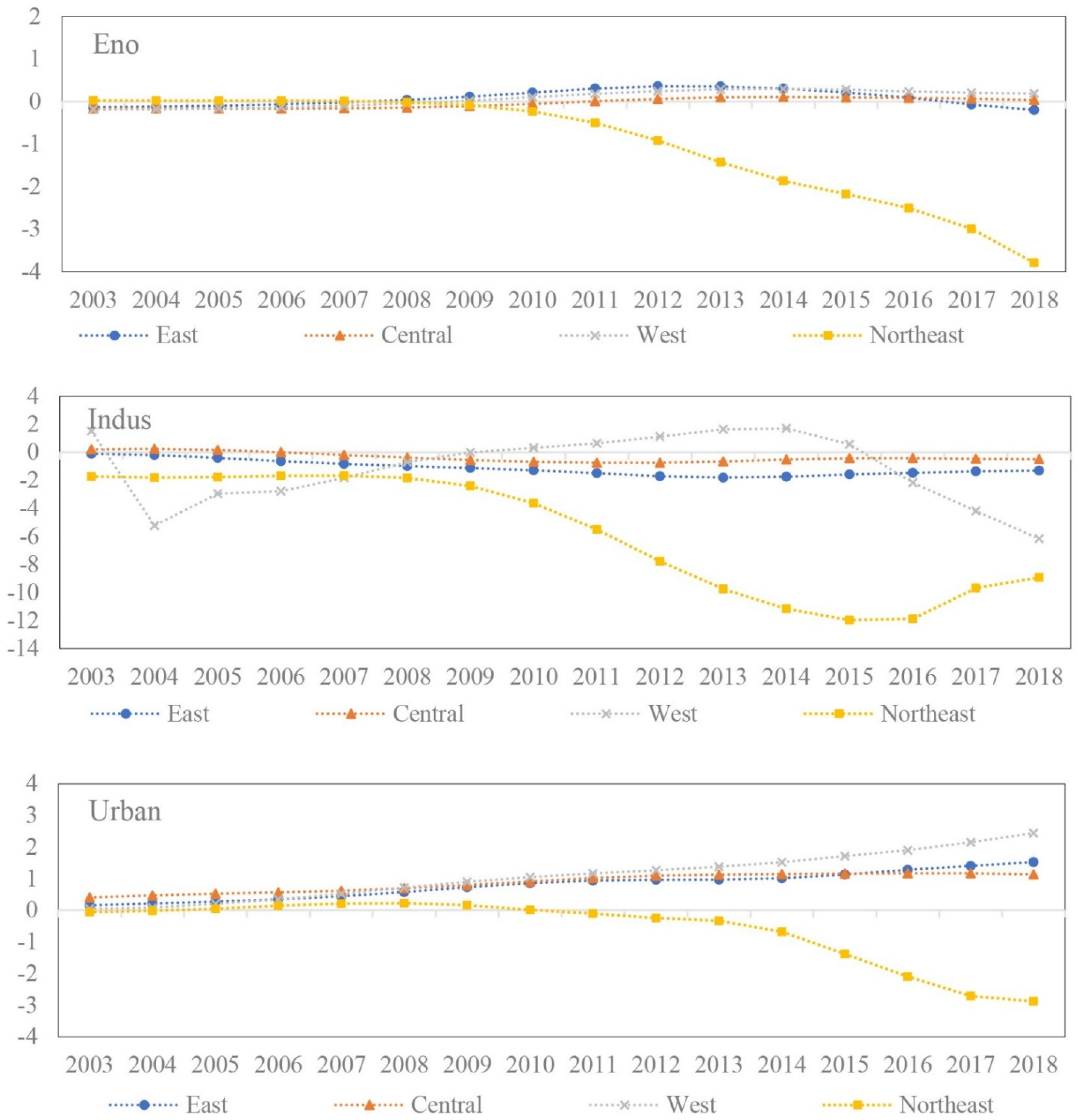
Figure 8 shows the spatial-temporal heterogeneity of the impact of structural factors on GTFP. The level of industrial pollution control (Eno) has a heterogeneous effect on GTFP across regions, and the marginal promoting effect gradually decreased and exhibited an “inverted U-shape” pattern of first increase and then decline for the eastern, central, and western regions. For the northeast region, environmental governance showed an increasingly negative effect on GTFP. This may be caused by the high marginal cost of industrial pollution control, and the reduction of high-pollution and high-emission industries has a tremendous negative impact on the industrial capacity in northeast China. Altogether, this suggests that more robust environmental regulation policies have a limited and diminishing effect on promoting the growth of GTFP.
The agglomeration level of industrial enterprises (Indus) inhibits GTFP growth in the eastern and central regions and has a strong “crowding out effect” in the northeast region. Only in the western region did industrial agglomeration have an effective practical scale effect to significantly promoting GTFP growth during the 11th and 12th “Five-Year Plan” periods when this region benefited from the transfer of many industries from the eastern region. However, the dividend from such industrial transfer began to decline after 2015 for the western region. Thus, industrial clustering has not brought forth the expected sustainable GTFP growth to the central and western regions.
Urbanization level (urban) appears to have a diverse effect on GTFP, showing a promotion effect in the eastern, central, and western regions, but a crowding-out effect in the northeast region, and the regional gap has further widened since 2010. It reflects the need to pay more attention to the problem of labor loss in the northeast’s urbanization process, and if the need is not addressed, the gap in industrial efficiency between regions will continue to widen and further worsen the “Decline of Northeast China”.
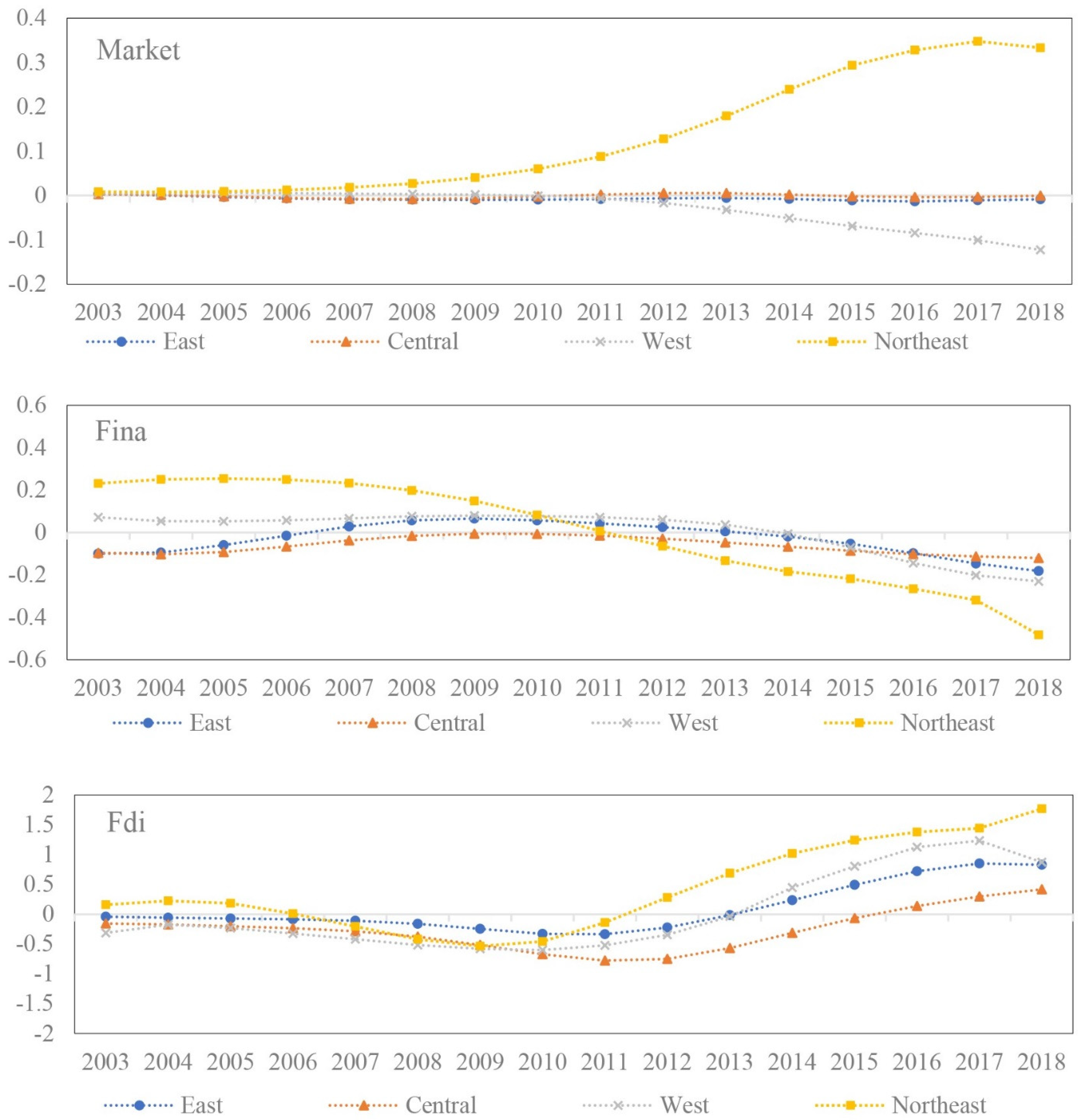
Figure 9 shows the spatial-temporal heterogeneity of the impact of the market environment on GTFP. The degree of marketization (market) has little effect on industrial enterprises’ GTFP in the eastern and central regions, indicating that marketization is not the main factor for improving GTFP growth of industrial enterprises in those regions. However, the degree of marketization strongly affects the less developed northeast and western regions with a positive effect on the northeast and a negative effect on the western region. Driven by the plan to “revitalize northeast China”, this region has fully absorbed the policy dividend brought by the reform of state-owned enterprises in the process of marketization, and its production efficiency has significantly improved.
The level of financial deepening (fina) has an “inverted U-shaped” effect on the GTFP of Chinese industry as a whole. The influence of financial support on GTFP weakened in all regions in 2010 and turned from positive to negative after 2014. With technological progress and continuous economic growth, financial resources flowed from the industrial sector to the service sector, which led to the decline in the growth rate of industrial output value and employment share, thus inhibiting the growth of industrial GTFP. Foreign direct investment (FDI) has a U-shaped dynamic impact on industrial GTFP. Out of all regions, FDI has the lowest marginal effect on GTFP in central China. Compared with other regions that are increasingly attracting high-quality foreign investment, especially in the high-tech sector, and the gradual release of dividends from opening up, the central region has a large scale of industrial enterprises but a relatively small scale of FDI, coupled with a not reasonable enough investment structure, leading to the inefficient use of foreign capital in this region. In the future, China’s regions should actively adjust the structure of FDI and pay attention to the quality and scale of FDI introduction.

6. Conclusions and Policy Recommendations

6.1. Summary and Conclusions

The major findings of this study are as follows:
(1)
From 2003 to 2018, China’s industrial GTFP exhibited an overall dynamic trend of “growth-steady growth-decline”. The growth rate of eastern China was much higher than that of other regions, and the GTFP of northeast and western China fluctuated widely after 2016. The decomposition analysis reveals that the technical efficiency of China’s industrial sector has lowered the GTFP, and technological progress is an essential source of promoting the growth of China’s industrial GTFP.
(2)
The western region has the greatest intra-regional differences in GTFP growth, followed by the eastern and northeast regions, and the central region has the smallest intra-regional differences. The primary source of the uneven distribution of GTFP in industry is inter-regional difference, with the average contribution rate to Gini coefficient at 71.617%. The regional difference in GTFP is gradually widening.
(3)
From the perspective of factor supply, technological innovation, government regulation, and external environment, there is significant spatial and temporal heterogeneity in the impact of different factors on industrial GTFP in China’s four regions. For the eastern, central, and western regions, (i) the input of science and technology and the level of urbanization have a long-term promoting effect on GTFP. (ii) The influence of FDI on GTFP has experienced an “N-type” fluctuation of first promoting, then inhibiting, and then promoting. (iii) Capital input, patent output, and technology import have a long-term negative impact on GTFP. (iv) Environmental governance and financial support have a “U-shaped” impact on the eastern, central, and western regions. In northeast China, (i) capital drive, energy structure, and marketization process exert a positive impact, (ii) while environmental governance and urbanization have a strong negative impact. (iii) Scientific and technological input has a U-shaped influence on GTFP, and (iv) financial support has the inverse U-shape effect.

6.2. Policy Recommendations

At present, the gap in GTFP in China’s industry is expanding. Therefore, differentiated regional policies that consider regional differences in the development status should be carried out to prevent further expansion of regional industrial imbalance. To promote the coordinated development of China’s industrial sectors, policy makers should formulate differentiated industrial policies according to the heterogeneous effects of different factors on GTFP found in this study. More specifically:
(1)
Promote coordinated development across regions and form an industrial layout connecting regions with complementary advantages and reasonable division of labor. Initiate a new round of urbanization to accelerate industrial transfer, to promote employment and infrastructure construction (such as transportation, logistics, medical services, and environmental protection), and to optimize urban spatial planning and promote the cross-regional flow of factors of production. In particular, more attention should be paid to mitigating the impact of population loss in northeast China.
(2)
Accelerate industrial transformation and structural upgrading, and through technological innovation, drive high-quality industrial development. In addition, increase the share of advanced manufacturing in industry and strengthen financial support for the real economy to ease the difficulty faced by industrial enterprises in obtaining loans. Meanwhile, promote sustained innovation by enterprises and encourage high-quality industrial development through boosting investment in scientific and technological innovation and taking measures to accelerate the application of scientific and technological achievements.
(3)
Diversify environmental regulation policies (again, considering regional heterogeneities) and vigorously promote cleaner production. As the marginal effect of environmental governance energy efficiency decreases in the eastern and central regions, the development mode needs to be changed by starting from the technology source and adopting the “three-pronged” management mode of energy saving, carbon reduction, and pollution control.
(4)
Promote industrial clustering and improve the efficiency of intensive land use. Industrial agglomeration without scale efficiency is a common problem in all major regions of China. The first step to address the problem of low FDI utilization efficiency in the central region is to establish an effective exchange platform so as to expedite local absorption of FDI advanced production technology. Second, promote effective agglomeration of upstream and downstream enterprises of the industrial chain, reduce logistics costs, further improve industrial production efficiency, and fully transform technological advantages into economic advantages.

Author Contributions

Original draft preparation, S.X.; Data curation and Methodology, S.W.; Review, revision, and editing, F.Z.; Formal analysis, W.-C.H. All authors have read and agreed to the published version of the manuscript.

Funding

This research received funding support from “the Key Project of Philosophy and Social Science Research in Colleges and Universities in Hubei Province” (21ZD155) and “the Key Project of Social Sciences in Guizhou Province” (20GZZB22).

Institutional Review Board Statement

Not applicable.

Informed Consent Statement

Not applicable.

Data Availability Statement

Data are available from the authors upon reasonable request, as the data need further use.

Acknowledgments

We are grateful for the insightful comments and suggestions made by the editor and anonymous reviewers.

Conflicts of Interest

The authors declare no conflict of interest.

References

  1. Rahman, M.M.; Kashem, M.A. Carbon emissions, energy consumption and industrial growth in Bangladesh: Empirical evidence from ARDL cointegration and Granger causality analysis. Energy Policy 2017, 110, 600–608. [Google Scholar] [CrossRef]
  2. Shahbaz, M.; Lean, H.H.; Shabbir, M.S. Environmental Kuznets Curve hypothesis in Pakistan: Cointegration and Granger causality. Renew. Sustain. Energy Rev. 2012, 16, 2947–2953. [Google Scholar] [CrossRef] [Green Version]
  3. Waheed, R.; Sarwar, S.; Wei, C. The survey of economic growth, energy consumption and carbon emission. Energy Rep. 2019, 5, 1103–1115. [Google Scholar] [CrossRef]
  4. Jiang, T.; Huang, S.; Yang, J. Structural carbon emissions from industry and energy systems in China: An input-output analysis. J. Clean. Prod. 2019, 240, 118116. [Google Scholar] [CrossRef]
  5. Li, K.; Lin, B. Impact of energy conservation policies on the green productivity in China’s manufacturing sector: Evidence from a three-stage DEA model. Appl. Energy 2016, 168, 351–363. [Google Scholar] [CrossRef]
  6. Yang, Z.; Fan, M.; Shao, S.; Yang, L. Does carbon intensity constraint policy improve industrial green production performance in China? A quasi-DID analysis. Energy Econ. 2017, 68, 271–282. [Google Scholar] [CrossRef]
  7. Cheng, M.; Shao, Z.; Gao, F.; Yang, C.; Tong, C.; Yang, J.; Zhang, W. The effect of research and development on the energy conservation potential of China’s manufacturing industry: The case of east region. J. Clean. Prod. 2020, 258, 120558. [Google Scholar] [CrossRef]
  8. Wang, Q.; Zhao, C. Regional difference and driving factors of industrial carbon emissions performance in China. Alex. Eng. J. 2021, 60, 301–309. [Google Scholar] [CrossRef]
  9. Fu, S.; Ma, Z.; Ni, B.; Peng, J.; Zhang, L.; Fu, Q. Research on the spatial differences of pollution-intensive industry transfer under the environmental regulation in China. Ecol. Indic. 2021, 129, 107921. [Google Scholar] [CrossRef]
  10. Yalçınkaya, Ö.; Hüseyni, İ.; Çelik, A.K. The Impact of Total Factor Productivity on Economic Growth for Developed and Emerging Countries: A Second-generation Panel Data Analysis. Margin J. Appl. Econ. Res. 2017, 11, 404–417. [Google Scholar] [CrossRef]
  11. Chen, S.Y. Green industrial revolution in China: A perspective from the change of environmental total factor productivity. Econ. Res. J. 2010, 45, 21–34. [Google Scholar]
  12. Chen, S.; Golley, J. ‘Green’ productivity growth in China’s industrial economy. Energy Econ. 2014, 44, 89–98. [Google Scholar] [CrossRef]
  13. Zhang, J.; Tan, W. Study on the green total factor productivity in main cities of China. Zb. Rad. Ekon. Fak. Rijeci Časopis Ekon. Teor. Praksu 2016, 34, 215–234. [Google Scholar]
  14. Wang, K.; Wei, Y.-M. Sources of energy productivity change in China during 1997–2012: A decomposition analysis based on the Luenberger productivity indicator. Energy Econ. 2016, 54, 50–59. [Google Scholar] [CrossRef]
  15. Xia, F.; Xu, J. Green total factor productivity: A re-examination of quality of growth for provinces in China. China Econ. Rev. 2020, 62, 101454. [Google Scholar] [CrossRef]
  16. Yin, J.-Y.; Cao, Y.-F.; Tang, B.-J. Fairness of China’s provincial energy environment efficiency evaluation: Empirical analysis using a three-stage data envelopment analysis model. Nat. Hazards 2019, 95, 343–362. [Google Scholar] [CrossRef]
  17. Wang, C. Decomposing energy productivity change: A distance function approach. Energy 2007, 32, 1326–1333. [Google Scholar] [CrossRef]
  18. Wang, Z.; Feng, C. Sources of production inefficiency and productivity growth in China: A global data envelopment analysis. Energy Econ. 2015, 49, 380–389. [Google Scholar] [CrossRef]
  19. Yang, L.; Ouyang, H.; Fang, K.; Ye, L.; Zhang, J. Evaluation of regional environmental efficiencies in China based on super-efficiency-DEA. Ecol. Indic. 2015, 51, 13–19. [Google Scholar]
  20. Wang, F.; Li, R.; Yu, C.; Xiong, L.; Chang, Y. Temporal-Spatial Evolution and Driving Factors of the Green Total Factor Productivity of China’s Central Plains Urban Agglomeration. Front. Environ. Sci. 2021, 9, 193. [Google Scholar] [CrossRef]
  21. Chung, Y.H.; Färe, R.; Grosskopf, S. Productivity and Undesirable Outputs: A Directional Distance Function Approach. J. Environ. Manag. 1997, 51, 229–240. [Google Scholar] [CrossRef] [Green Version]
  22. Oh, D.-H.; Heshmati, A. A sequential Malmquist–Luenberger productivity index: Environmentally sensitive productivity growth considering the progressive nature of technology. Energy Econ. 2010, 32, 1345–1355. [Google Scholar]
  23. Oh, D.-h. A global Malmquist-Luenberger productivity index. J. Product. Anal. 2010, 34, 183–197. [Google Scholar] [CrossRef]
  24. Liu, G.; Wang, B.; Zhang, N. A coin has two sides: Which one is driving China’s green TFP growth? Econ. Syst. 2016, 40, 481–498. [Google Scholar]
  25. Hu, J.-L.; Sheu, H.-J.; Lo, S.-F. Under the shadow of Asian Brown Clouds: Unbalanced regional productivities in China and environmental concerns. Int. J. Sustain. Dev. World Ecol. 2009, 12, 429–442. [Google Scholar] [CrossRef]
  26. Dan, S. Regional Differences in China’s Energy Efficiency and Conservation Potentials. China World Econ. 2007, 15, 96–115. [Google Scholar]
  27. Du, J.L.; Liu, Y.; Diao, W.X. Assessing Regional Differences in Green Innovation Efficiency of Industrial Enterprises in China. Int. J. Environ. Res. Public Health 2019, 16, 940. [Google Scholar]
  28. Chen, Y.; Yin, G.; Liu, K. Regional differences in the industrial water use efficiency of China: The spatial spillover effect and relevant factors. Resour. Conserv. Recycl. 2021, 167, 105239. [Google Scholar]
  29. Wang, D.T.; Gu, F.F.; Tse, D.K.; Yim, C.K. When does FDI matter? The roles of local institutions and ethnic origins of FDI. Int. Bus. Rev. 2013, 22, 450–465. [Google Scholar]
  30. Xu, B.; Lin, B.Q. Regional differences in the CO2 emissions of China’s iron and steel industry: Regional heterogeneity. Energy Policy 2016, 88, 422–434. [Google Scholar]
  31. Yan, Z.; Zou, B.; Du, K.; Li, K. Do renewable energy technology innovations promote China’s green productivity growth? Fresh evidence from partially linear functional-coefficient models. Energy Econ. 2020, 90, 104842. [Google Scholar] [CrossRef]
  32. Gao, Y.; Zhang, M.; Zheng, J. Accounting and determinants analysis of China’s provincial total factor productivity considering carbon emissions. China Econ. Rev. 2021, 65, 101576. [Google Scholar] [CrossRef]
  33. Wei, W.; Zhang, W.-L.; Wen, J.; Wang, J.-S. TFP growth in Chinese cities: The role of factor-intensity and industrial agglomeration. Econ. Model. 2020, 91, 534–549. [Google Scholar] [CrossRef]
  34. Fotheringham, A.S.; Crespo, R.; Yao, J. Geographical and Temporal Weighted Regression (GTWR). Geogr. Anal. 2015, 47, 431–452. [Google Scholar] [CrossRef] [Green Version]
  35. Tao, F.; Zhang, H.; Hu, J.; Xia, X.H. Dynamics of green productivity growth for major Chinese urban agglomerations. Appl. Energy 2017, 196, 170–179. [Google Scholar] [CrossRef]
  36. Fare, R.; Grosskopf, S.; Pasurkajr, C. Environmental production functions and environmental directional distance functions. Energy 2007, 32, 1055–1066. [Google Scholar] [CrossRef]
  37. Lin, B.; Chen, Z. Does factor market distortion inhibit the green total factor productivity in China? J. Clean. Prod. 2018, 197, 25–33. [Google Scholar] [CrossRef]
  38. Dagum, C. A new approach to the decomposition of the Gini income inequality ratio. Empir. Econ. 1997, 22, 515–531. [Google Scholar] [CrossRef]
  39. Huang, B.; Zhang, L.; Wu, B. Spatiotemporal analysis of rural-urban land conversion. Int. J. Geogr. Inf. Sci. 2009, 23, 379–398. [Google Scholar] [CrossRef]
  40. Shao, S.; Yang, L.; Yu, M.; Yu, M. Estimation, characteristics, and determinants of energy-related industrial CO2 emissions in Shanghai (China), 1994–2009. Energy Policy 2011, 39, 6476–6494. [Google Scholar] [CrossRef]
  41. Fan, M.; Shao, S.; Yang, L. Combining global Malmquist–Luenberger index and generalized method of moments to investigate industrial total factor CO2 emission performance: A case of Shanghai (China). Energy Policy 2015, 79, 189–201. [Google Scholar] [CrossRef]
  42. Wang, K.L.; Pang, S.Q.; Ding, L.L.; Miao, Z. Combining the biennial Malmquist-Luenberger index and panel quantile regression to analyze the green total factor productivity of the industrial sector in China. Sci. Total Environ. 2020, 739, 140280. [Google Scholar] [CrossRef]
  43. Ren, Y. Research on the green total factor productivity and its influencing factors based on system GMM model. J. Ambient. Intell. Humaniz. Comput. 2019, 11, 3497–3508. [Google Scholar] [CrossRef]
  44. Wang, K.; Wei, Y.-M. China’s regional industrial energy efficiency and carbon emissions abatement costs. Appl. Energy 2014, 130, 617–631. [Google Scholar] [CrossRef]
  45. Ma, X.; Zhang, J.; Ding, C.; Wang, Y. A geographically and temporally weighted regression model to explore the spatiotemporal influence of built environment on transit ridership. Comput. Environ. Urban Syst. 2018, 70, 113–124. [Google Scholar] [CrossRef]
  46. Yuan, H.; Feng, Y.; Lee, J.; Liu, H. The Spatio-Temporal Heterogeneity of Financial Agglomeration on Green Development in China Cities Using GTWR Model. Sustainability 2020, 12, 6660. [Google Scholar] [CrossRef]
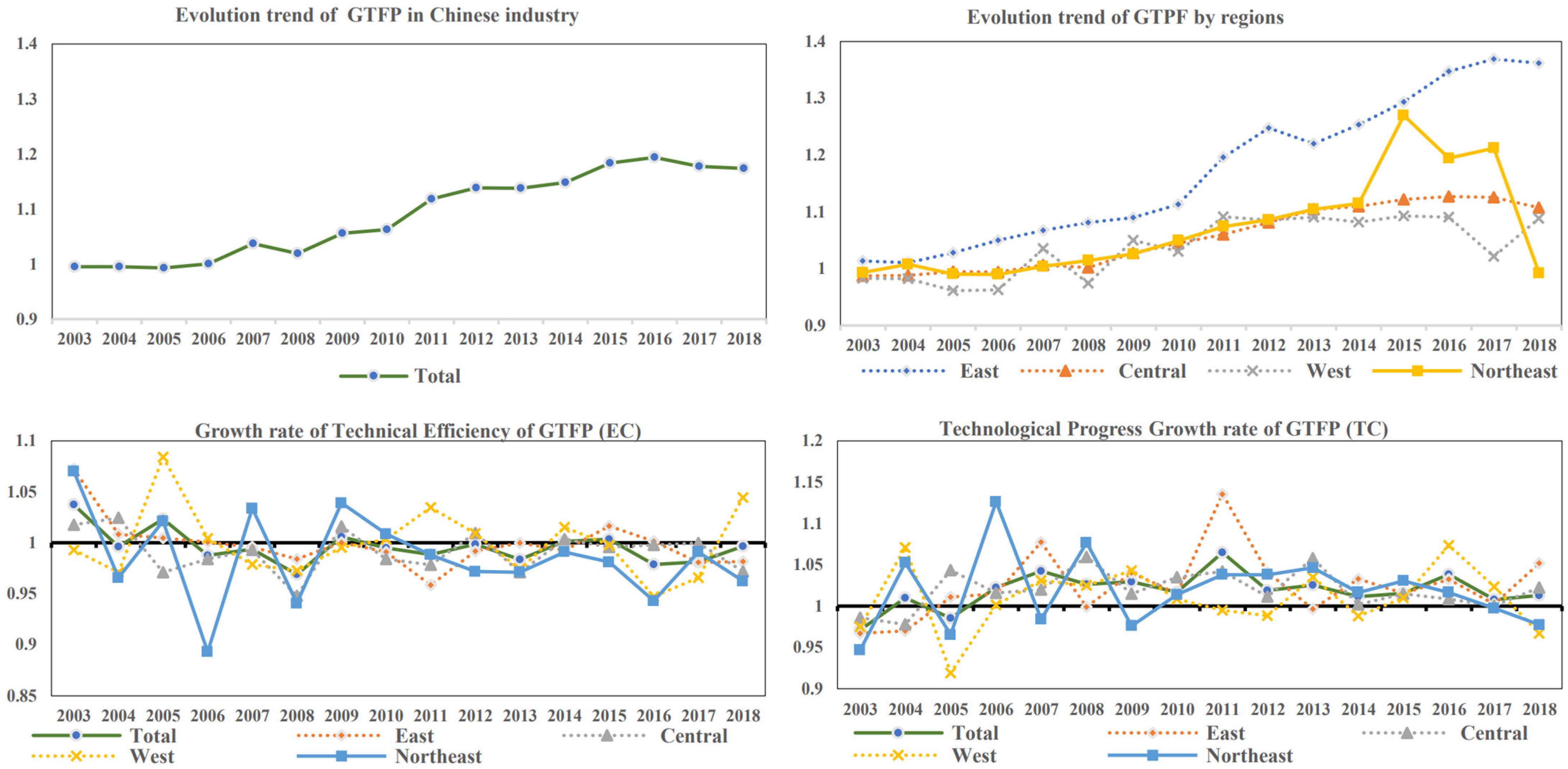
Figure 1. Changing trend and decomposition of growth rate of GTFP in China’s industry from 2003 to 2018.
Sustainability 14 09229 g001
Figure 2. Overall Gini coefficient of GTFP in China’s industry from 2003 to 2018.
Sustainability 14 09229 g002
Figure 3. Intra-regional Gini coefficient of China’s industrial GTFP from 2003 to 2018.
Sustainability 14 09229 g003
Figure 4. Inter-regional (pairwise) differences in Gini coefficient of industrial GTFP from 2003 to 2018.
Sustainability 14 09229 g004
Figure 5. Source contribution rates of industrial GTFP.
Sustainability 14 09229 g005
Figure 6. Spatial-temporal heterogeneity analysis of the impact of input factors on GTFP.
Sustainability 14 09229 g006
Figure 7. Spatial-temporal heterogeneity analysis of the impact of technological progress on GTFP.
Sustainability 14 09229 g007
Figure 8. Spatial-temporal heterogeneity of structural factors on GTFP.
Sustainability 14 09229 g008
Figure 9. Spatial-temporal heterogeneity analysis of the impact of market environment on GTFP.
Sustainability 14 09229 g009
Table 1. The variables used in econometric analysis of GTFP influencing factors.
First Level IndicatorsSecond Level IndicatorsVariableMeasuring Method
Factor supplyCapital inputFxRatio of new fixed capital input of industrial enterprises to GDP
Energy structureEnergyRatio of coal consumption to energy consumption
Technological progressR&D investmentTecRatio of R&D internal expenditure to GDP
Patent applicationsPropLogarithm of patent applications of industrial enterprises above designated size with one year lag
Technical modificationImpRatio of total expenditure of industrial enterprises above designated size in technology introduction, adaptation, and absorption to GDP
Structural factorsEnvironmental governanceEnoRatio of investment in local industrial pollution control to GDP
Industrial clusteringIndusLocation quotient
Urbanization levelUrbanUrbanization rate
Market environmentDegree of marketizationMarketMarketization index
Financial developmentFinaRatio of outstanding loans of financial institutions to GDP
Foreign direct investmentFDIRatio of total foreign investment to GDP
Table 2. Descriptive statistics.
VarNameObsMeanSDMinMedianMax
Capital stock5107369.45886478.345290.095676.4635,890.02
Labor input510278.7029304.83810.42169.041568.00
Energy consumption5107029.65665035.299186.926104.0126,726.53
Expected output5104890.93675509.60683.783102.0534,421.81
So251065.622344.1291.0655.64200.30
Co2510258.3891185.18814.00205.80912.20
Gtfp4801.08940.20980.56071.04401.8312
Fx4800.50490.18450.22530.46571.3264
Energy4800.95670.39060.03800.89592.4229
Tec4800.01390.01060.00170.01090.0617
Prop4807.31301.97071.94597.301912.5750
Imp4800.99250.84600.06640.71675.7127
Eno4800.00160.00130.00010.00130.0099
Indus4800.01340.02350.00000.00430.1322
Urban4800.52380.14410.25660.50500.8960
Market4806.46131.89962.33006.270011.7100
Fina4801.19430.41560.53721.11832.5847
FDI4800.05830.06950.00660.03070.7503
Table 3. Overall and intra-regional Gini coefficient of industrial GTFP.
YearTotalEastCentralWestNortheast
20030.03140.01120.01370.05800.0116
20040.04470.01600.01890.08510.0073
20050.04670.03250.03790.06590.0114
20060.05120.03710.03580.06860.0170
20070.07670.04280.03530.12630.0253
20080.06010.05150.02430.07770.0308
20090.08190.04990.02950.13300.0359
20100.07730.05580.02890.11340.0409
20110.10480.08230.02760.15020.0452
20120.11040.10070.02380.14460.0595
20130.09620.06960.02130.13800.0660
20140.09610.07550.02570.12420.0738
20150.11200.08130.03140.12890.1444
20160.11540.08740.03730.12390.1400
20170.11750.09580.03180.09240.1572
20180.12850.10610.04640.14380.0475
Table 4. Inter-regional (pairwise) difference in Gini coefficient of industrial GTFP.
YearEast-CentralEast-WestEast-NortheastCentral-WestCentral-NortheastWest-Northeast
20030.01650.03800.01450.04040.01350.0391
20040.01980.05790.01330.05790.01550.0551
20050.03870.05430.03120.05370.02890.0440
20060.04390.06180.03970.05470.03000.0494
20070.04850.09550.04640.08730.03300.0845
20080.05300.07590.05280.05480.03140.0595
20090.04880.10270.05210.09190.03540.0952
20100.05580.09590.05800.08120.03800.0872
20110.08200.13150.08400.10320.04330.1133
20120.09240.13940.10110.09810.05260.1149
20130.07020.12200.08220.09310.05580.1119
20140.07840.12310.09110.08480.06280.1077
20150.08740.13430.13280.09030.12300.1558
20160.10180.13980.14190.08930.12370.1479
20170.10920.15430.15730.07270.13900.1587
20180.12820.16320.16720.10400.06460.1127
Table 5. Sources and contributions of industrial GTFP differences in four regions.
YearIntraregional
Contribution Rate
Interregional Net
Difference Contribution
Hypervariable Density Contribution Rate
200330.68521.89647.419
200431.15015.18153.669
200529.86932.80137.330
200628.87038.78532.346
200730.60016.84852.552
200828.78839.73331.479
200930.51415.94153.545
201029.50622.77647.717
201129.54524.90745.548
201229.22629.20841.566
201328.61626.42044.964
201427.68234.88937.430
201525.55336.52937.919
201625.12242.75032.128
201722.11858.05319.829
201826.28546.31427.401
Table 6. Variance inflation factor.
VariableUrbanMarketTecPropFinaFx
VIF4.9114.0923.3093.2792.3822.131
1/VIF0.2040.2440.3020.3050.420.469
VariableImpFDIEnergyIndusEnoMean
VIF1.931.9191.8321.7611.6932.658
1/VIF0.5180.5210.5460.5680.591/
Table 7. Spatial non-stationarity tests of variables.
Variable2 × SE (OLS)Interquartile (GTWR)
Fx−0.1250−0.4876
Energy−0.0548−0.2328
Tec−2.7208−12.1396
Prop−0.0146−0.0513
Imp−0.0260−0.0873
Eno−15.3872−27.1309
Indus−0.8944−1.9918
Urban−0.2432−0.8639
Market−0.0168−0.0214
Fina−0.0588−0.1220
FDI−0.3152−0.7140
Table 8. Comparison of the TWR, GWR, and GTWR models.
VariableTWRGWRGTWR
First QuartileMedianThird QuartileFirst QuartileMedianThird QuartileFirst QuartileMedianThird Quartile
Fx−0.263−0.195−0.069−0.766−0.463−0.116−0.554−0.318−0.066
Energy0.0040.0150.022−0.212−0.0560.048−0.169−0.0110.064
Tec−2.258−0.1660.773−1.8770.91412.581−1.3711.72910.768
Prop−0.063−0.030−0.019−0.0290.0040.029−0.048−0.0200.003
Imp−0.211−0.096−0.033−0.033−0.021−0.003−0.100−0.041−0.013
Eno−0.58114.63619.365−10.0177.29117.088−13.2690.31613.862
Indus0.0630.2041.078−1.881−1.2070.211−1.877−0.8570.115
Urban0.6560.9931.1640.3700.6371.1750.3380.6811.202
Market−0.009−0.004−0.001−0.018−0.0050.006−0.011−0.0020.010
Fina−0.078−0.045−0.002−0.045−0.0010.066−0.106−0.0440.016
FDI−0.201−0.0700.225−0.409−0.2210.087−0.428−0.1170.286
Table 9. Comparison of globe-OLS, TWR, GWR, and GTWR regression attributes.
VariableGlobe-OLSTWRGWRGTWR
R20.33530.51420.80250.9009
Adj. R2/0.50230.79790.8985
RSS14.01310.2634.17232.0942
AICc/−412.183−715.875−862.824
Bandwidth/0.23570.11500.1150
Note: R2 and Adj. R2 both represent the goodness of fit of regression models; AICc refers to modified Akike information criterion; RSS is the sum of squared residuals; Bandwidth refers to the bandwidth used for each local estimate in the model, which controls the smoothness of the model.
Publisher’s Note: MDPI stays neutral with regard to jurisdictional claims in published maps and institutional affiliations.