Assessment and Prediction of Grain Production Considering Climate Change and Air Pollution in China

Abstract

This study examines the spatial and temporal impacts of climate change on grain production in China. This is achieved by establishing a spatial error model consisting of four indicators: the climate, air pollution, economic behavior, and agricultural technology, covering 31 provinces in China from 2004 to 2020. These indicators are used to validate the spatial impacts of climate change on grain production. Air pollution data are used as instrumental variables to address the causality between climate and grain production. The regression results show that: First, climatic variables all have a non-linear “increasing then decreasing” effect on food production. Second, SO₂, PM₁₀, and PM_2.5 have a negative impact on grain production. Based on the model, changes in the climatic production potential of grain crops can be calculated, and the future spatial layout of climate production can also be predicted by using random forests. Studies have shown that the median value of China’s grain production potential is decreasing, and the low value is increasing.

1. Introduction

Ending hunger, achieving food security, improving nutrition, and promoting sustainable agriculture is the second of the UN Sustainable Development Goals. Although China has had great success in eradicating hunger, food security remains a challenge for sustainable development in the country. Agriculture is a sensitive sector that can be seriously affected by climate change. Climate change puts increasing pressure on agricultural development, especially in the context of the COVID-19 pandemic, and food security is a challenge for the sustainable development of every country.

Climatic resources, such as light, heat, and water, provide energy for crop growth and development through photosynthesis. Therefore, the spatial and temporal distribution of climatic resources has an important impact on food production.

Due to the long-term tightening of the gap between global food supply and demand, the international market available to China is narrowing. More importantly, breakthroughs and the dissemination of agricultural technology are also being increasingly constrained by climatic conditions [1,2]. Maize, wheat, and rice are the main food crops in China. In terms of grain production, the situation of reduction of the planning areas for rice and wheat growth is aggravating. From 1949 to 2020, China’s grain planting area decreased by 14.35%, including a 16.96% reduction for rice and a 24.45% reduction for wheat.

With regard to the change in the planting area of grain crops in China (Figure 1), even though the Chinese government attaches great importance to food security and has implemented a number of policies to ensure the grain planning area, it is still decreasing.

Agricultural production is inherently vulnerable, and agriculture can be seriously affected by climate change [3,4,5,6].

The spatial and temporal distribution patterns of climate resources, such as light, heat, and water, have important effects on grain production [7,8]. Changes in food production under different climatic conditions in different regions likewise show clear regional differences [9,10,11]. Spatial and temporal variability also exists in the response of food production to climate resources [12,13]. In the context of tackling climate change and ensuring food security, analyzing the spatio-temporal differentiation evolution of food climatic productivity potential is especially significant [14,15].

Many studies have shown that the rate of climate change in China is significantly larger than the global rate and even than the northern hemisphere average [5,16,17,18]. Over the last 100 years, climate change has constantly been changing the spatial and temporal patterns of China’s climate resources [19,20]. For example, the increase in temperature in the north is significantly higher than that in the south. Meanwhile, the decrease in the sunshine in the south is significantly greater than that in the north, and the difference in precipitation between the “flooded south and drought in the north” continues to increase [21,22,23]. Moreover, in the past 20 years, China has seen a major increase in extreme weather events, and evidence of human influence is accumulating [24,25,26,27,28]. In view of the fundamental status and development bottleneck of China’s agriculture—especially in terms of grain production—and the increasingly severe climate change situation [25,29,30], At that stage, many impacts related to climate change will be further highlighted [31,32,33].

The issue of climate change’s impact on agricultural production is an interdisciplinary subject of great interest to the fields of both agronomy and economics [31,34,35,36]. Due to differences in research starting points and research methods [37], the findings of different disciplines are often conflicting; even within individual disciplines, there is still no agreement on the findings [12,38].

If global warming continues, higher temperatures at the grain filling stage could lead to lower yields, thus undermining future global food security. Studies have confirmed that wheat yields reduce by between 3% and 10% for every one degree Celsius increase in temperature over the growing cycle of wheat [39]. In addition, temperature changes during the wheat growing cycle can lead to yield reductions of up to 50% [2].

Xie et al. [40] adopted an agricultural partial equilibrium model and a linked national and global equilibrium model (Capsim-GTAP) to assess China’s grain production, prices, and trade. In a worst-case climate simulation, China’s wheat production was projected to fall by 9.4 percent by 2050. However, the explanatory power of social and economic impact is limited [41]. Market responses can also cope with climate change. That being said, changes in the composition of food crop acreage and crop types and being driven by market economics and opportunistic profits will mean that China’s food production capacity will continue to decrease [42]. The influence of economic strategy and human behavior on food production should not be underestimated [43]. However, the choice of empirical strategy has always been hotly debated among economists [44].

Having combed through the most representative literature, we can see the evolution of economic methods. The research perspective has gradually shifted from measuring farmland value to investigating specific crop yield per unit area [6,45,46,47]. Empirical analysis techniques have also gradually shifted from traditional cross-sectional regression evolution to panel space metering [40,44,45,48].

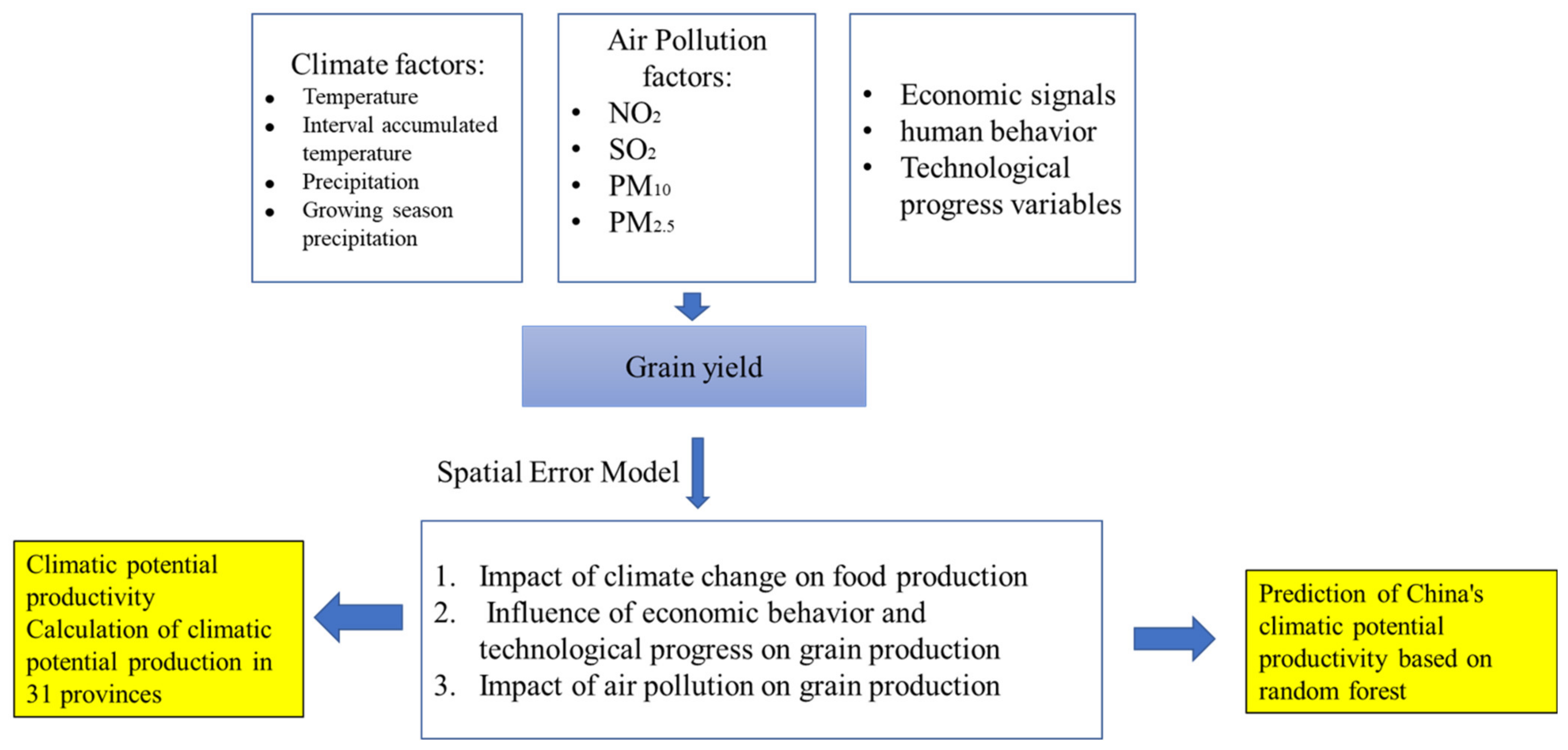
China is one of the world’s largest countries in terms of population as well as grain production. As such, China’s grain production and sales are of great importance to world food security [42]. However, both agronomy and economics have disciplinary limitations in the study of food production. They have their own characteristics in terms of research perspectives, contents, and methods [49]. Different prediction methods and research processes will lead to different evaluation results, increasing the difficulty in decision-making [50]. Therefore, we establish a framework (Figure 2) to link the causality between grain yield, climate factors, and air pollution factors.

The marginal contribution of this paper lies in the use of economic models to study agricultural problems. We use spatial error models to measure the impact of climate change and air pollution on food production, and this article measures the potential grain production with the impact of climate change and air pollution.

According to this framework, the two questions to be addressed in this study are:

• How do climate change and air pollution affect grain production in 31 provinces of China?
• How will China’s food production potential change in the context of climate change?

According to the research questions, the main objective of this research is to investigate the impact of climate change and air pollution on food security, as well as the role of economic behavior and technical factors in food production.

In order to achieve the main objectives, we use the spatial error model to test the impact of climate factors on grain production and use the mixed effect model to analyze the impact of seasonal precipitation and air pollution on grain production in 31 provinces. We further investigate the impact of climate change and air pollution on grain climate production potential and use the random forest model to predict grain production potential.

The remaining of the article consists of the following parts. Section 2 gives a brief overview of spatial error models, and discusses mixed effect models, food climate production potential models, and random forests. Section 3 describes the study area and data and defines variables. The results are given in Section 4, the impacts are discussed in Section 5, and the conclusions and shortcomings of the study are outlined in Section 6.

2. Methods

2.1. Panel Spatial Error Model

Based on Cobb–Douglas production function, a panel spatial error model (SEM) is established. This was performed after referring to existing literature pertaining to the setting of variables [51]:

$$Y_{p,t}={\beta }_1{X}_1+{\beta }_2{X}_2+\gamma C_{p,t}+\mu A_{p,t}+S_{p,t}+f_p(t)+{\epsilon }_{p,t}$$

(1)

In Formula (1), p represents province, t represents year, and $Y_{p,t}$ refers to the yield of grain crops in province p.

$X_1$ represents the impact of economic signals and $X_2$ represents human behavior on food yield. ${\beta }_{\mathrm{i}}$ is the dependence of output on economic signals and human behavior.

Also, ${\mathrm{C}}_{p,t}$ reflects the effect of climate factors on grain production.

$\gamma$ is the dependence of yield on climate variables. $A_{p,t}$ represents the impact of air pollution emissions on grain production.

$S_p$ is the area fixed effect, which is used to control for factors, such as elevation and soil, that do not change over time [21]; $f_p(t)$ is a time fixed effect explain the differences between provinces over time. The other influences in Equation (1) that are not captured by the independent variable are set as residual terms ${\epsilon }_{p,t}$. Examples include agricultural news, soil quality, farming systems, agricultural policies, regional natural disasters and regional ozone levels.

$${\epsilon }_{r,t}=\rho {\displaystyle \sum _p{W}_{p,t}{\epsilon }_{p,t}}+{\eta }_{p,t}$$

(2)

In order to compensate for potential omitted variables, this study assumes that a spatial correlation exists between provinces. The residual ${\epsilon }_{p,t}$ of adjacent provinces is used to explain the residual of a specific province [41]. In Equation (2) $W_{p,t}$ is a spatial weighted matrix, which defines the range of spatial correlation effects. This study uses a spatial contiguity matrix to reflect the spatial correlation of the sample. We assume that spatially correlated effects exist between adjacent provinces, but not exist between non-adjacent provinces. The degree of spatial correlation between adjacent provinces is reflected by the estimation coefficient ρ.

Formulas (1) and (2) constitute the panel spatial error model of this study, where ${\eta }_{p,t}$ is the true residual of the empirical model after the spatial correlation of the residual (${\epsilon }_{r,t}$) is removed.

2.2. Climatic Potential Productivity

The marginal effect of climate factors on grain yield can be obtained by using the panel spatial error model, that is, the coefficient estimates of ${\beta }_0$ and ${\beta }_1$.

Based on the determination of the marginal impact of climate factors on grain yields [52,53,54], the change of climatic productivity potential in China, which is a further explanation of the impact of climate change on grain production in China, must be further calculated.

Agriculture is greatly affected by climate elements, and climate change is a process of the overall changes in all factors [55]. Under the condition that nutrients remain appropriate, the upper limit of crop yield, which is jointly determined by sunlight, temperature, and water, is the climatic productivity potential [56].

Grain production is an important link in ensuring food security. As such, grasping the changing patterns of potential climatic productivity is crucial to ensuring national and even global food security [57,58,59,60].

Common models used to calculate potential climatic productivity include the Thorthwaite Memorial model [61,62,63,64], the Miami model [65,66], and the GAEZ model [67,68].

Temperature and precipitation are important climatic factors governing crop growth. The Miami model was used to separately calculate the production potential of temperature and precipitation. The formulae are as follows:

$$Y_t=\raisebox{1ex}{$3000$}\!\left/ \!\raisebox{-1ex}{$1+e^{1.315-0.119t}$}\right.$$

(3)

$$Y_r=3000\times (1-e^{-0.00664t})$$

(4)

In Formulas (3) and (4), t indicates the average annual temperature in degrees Celsius (°C); r indicates the annual precipitation in mm, and

$Y_t$ and $Y_r$ denote the production potential determined by annual average temperature and annual precipitation, respectively (kg/hm²/year).

Based on the relationship between evapotranspiration, temperature, precipitation, and crops, the Thorthwaite memorial model is used to calculate the climatic production potential for grain. The formula is as follows:

$$Y_e=3000\times \left[1-e^{-0.0009695\left(V-20\right)}\right]$$

(5)

$$V=1.5\mathrm{R}/{[1+{(1.05R/L)}^2]}^{1/2}V={\raisebox{1ex}{$1.5R$}\!\left/ \!\raisebox{-1ex}{$\left[1+{(1.05R/L)}^2\right]$}\right.}^{1/2}$$

(6)

$$L=300+25T+0.5T^3$$

(7)

In the above equation, V represents the average annual distillation (unit: mm); R represents the average annual precipitation (unit: mm); L represents the maximum annual evaporation (unit: mm); and $Y_e$ represents climatic productivity potential, calculated using evapotranspiration (unit: kg/hm²/year).

2.3. Random Forests

Breiman developed the random forests (RF) method in 2001 as an extension of the Bagging classification tree. The RF method was designed to improve the accuracy of predictions or regression [69]. In addition to improving the accuracy of classification or regression, RF provides a measure of the importance of variables (characteristics) for each candidate predictor. Each RF classifier is an ensemble classifier that uses a set of classification and regression trees for prediction and simulation. The RF algorithm is widely used in the field of classification, employing remote sensing images and pattern recognition in artificial intelligence [70,71,72]. The robustness and reliability of the RF model make it a desirable methodology for agricultural product prediction [73,74,75,76].

In the RF model, the number of decision trees and the number of variables to select and test should be predefined [72]. Based on the panel spatial error model, the Thorthwaite Memorial model and Miami model are combined to calculate the potential climatic production of grain in China. Furthermore, the random forest model is used to predict the potential climatic production.

3. Study Area and Data

3.1. Study Area

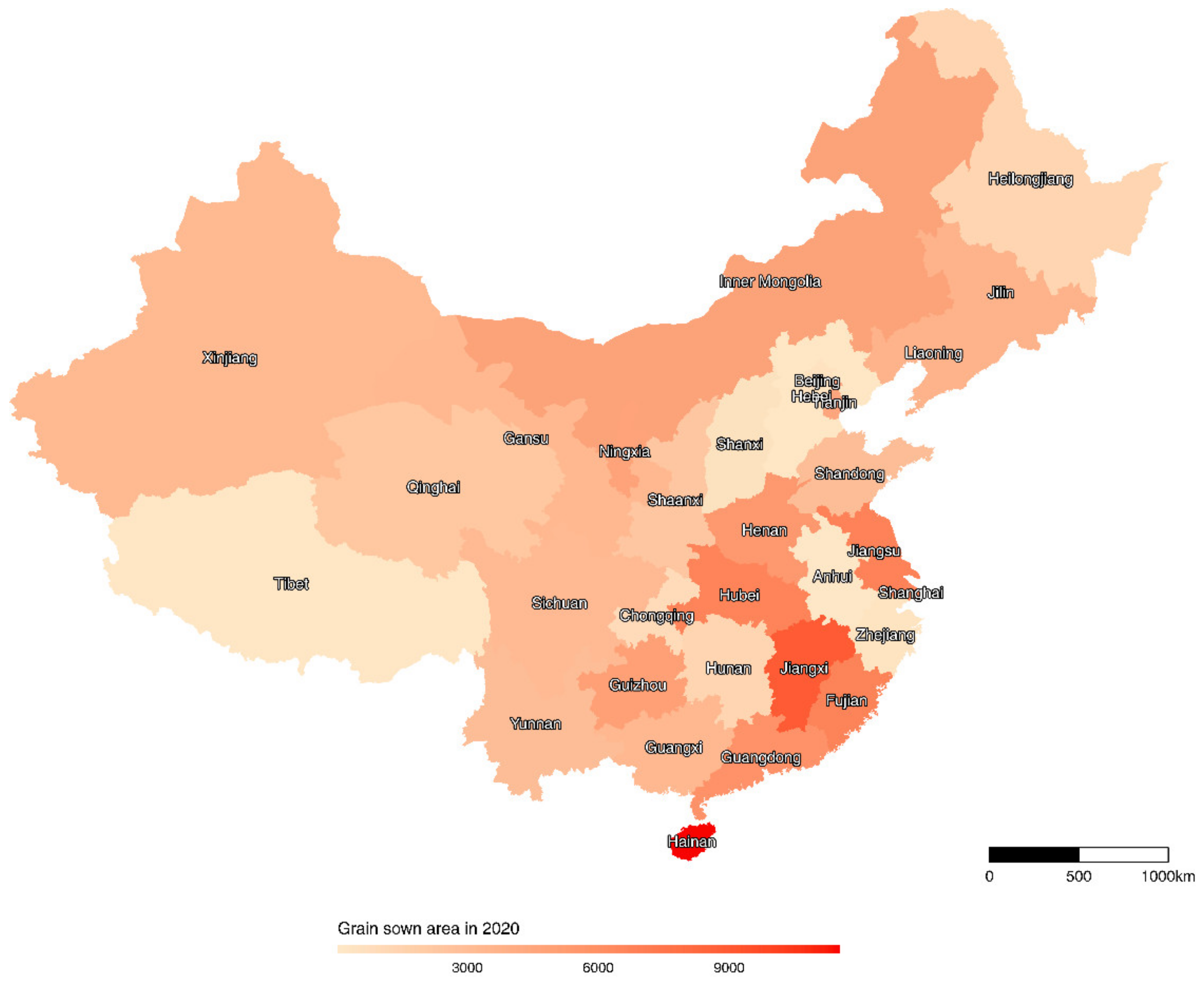
A total of 31 provincial units (hereafter referred to as provinces, including provinces, autonomous regions, and municipalities directly under the central government) are included in the study due to the significant differences in natural resource endowments between different regions of China. (Figure 3,

Table A2. Name of 31 provinces.

Name	Name	Name
Beijing	Zhejiang	Hainan
Tianjing	Anhui	Chongqing
Hebei	Fujian	Sichuan
Shanxi	Jiangxi	Guizhou
Inner Mongoria	Shandong	Yunnan
Liaoning	Henan	Tibet
Jilin	Hubei	Shaanxi
Heilongjiang	Hunan	Gansu
Shanghai	Guangdong	Qinghai
Jiangsu	Guangxi

).

3.2. Data Resources

Data used in this study include climate data, food crop growth cycle data, socio-economic statistics, and variables constructed in this research.

Climatic data: the data used in this study are panel data (from 2003 to 2020) of 31 provinces in mainland China. Meteorological observations covering the whole of China are used in this study. Climate data from the National Oceanic and Atmospheric Administration are available to download (https://www.ncei.noaa.gov/data/global-historical-climatology-network-daily (accessed on 6 June 2022)). The daily meteorological data used in this study include daily precipitation, average maximum temperature, average minimum temperature, rainfall, and sunshine duration. After data check and comparison, 226 meteorological stations in 31 provinces with stable observation data are selected for this study. An ANUSPLIN interpolation model is used to interpolate the data of meteorological stations [2,10]. This model is based on a smooth spline function considering the influence of terrain and other factors. Therefore, the accuracy of this model is higher than that of ordinary interpolation methods.

Grain crop growth cycle data: due to the wide variation in geographical climate, soils, grain crop varieties, and grain farming systems in China’s 31 provinces, the growth cycles and maturity systems of grain crops vary from region to region. Therefore, the “Provincial Agricultural Time Database” provided by the Department of Crop Production of the Ministry of Agriculture and Rural Affairs, PRC (http://www.zzys.moa.gov.cn/ (accessed on 6 June 2022)) is used to obtain the detailed time points of sowing, growth, development, and harvest of major crops in 31 provinces. The data are extremely accurate with regard to the months and seasons of each growth stage of crops. The total precipitation and sunshine duration during the growth cycle were collected according to the growth cycle of food crops. During the research period (2003–2020), the growth cycles of the grain crops in all 31 provinces were comprehensively recorded, providing key information for this study. The average monthly precipitation in the growing season is calculated based on the daily precipitation data to investigate the relationship between climate factors and yield per unit area during the growth cycle of grain crops.

Socio-economic statistics: the socio-economic data used in this study are mainly from the National Bureau of Statistics of China (http://www.stats.gov.cn/english/Statisticaldata/AnnualData/ (accessed on 6 June 2022)) and the China Statistical Yearbooks (1949–2021). The statistical results show that the main food crops in China are corn, wheat, and rice.

Data on air pollution: Information on annual average concentrations of SO₂, NO₂, PM₁₀, and PM_2.5 was collected for the period 2003–2020. These data are obtained from China’s Environmental Yearbooks (1949–2021). For missing data, we supplement this main dataset with the information collected manually from provincial statistical yearbooks, government reports, and bulletins. We obtained daily real-time data in 2020 at China Environmental Monitoring Station. (http://www.cnemc.cn/sssj/ (accessed on 6 June 2022)).

3.3. Data of Constructed Variables

Interval accumulated temperature variable: one of the manifestations of climate change is global warming. Therefore, a key variable was set up to establish the relationship between temperature and grain yield per unit area. Agronomy generally employs accumulated temperature indicators to measure the amount of heat absorbed by food crops during their growth cycle. The effect of temperature on the growth and development of food crops is reflected in both the intensity and duration of the action of the accumulated temperature [49]. The accumulated temperature is also widely used in empirical studies in the field of economics [50]. This study draws on previous research, dividing the temperature into exhaustive successive temperature bands [51]. Interval accumulation temperatures are calculated for every 5 °C temperature interval in the 0–40 °C range (IATD 0–5 °C, IATD 5–10 °C, IATD 10–15 °C, IATD 15–20 °C, IATD 20–25 °C, IATD 25–30 °C, IATD 30–35 °C, IATD 35–40 °C). Through the marginal effects of interval accumulation temperatures, a mapping between the corresponding temperature levels and grain yields is indirectly established.

When using a panel spatial error model, the effects of all IATD variables on grain yield were empirically tested. The effective temperature range for crop growth was identified, as well as the harmful temperature range and the inflection point of the marginal effect of temperature on grain yield.

Proxy variables of economic signals: to construct the economic signal proxy variable, the ratio of the crop production price indices with a lag period and the agricultural production means price indices of the current period were used to measure the income from crop cultivation. Higher ratios indicate greater returns from farming [47]. In particular, price data for grain crops were obtained from the National Bureau of Statistics database, including the Agricultural Production Price indices (APPI) of 31 provinces of China and the price indices of agricultural means of production (AMPi). The APPI reflects the relative trend and magnitude of changes in the prices of agricultural products sold by agricultural producers in each province each year. The AMPi is the relative number that reflects the trend and degree of the price changes of agricultural means of production in each province. In order to construct a proxy variable for human behavior, the effective irrigation ratio (EIR) was used to represent people’s behavioral adjustment to changes in climate conditions. In this study, EIR is the irrigated area divided by the cultivated area [44], and the irrigated area includes both irrigated and drained areas, with no distinction between the two, which reflects human behavior in regulating climate elements. In

Table 1. Descriptive statistical analysis of variables between 2003–2020.

Variables	Label	Mean	Std. Dev.
Dependent Variable
Grain yield per unit (kg/hm2)	Yields	5033.4	1010.03
Climate Variable
Extremely cold (Accumulated days)	CTD −0 °C	46.28	51.72
Interval accumulated temperature 0–5 °C (Accumulated days)	IATD 0–5 °C	33.65	19.51
Interval accumulated temperature 5–10 °C (Accumulated days)	IATD 5–10 °C	45.35	18.62
Interval accumulated temperature 10–15 °C (Accumulated days)	IATD 10–15 °C	50.12	18.2
Interval accumulated temperature 15–20 °C (Accumulated days)	IATD 15–20 °C	59.97	20.55
Interval accumulated temperature 20–25 °C (Accumulated days)	IATD 20–25 °C	65.91	22.16
Interval accumulated temperature 25–30 °C (Accumulated days)	IATD 25–30 °C	52.35	41.62
Interval accumulated temperature 30–35 °C (Accumulated days)	IATD 30–35 °C	10.72	14.43
Extremely hot (Accumulated days)	EHD 40 °C+	0.04	0.29
Effective accumulated temperature (Degrees Centigrade)	EAT	4202.194	1945.896
Active accumulated temperature (Degrees Centigrade)	AAT	2177.124	1206.035
Precipitation (mm)	PRE	920.28	449.18
Annual Sunshine Hours (Hours)	ASH	2453.253	705.14
Economic signals Variable
Cost-benefit ratio (%)	CBR	1.02	0.1
Effective irrigation ratio (%)	EIR	0.76	0.52
Technological progress Variable
Total power of agricultural machinery (kw/hm2)	TPAM	9.71	5.42
Year-end ownership of farmland infrastructure machinery (10,000 sets)	YOFIM	1.2	1.5
Air pollution Variable
Nitrogen dioxide (mg/m3)	NO2	41.01	12.01
Sulfur dioxide (mg/m3)	SO2	35.06	23.09
Inhalable particulate matter PM 2.5 (mg/m3)	PM 2.5	46.18	18.28
Inhalable particulate matter PM 10 (mg/m3)	PM 10	94.96	32.43

Note: In the method and result sections, these variables are transformed to log forms.

, the average EIR for China between 2003 and 2020 is 0.76. That means that the effective irrigation area of grain cultivated land accounts for 76% of the total sown area

The data used for EIR are from the National Bureau of Statistics database (http://data.stats.gov.cn (accessed on 6 June 2022)).

This study used the year-end possession of agricultural machines (set) and the general power of agricultural machines per hectare (kilowatts/hm²) in 31 provinces as proxy Technological progress variables. The total power of agricultural machinery refers to the sum of the rated power of all agricultural machinery power. We calculated the total power of agricultural machinery required for grain sowing per hectare.

Table 1 shows all the variables used in the empirical analysis section of this study and their descriptive statistical results. During the growth cycle, the interval accumulated temperature of grain crops was concentrated between 15 °C and 30 °C (interval accumulated temperature > 10 days), with an average of 2453.253 h of sunshine.

4. Results

4.1. Estimation Results and Interpretation

The Moran index and the spatial adjacency matrix (W) were used to verify the spatial correlation of the samples. If the coefficient value of the Moran index is significant, this indicates that a correlation exists between the sample provinces in terms of grain production.

Table 2. Results of correlation tests for variables.

Test Coefficient	n = 31
Moran’s-I	0.685 *
LM test	2403.331 ***
LR test	113.81 *
Wald’s test	57.64 *
Hausman test	25.34 **

Note: Significance denoted by *** p < 0.01, ** p < 0.05, and * p < 0.1. Furthermore, H0: Difference in coefficients is not systematic chi²(16) = 25.34, Prob ≥ chi² = 0.0166.

illustrates the high spatial correlation among the 31 samples.

In order to verify whether or not the spatial error effect and spatial lag effect existed in the overall panel data, an LM test, LR test, and Wald’s test are conducted in SEM, and the results are shown in Table 2. All tests consistently showed that a significant spatial correlation existed between the samples. The traditional panel fixed effects model (Equation (1)) is insufficient to deal with spatial correlation. The model’s estimation results are not only biased, but they also significantly overestimate the significance level of variables [41]. This bias essentially stems from the omission of spatial elements. Therefore, there is a need to introduce spatial econometric empirical methods for analysis purposes.

The Hausman test is used to verify whether the spatial error model is a fixed effects model or a random effect model. Table 2 shows the results of the Hausman test. According to the test results (p = 0.0166), the fixed effect model would be a more appropriate choice to estimate the selected variables.

4.2. Impact of Climate Change on Food Production

Based on the settings of the panel spatial error model Equations (1) and (2), we investigated the effects of climatic factors on grain yields in China. The obtained regression results are shown in

Table 3. Regression results of spatial error model.

Variables	Equation (1)	Equation (2)	Equation (3)
CTD−0 °C	−0.0818 *** (0.098)	−1.811 *** (0.058)	−0.77 *** (−1.45)
IATD 0–5 °C	0.00005 *** (0.0946)	−1.448 *** (0.086)	−0.195 *** (0.549)
IATD 5–10 °C	−0.0001 *** (0.0835)	−4.355 *** (0.073)	−0.6 *** (0.243)
IATD 10–15 °C	−4.51 ** (0.066)	−3.289 ** (0.0583)	−0.763 *** (0.026)
IATD 15–20 °C	−0.00037 *** (0.083)	−0.001 *** (0.0613)	−1.171 *** (0.024)
IATD 20–25 °C	−0.0005 ** (0.054)	0.002 *** (0.0814)	−1.121 *** (0.0262)
IATD 25–30 °C	−0.0004 *** (0.058)	1.213 *** (0.0019)	−0.9 *** (0.003)
IATD 30–35 °C	−0.0003 ** (0.066)	−4.72 *** (0.0731)	−0.839 *** (0.006)
EHD 40 °C+	−0.001 (0.149)	−13.54 (0.052)	−0.347 *** (0.072)
EFT	−0.0003 (0.069)	0.036 (0.001)	0.197 *** (0.07)
AAT	−0.0001 (0.027)	0.0019 (0.001)	−0.31 *** (0.075)
PRE	0.009 (0.263)	0.103 (0.207)	0.06 * (0.624)
ASH	0.0001 * (0.061)	1.174 * (0.046)	0.179 *** (0.034)
TPAM		0.0016 ** (0.0983)	0.18 *** (0.0007)
CBR		106.9 *** (0.001)	−2.16 *** (0.163)
EIR		0.004 (0.202)	1.12 *** (0.071)
YOFIM		0.0363471 *** (0.001)	0.004 *** (−0.39)
log (NO2)			−0.0066 *** (0.1691)
log (SO2)			0.019 * (0.009)
log (PM10)			−0.05 * (0.0023)
log (PM2.5)			−0.031 *** (0.0232)
Observation	527	527	527
Rho (ρ)	0.78 ***	0.177 ***	0.6235 ***
Lambda (λ)	0.3848 ***	0.6359 ***	0.486 ***
Log likelihood	3675.16	3373.34	3643.98

Note: p-values are in parentheses; *** denotes 1% level of significance; ** denotes 5% level of significance, and * denotes 10%.

. Equation (1) only includes all climate variables, while Equation (2) further incorporates the proxy variables of economic signals and human behavior, namely price ratio, and irrigation ratio, respectively. Air pollution variables are added to Equation (3).

The significance and estimated coefficients of the independent variables of Equations (1)–(3) tend to be consistent. These are essentially robustness tests for each other.

Extreme weather (CTD −0 °C and HDD 40 °C) significantly contributed to reduced grain yields during the study period. According to the statistics released by the Ministry of Emergency Management of the People’s Republic of China, during the period from 2003 to 2020, the average frequency of frost damage in China was 4.13. During the same period, the average reduction in grain yields in China due to frost damage was 0.352 kg/hm²–7.52 kg/hm². Higher temperatures are also unsuitable for grain yield. During the study period, HHD 40 °C had a significant negative effect on grain yield, with each unit increase in temperature resulting in a 13.54968 kg/hm² reduction in grain yield.

An inverted U-shaped non-linear relationship exists between temperature and grain yields. The regression results show that accumulated temperatures below 20 °C and above 30 °C both lead to reduced grain yields. This result shows an inverted U-shaped non-linear relationship between temperature levels and grain yields, with an increasing and then decreasing trend. In addition, the damage to grain yields from hot weather far exceeds that of low temperatures. Each additional day of temperature in the 0–5 °C range (IATD 0–5 °C) will result in an average reduction in grain yield of 1.448944 kg/hm². The grain yield decreased by 4.355178 kg/hm² on average when the temperature increased to 30–35 °C (IATD 0–5 °C). As a result of global warming, climate change is mainly manifested in higher average temperatures, and the accumulated temperature of the high-temperature range in the future is bound to increase cumulatively. This will almost certainly lead to reduced grain production in China. Combined with Table 1, both effective accumulated temperature (4202.194 °C) and active accumulated temperature (2177.124 °C) have a positive impact on grain yield. Each 1 °C increase in effective cumulative temperature leads to a 0.0363471 kg/hm² increase in grain yield; each 1 °C increase in active cumulative temperature leads to an increased grain yield of 0.00000972 kg/hm². Sunshine duration was positively correlated with grain yield during the study period, but precipitation (PRE) was not significantly correlated with grain yield (p = 0.207 < 0.05).

Based on the analysis of climate change and food production, we analyzed the impact of sub-seasonal average changes in precipitation on changes in food production (see Appendix A 

Table A1. Further analysis of the impact of seasonal precipitation on Grain Yield.

	Con.	t Value
spring	0.184 *	1.33
summer	0.558	0.58
autumn	−0.906	−0.118
winter	−0.575	−0.561
log(spring)	0.703 *	0.346
log(summer)	0.575 *	0.525
log(autumn)	0.433	0.563
log(winter)	−0.006	0.785
Observations	527	527
Log Likelihood	589.031	605.473
AIC	162.062	194.945
BIC	127.925	160.808

Note: * p < 0.1.

). We used seasonally averaged weather variables in the model rather than monthly variables to avoid too many predictor variables, which could lead to overfitting. The four seasons were defined as autumn (September–November), winter (December–February), spring (March–May), and summer (June–August). The results of the panel data mixed-effects model estimates indicate that the effect of spring precipitation variation on grain production in China is significant, with a p-value greater than 10%, summer precipitation is significantly associated with production in grain yield, with an estimated elasticity coefficient of 2.52 (significant at the 1% level) and no significant effect of changes in winter and autumn precipitation on grain yield.

4.3. Influence of Economic Behavior and Technological Progress on Grain Production

The cost-benefit ratio (CBR) of grain has a significant impact on grain yield (p = 0.001 < 0.005). Specifically, each 1% increase in the CBR led to a 106.9 kg/hm² increase in grain yield.

When growing food, farmers’ consideration of expected returns and costs significantly affects crop yields. The effective irrigation ratio (EIR), however, had no significant effect on grain yield (p = 0.202 > 0.1).

TPAM had no significant influence on grain yield per unit area (p = 0.0983 < 0.05), but YOFIM had a positive correlation with grain yield per unit area (p = 0.01 < 0.05). The development of modern agricultural science and technology has improved agricultural planting technology and grain yield to a certain extent. Each increase in farmland capital construction machinery at the end of the year will lead to an increase in grain yield of 0.0363471 kg/hm².

4.4. Impact of Air Pollution on Grain Production

From the model estimation results (Table 3), the estimated elasticity coefficient for NO₂ is −0.0066 (significant at the 1% level), and the estimation of Equation (3) shows an estimated elasticity coefficient for SO₂ of 0.019 (significant at the 1% level), the estimated elasticity coefficient for PM₁₀ is −0.05, and the estimated elasticity coefficient for PM_2.5 is −0.031. Controlling for other influencing factors, an average increase of 1% in PM 2.5 is associated with a decrease in grain yield of 0.031 kg/hm². This shows that the effect of air pollution variables on food production is significant and varies in magnitude depending on the variable.

When all the variables are introduced in the model (Table 3), The coefficient estimates for the EIR are 1.12 (p = 0.0101 < 0.01). The increase in EIR favors higher levels of grain production, controlling for other influencing factors. The Coefficient estimates for YOFIM are 0.004 (p < 0.1). This partly reflects the contribution of technical inputs in irrigation and agricultural machinery to the increase in food production. The coefficient estimates for climate change are decreasing as other variables are continuously added. This suggests that controlling for other factors, human economic behavior and the level of agricultural mechanization can mitigate the negative effects of climate change, air pollution on food production.

4.5. Calculation of Climatic Potential Production in 31 Provinces

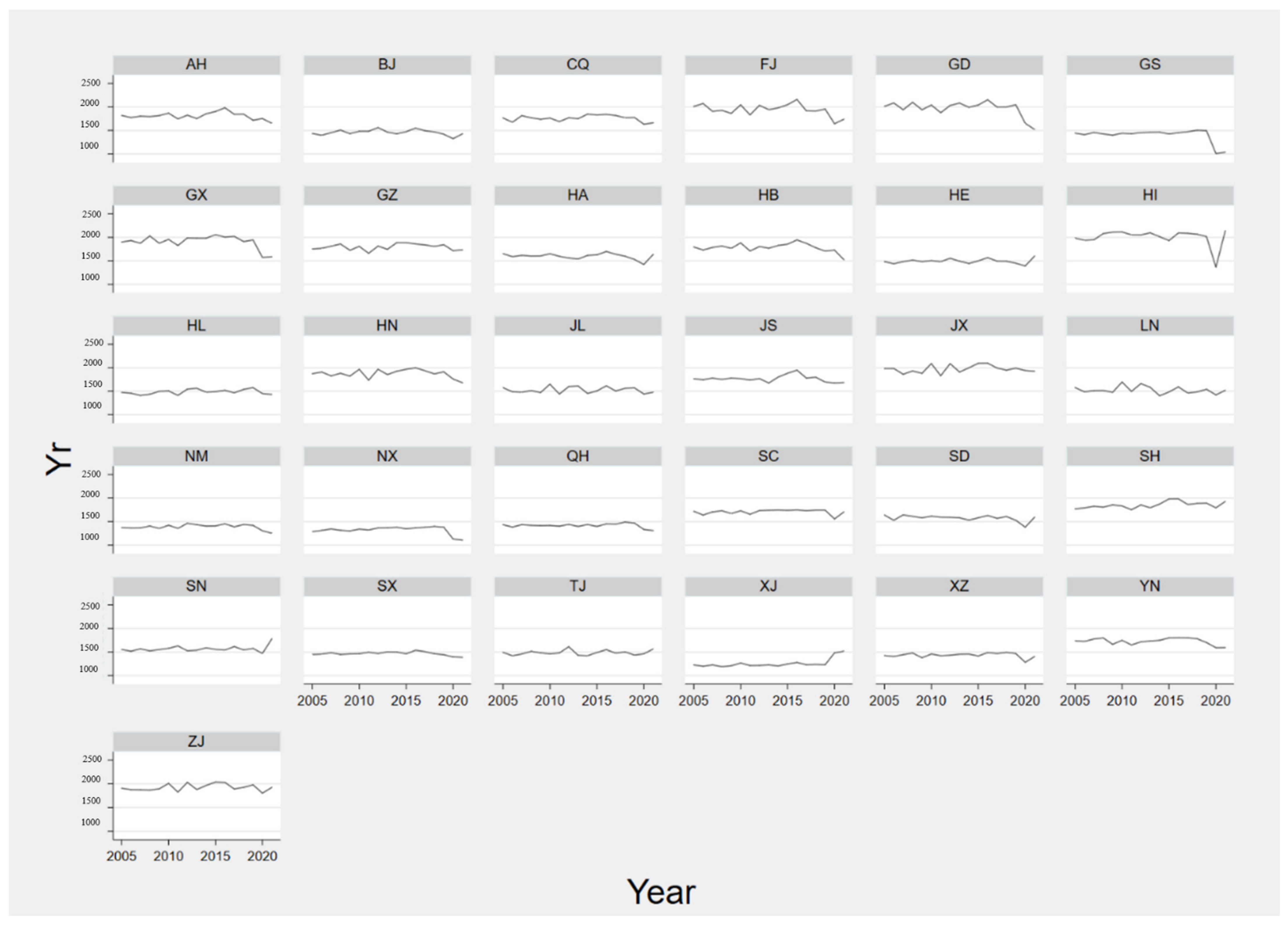
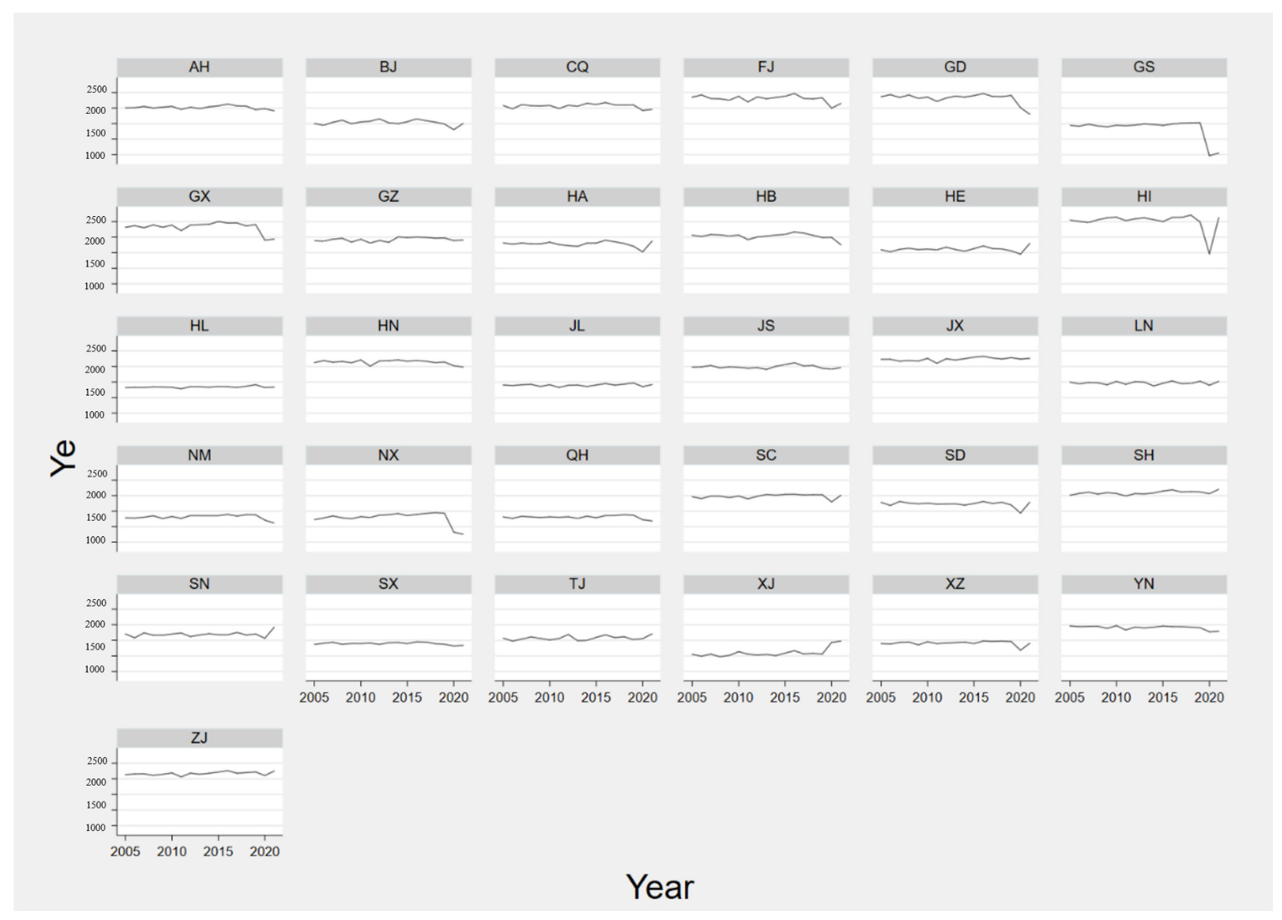
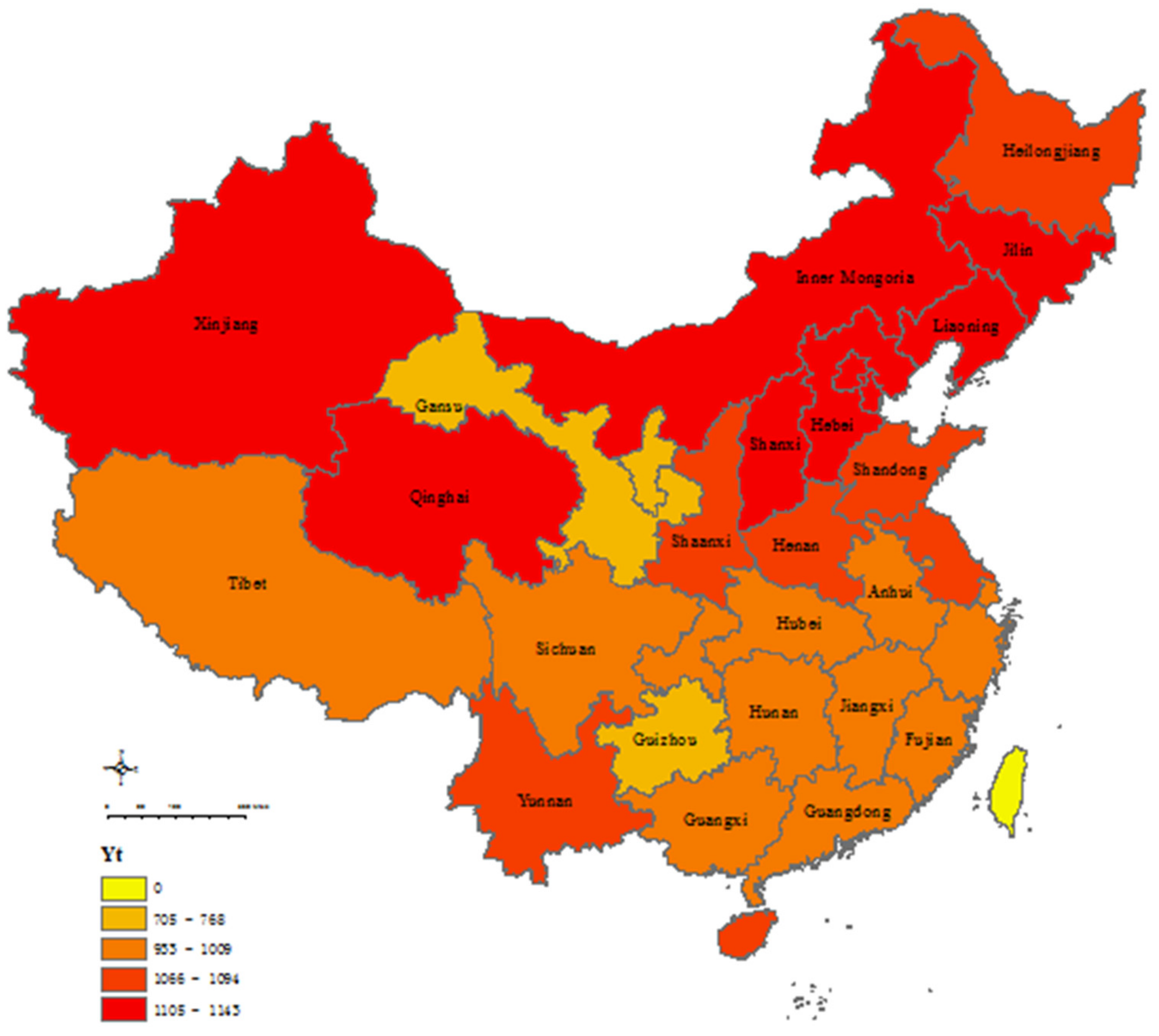
This study calculated the temperature production potential, precipitation production potential, and climate production potential for 31 provinces based on the Tharnthwaite Memorial model and the Miami model, respectively. Figure 4 shows the specific fluctuations in the average climatic production potential of grain crops in the 31 provinces. A graph of fluctuations in climatic productivity potential by province is shown in Appendix A, Figure A1, Figure A2 and Figure A3.

As shown in Figure 4, the fluctuation of productive climatic potential in 31 provinces in time is as follows:

• Temperature potential production Yt showed characteristics of minor fluctuations. Temperature production potential fluctuated more moderately from 2005–2021, generally at around 1787.87 kg/hm². Temperature production potential reached its maximum in 2007 and then began to decline significantly, reaching 2.83% in 2008. The potential picked up between 2017 and 2020, but the increase was limited.
• Precipitation production potential Y_r showed characteristics of fluctuation—decline—small rise. Precipitation production potential fluctuated significantly from 2005 to 2021; the difference between the maximum value and minimum value was 455.37 kg/hm². Fluctuations were more moderate from 2005 to 2009 and more volatile during the period 2016 to 2020. In 2016, precipitation production potential reached its maximum in the entire measurement period and then began to decline significantly.
• Distillation climate potential production (Ye) showed characteristics of minor fluctuations—fluctuating down. The overall climate production potential of distillation decreased by 2.91% from 2005 to 2021. The results also show that Ye fluctuated more in line with Yr, and after a small fluctuation, started to fluctuate downwards in 2020.

Taken together, the temporal evolutionary characteristics of the potential climatic production of the 31 sampled provinces show similarities to most research results from different regions and time periods [73,76,77].

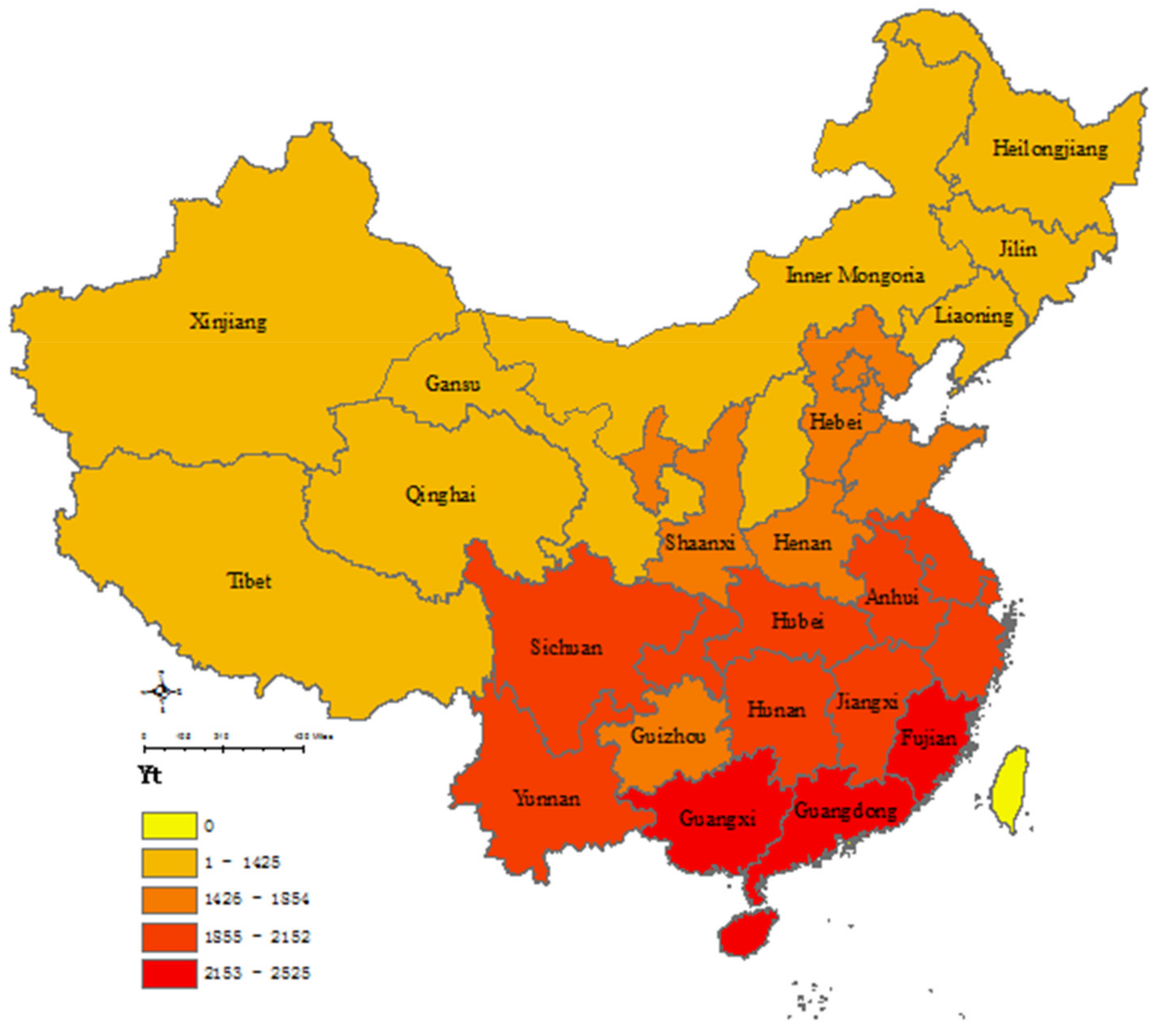
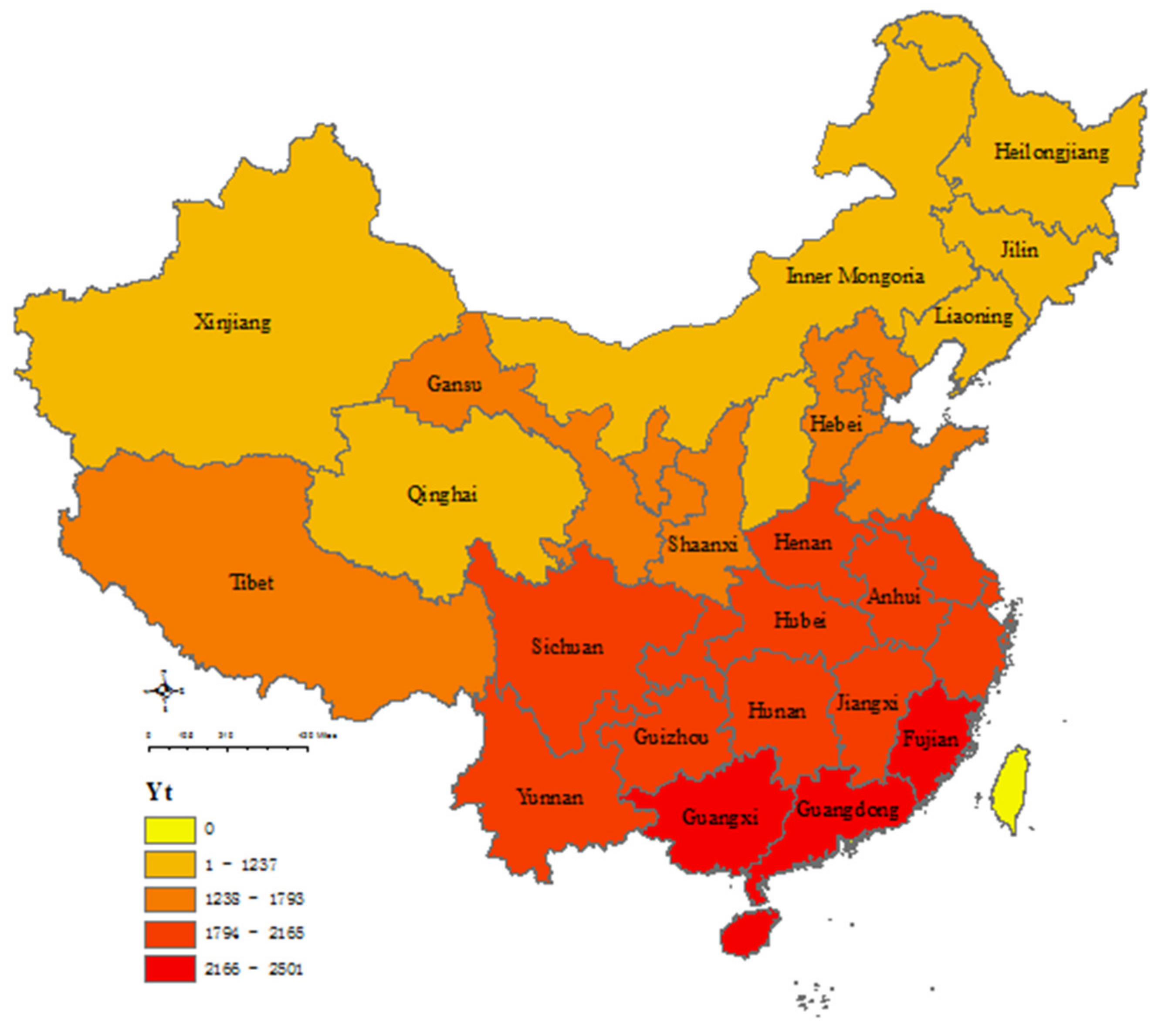
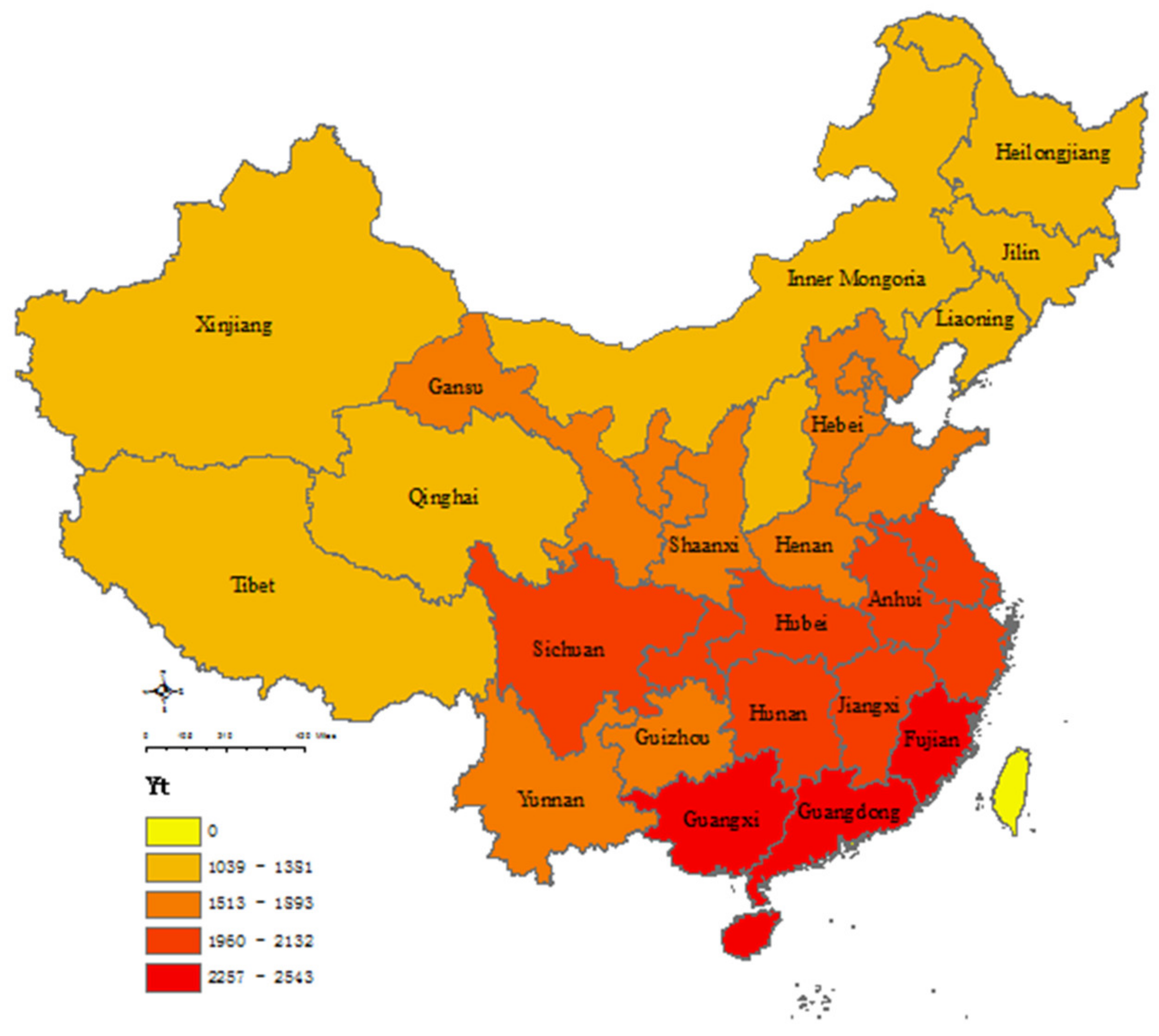
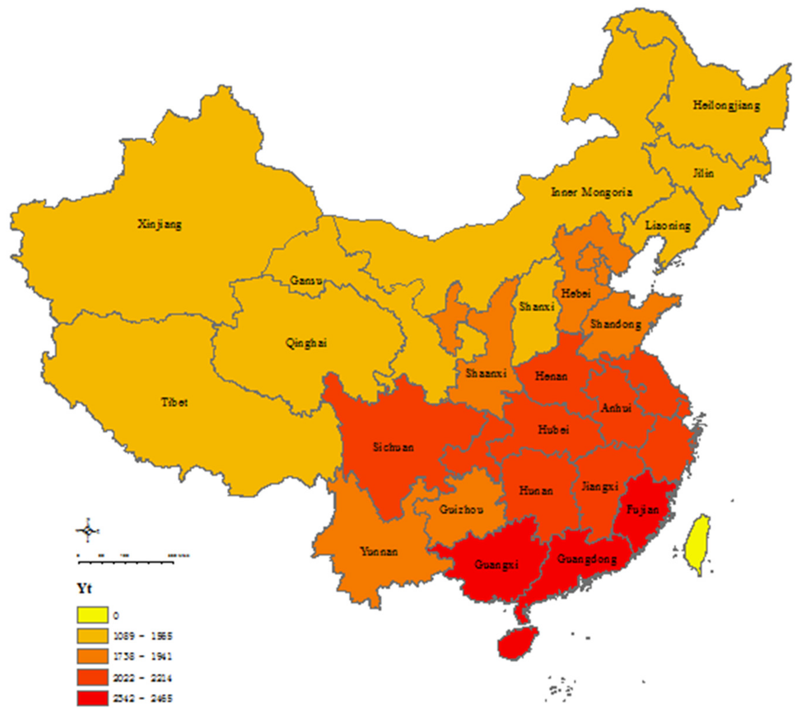
A further spatial interpolation was performed in ArcGIS 10.8, using the measurements as point data. The interpolation results of grain climate potential production for 2005, 2010, 2015 and 2021 are shown in Figure 5, Figure 6, Figure 7 and Figure 8.

The spatial variation characteristics of China’s grain climatic productivity potential can be seen from the spatial distribution of 31 provinces in Figure 5, Figure 6, Figure 7 and Figure 8.

The spatial distribution of grain climate potential productivity of 31 provinces decreased from southeast to northwest during the study period.

The average climatic production potential of the Pearl River Delta region, located in the tropical climates of Hainan, Guangdong, and Fujian Provinces, exceeded 1800 kg/hm².

However, China’s main grain production areas are mainly located in the plains of the middle and lower reaches of the Yangtze River and in the eastern Sichuan region. The predominantly subtropical monsoon climate in these areas is suitable for the cultivation of rice and other food crops. These areas are also an important commodity grain base in China.

China’s important commercial grain bases are concentrated in the Jiangsu and Anhui-Jianghuai regions, the Jianghan Plain in Hubei, the Dongting Lake Plain in Hunan, the Poyang Lake Plain in Jiangxi, and the Chengdu Plain in Sichuan. The average grain climate production potential in these regions is about 1600 kg/hm².

The main wheat-growing regions in China are located mainly in the temperate monsoon climate zone. The North China Plain, Northeast China Plain, Anning River Valley plain in southwest Sichuan Province, and the Hetao Plain in Inner Mongolia and its eastern region are the main wheat-growing regions. Most of the arable land in these areas is dryland and, therefore, suitable for the production of wheat, with an average climatic production potential of 900–1000 kg/hm².

The average annual climatic production potential is less than 700 kg/hm² in northwestern China, which includes such areas as the western desert of Inner Mongolia and the western Sichuan plateau. The same is true of the mountainous areas of northeastern China, including the Great Khingan Mountains, which are affected by light, temperature, and precipitation. The climatic and geographical conditions in these areas are relatively unfavorable for food production. The spatial distribution evolution of grain climatic productivity potential in China has three main characteristics:

• Less change occurs in areas with higher climate production potential. From 2005 to 2021, there was no change in the number of areas with an average climatic productivity potential above 1800 kg/hm² in China’s major grain-producing areas. There was also no change in the number of areas with high climatic productivity potential in non-grain producing areas, which were concentrated in Hainan and the Pearl River Delta.
• Areas with low climatic productivity potential are expanding. From 2005 to 2015, the areas with climatic productivity potential below 1000 kg/hm² were mainly in the western Sichuan plateau and western Inner Mongolia desert. However, between 2015 and 2021, areas with climate productivity potential below 1425 kg/hm² were expanding.
• The spatial difference in climate productivity potential in the middle region has shown a tendency to expand. We refer to the area with a climate production potential value of between 1400 kg/hm² and 2150 kg/hm² as the median region. From 2005 to 2021, the distribution range of the median region tended to expand. After 2015, the median zone gradually expanded and became concentrated in central Sichuan Province, southwards in Hebei Province and Hunan Province, and northwards in Hubei Province. The expansion of the median area weakened the spatial differences in the distribution of grain climatic potential productivity.

4.6. Prediction of China’s Climatic Potential Productivity Based on Random Forest

Compared to other machine learning methods (

Table 4. Evaluation metrics for various model applied to predict grain yields.

Model	r2 (0–1)	MSE (0–1)	MAE (0–1)
Random forest	0.9965	0.039	0.232
Linear regression	0.8894	0.416	0.214

Note: The closer the R² is to 1, the better the model fits. The closer the MAE and MSE values are to 0, the better the results are.

), RF models do not require multiple adjustments of parameters, are simple to set, and directly reflect the importance of indicator features [70,71]. We implemented RF in the Scikit-Learn library in Python [72]. A total of 1608 data were randomly selected as the training set, and 178 data were selected as the validation set.

We selected linear regression and RF for comparison to further validate the RF model. The coefficient of determination R², the mean absolute error (MAE), and the mean square error (MSE) were chosen to compare the predictions of the two models. The RF model has an MSE of 0.039 and an MAE of 0.232, which is lower than the linear regression (MSE = 0.416, MAE = 0.214). R2 = 0.9965, higher than predicted by linear regression (0.8894). This finding suggests that the model fits well and that the RF model can be used to predict climate production potential [73].

The results are shown in Figure 9. The predicted results differed significantly from the spatial distribution pattern of grain climatic productivity potential in China (Figure 5, Figure 6, Figure 7 and Figure 8). We believe that air quality affects climate production potential, and this is confirmed in the panel spatial error model. Other studies have also confirmed the relationship between air pollution and climate production potential [74,75,76,77].

Compared with the spatial distribution pattern of Grain climate productivity potential from 2003–2020 (Figure 5, Figure 6, Figure 7 and Figure 8), The overall food climate production potential of 31 provinces has declined. Air pollution can pose a threat to food production, and RF prediction results confirm that air pollution affects food climate production potential, leading to a decrease in the overall food climate production potential value.

Under the dual role of climate change and air pollution, the higher values of climatic production potential are concentrated in the northern regions. The climatic production potential values of the main food production bases are in the medium range, and the lower climatic production potential values are in Gansu, Ningxia, Inner Mongolia, the Qinghai-Tibet Plateau, and the Yunnan–Guizhou Plateau because these provinces are dominated by animal husbandry.

5. Discussion

Most existing literature [61,62,63,64,78,79,80,81] assesses the impact of climate change on agricultural production based on a particular region, which fails to consider the impact of human economic behavior. This study examines the impact of climate change on grain yields. Through a panel spatial error model analysis of climate factors and the calculation of China’s grain climate production potential, the following conclusions can be drawn:

First, extreme weather (CTD −0 °C and EHD 40 °C+) significantly reduces grain yield. Higher temperatures are not conducive to food production. The high-temperature weather variable (EHD 40 °C+) had a significant negative effect on grain yields. The results show that each unit increase in temperature will result in a reduction in grain yield of 13.54968 kg/hm². This is similar to the conclusion of other literatures [82,83,84], except that Tao [84] predicts that CO₂ will lead to a 2.8–11.7% decline in Wheat Productivity in 2020.

Second, an inverted U-shaped non-linear relationship exists between air temperature and grain yields. The regression results show that cumulative temperatures below 20 °C and above 30 °C both lead to reduced grain yields. Climate change due to global warming is mainly manifested in higher average temperatures. The inter-zone accumulation of temperature ranges in the future is bound to increase cumulatively, which in turn will lead to reduced grain production in China.

Third, when growing food, farmers’ consideration of expected returns and the costs of growing food significantly affect crop yields. Human interventions in food production (EIR) have no effect on food production (p = 0.202 > 0.1). However, a positive relationship was found between YOFIM and grain yields (p = 0.01 < 0.05). According to Chen (2021), this is because the development of modern agricultural science and technology has effectively improved agricultural planting technology and, to a certain extent, has improved grain output [48]. Each increase in YOFIM will result in an increase in grain yield of 0.0363471 kg/hm². In the long term, 37.9% of the short-term impact of climate change on total factor productivity in agriculture can be offset by agricultural machinery [48].

Fourth, under the combined action of climate factors, during the study period, the spatial structure of grain climate productivity potential in China showed an obvious step-like decline from southeast to northwest. The extreme value gap has widened further, with grain climate production potential in southeastern Jiangxi Province above 2000 kg/hm². In contrast, the climatic production potential of grain in Inner Mongolia and western Sichuan was below 1400 kg/hm². At the same time, the adjustment of the regional pattern intensified. The random forest model predictions validate this result. The model also predicted a good fit of 0.99, with good prediction results.

6. Conclusions

This study used the SEM to discuss the spatial impact of climate change and air pollution on grain production in China. We observed that climate change and air pollution have a significant impact on grain production. Global warming can lead to a reduction in food production. We have observed that SO₂, PM₁₀.PM_2.5 all have significant impacts on food production, with global warming leading to reduced food production.

Based on the assessment of potential climatic production for grain in China, we observed that the low-value areas of grain potential production are expanding while the high-value area is decreasing. This study presents Random Forest for efficiently predicting spatially and temporally explicit climate change and air pollution impacts on grain production potential. RF predicts climatic grain production potential to decline overall and the spatial distribution pattern of change.

There are a few limitations worth emphasizing in this article. We do not further decompose the impact mechanism of Agricultural Mechanization on agriculture. Future research needs to better understand its mechanism in eliminating the negative impact of climate change.

References

1. Asseng, S.; Ewert, F.; Rosenzweig, C.; Jones, J.W.; Hatfield, J.L.; Ruane, A.C.; Boote, K.; Thorburn, P.J.; Rötter, R.; Cammarano, D.; et al. Uncertainty in simulating wheat yields under climate change. Nat. Clim. Chang. 2013, 3, 827–832. [Google Scholar] [CrossRef] [Green Version]
2. Asseng, S.; Foster, I.; Turner, N.C. The impact of temperature variability on wheat yields. Glob. Chang. Biol. 2011, 17, 997–1012. [Google Scholar] [CrossRef]
3. Godfray, H.C.J.; Beddington, J.R.; Crute, I.R.; Haddad, L.; Lawrence, D.; Muir, J.F.; Pretty, J.; Robinson, S.; Thomas, S.M.; Toulmin, C. Food security: The challenge of feeding 9 billion people. Science 2010, 327, 812–818. [Google Scholar] [CrossRef] [PubMed] [Green Version]
4. Tilman, D.; Balzer, C.; Hill, J.; Befort, B.L. Global food demand and the sustainable intensification of agriculture. Proc. Natl. Acad. Sci. USA 2011, 108, 20260–20264. [Google Scholar] [CrossRef] [Green Version]
5. Piao, S.L.; Ciais, P.; Huang, Y.; Shen, Z.H.; Peng, S.S.; Li, J.S.; Zhou, L.P.; Liu, H.Y.; Ma, Y.C.; Ding, Y.H.; et al. The impacts of climate change on water resources and agriculture in China. Nature 2010, 467, 43–51. [Google Scholar] [CrossRef]
6. Lobell, D.B.; Schlenker, W.; Costa-Roberts, J. Climate trends and global crop production since 1980. Science 2011, 333, 616–620. [Google Scholar] [CrossRef] [Green Version]
7. Kuang, W.; Hu, Y.; Dai, X.; Song, X. Investigation of changes in water resources and grain production in China: Changing patterns and uncertainties. Theor. Appl. Climatol. 2015, 122, 557–565. [Google Scholar] [CrossRef]
8. Xiong, W.; Holman, I.; Lin, E.; Conway, D.; Jiang, J.; Xu, Y.; Li, Y. Climate change, water availability and future cereal production in China. Agric. Ecosyst. Environ. 2010, 135, 58–69. [Google Scholar] [CrossRef]
9. Guo, E.L.; Liu, X.P.; Zhang, J.Q.; Wang, Y.F.; Wang, C.L.; Wang, R.; Li, D.J. Assessing spatiotemporal variation of drought and its impact on maize yield in Northeast China. J. Hydrol. 2017, 553, 231–247. [Google Scholar] [CrossRef]
10. Holst, R.; Yu, X.; Grün, C. Climate Change, Risk and Grain Yields in China. J. Integr. Agric. 2013, 12, 1279–1291. [Google Scholar] [CrossRef]
11. Lobell David, B.; Burke Marshall, B.; Tebaldi, C.; Mastrandrea Michael, D.; Falcon Walter, P.; Naylor Rosamond, L. Prioritizing Climate Change Adaptation Needs for Food Security in 2030. Science 2008, 319, 607–610. [Google Scholar] [CrossRef] [PubMed]
12. Rosenzweig, C.; Elliott, J.; Deryng, D.; Ruane, A.C.; Müller, C.; Arneth, A.; Boote, K.J.; Folberth, C.; Glotter, M.; Khabarov, N.; et al. Assessing agricultural risks of climate change in the 21st century in a global gridded crop model intercomparison. Proc. Natl. Acad. Sci. USA 2014, 111, 3268–3273. [Google Scholar] [CrossRef] [PubMed] [Green Version]
13. Schmidhuber, J.; Tubiello, F.N. Global food security under climate change. Proc. Natl. Acad. Sci. USA 2007, 104, 19703–19708. [Google Scholar] [CrossRef] [Green Version]
14. Pittelkow, C.M.; Liang, X.Q.; Linquist, B.A.; van Groenigen, K.J.; Lee, J.; Lundy, M.E.; van Kessel, C. Productivity limits and potentials of the principles of conservation agriculture. Nature 2015, 517, 365–368. [Google Scholar] [CrossRef]
15. Miraglia, M.; Marvin, H.; Kleter, G.; Battilani, P.; Brera, C.; Coni, E.; Cubadda, F.; Croci, L.; De Santis, B.; Dekkers, S.; et al. Climate change and food safety: An emerging issue with special focus on Europe. Food Chem. Toxicol. 2009, 47, 1009–1021. [Google Scholar] [CrossRef] [PubMed]
16. Shi, W.J.; Tao, F.L. Spatio-temporal distributions of climate disasters and the response of wheat yields in China from 1983 to 2008. Nat. Hazards 2014, 74, 569–583. [Google Scholar] [CrossRef]
17. Wu, H.; Hou, W.; Qian, Z.H.; Hu, J.G. The research on the sensitivity of climate change in China in recent 50 years based on composite index. Acta Phys. Sin. 2012, 61, 562–571. [Google Scholar] [CrossRef]
18. Wang, B.; Hong, G.; Cui, C.Q.; Yu, H.; Murty, T. Comprehensive analysis on China’s National Climate Change Assessment Reports: Action and emphasis. Front. Eng. Manag. 2019, 6, 52–61. [Google Scholar] [CrossRef]
19. Shen, D.J. Climate change and water resources: Evidence and estimate in China. Curr. Sci. 2010, 98, 1063–1068. [Google Scholar]
20. Li, R.L.; Shu, G. Impacts of Climate Change on Agriculture and Adaptive Strategies in China. J. Integr. Agric. 2013, 12, 1402–1408. [Google Scholar] [CrossRef]
21. Chen, S.A.; Chen, X.G.; Xu, J.T. Impacts of climate change on agriculture: Evidence from China. J. Environ. Econ. Manag. 2016, 76, 105–124. [Google Scholar] [CrossRef]
22. Shi, W.J.; Tao, F.L.; Liu, J.Y. Changes in quantity and quality of cropland and the implications for grain production in the Huang-Huai-Hai Plain of China. Food Secur. 2013, 5, 69–82. [Google Scholar] [CrossRef]
23. Li, T.T.; Long, H.L.; Zhang, Y.N.; Tu, S.S.; Ge, D.Z.; Li, Y.R.; Hu, B.Q. Analysis of the spatial mismatch of grain production and farmland resources in China based on the potential crop rotation system. Land Use Policy 2017, 60, 26–36. [Google Scholar] [CrossRef]
24. Wang, C.Y.; Linderholm, H.W.; Song, Y.L.; Wang, F.; Liu, Y.J.; Tian, J.F.; Ren, G.Y. Impacts of Drought on Maize and Soybean Production in Northeast China During the Past Five Decades. Int. J. Environ. Res. Public Health 2020, 17, 2459. [Google Scholar] [CrossRef] [Green Version]
25. Yu, M.X.; Li, Q.F.; Hayes, M.J.; Svoboda, M.D.; Heim, R.R. Are droughts becoming more frequent or severe in China based on the Standardized Precipitation Evapotranspiration Index: 1951–2010? Int. J. Climatol. 2014, 34, 545–558. [Google Scholar] [CrossRef]
26. Shao, Y.; Dong, C.H. A review on East Asian dust storm climate, modelling and monitoring. Glob. Planet Chang. 2006, 52, 1–22. [Google Scholar] [CrossRef]
27. Shi, P.J.; Sun, S.; Wang, M.; Li, N.; Wang, J.A.; Jin, Y.Y.; Yin, W.X. Climate change regionalization in China (1961–2010). Sci. China Earth Sci. 2014, 57, 2676–2689. [Google Scholar] [CrossRef]
28. Tong, S.L.; Berry, H.L.; Ebi, K.; Hilary, B.; Hu, W.B.; Green, D.; Butler, C.D. Climate change, food, water and population health in China. Bull. World Health Organ. 2016, 94, 759–765. [Google Scholar] [CrossRef] [PubMed]
29. Chen, C.Q.; Lei, C.X.; Deng, A.X.; Qian, C.R.; Hoogmoed, W.; Zhang, W.J. Will higher minimum temperatures increase corn production in Northeast China? An analysis of historical data over 1965–2008. Agric. For. Meteorol. 2011, 151, 1580–1588. [Google Scholar] [CrossRef]
30. Yin, P.H.; Fang, X.Q.; Yun, Y.R. Regional differences of vulnerability of food security in China. J. Geogr. Sci. 2009, 19, 532–544. [Google Scholar] [CrossRef]
31. Feng, S.F.; Hao, Z.C. Quantifying likelihoods of extreme occurrences causing maize yield reduction at the global scale. Sci. Total Environ. 2020, 704, 135250. [Google Scholar] [CrossRef] [PubMed]
32. Zhang, L.L.; Zhang, Z.; Chen, Y.; Wei, X.; Song, X. Exposure, vulnerability, and adaptation of major maize-growing areas to extreme temperature. Nat. Hazards 2018, 91, 1257–1272. [Google Scholar] [CrossRef]
33. Wang, J.X.; Yang, Y.; Huang, J.K.; Adhikari, B. Adaptive irrigation measures in response to extreme weather events: Empirical evidence from the North China plain. Reg. Environ. Chang. 2019, 19, 1009–1022. [Google Scholar] [CrossRef]
34. Shi, W.J.; Wang, M.L.; Liu, Y.T. Crop yield and production responses to climate disasters in China. Sci. Total Environ. 2021, 750, 141147. [Google Scholar] [CrossRef]
35. Huang, J.; Lei, Y.D.; Zhang, F.M.; Hu, Z.H. Spatio-temporal analysis of meteorological disasters affecting rice, using multi-indices, in Jiangsu province, Southeast China. Food Secur. 2017, 9, 661–672. [Google Scholar] [CrossRef]
36. Guan, X.J.; Zang, Y.W.; Meng, Y.; Liu, Y.; Lv, H.; Yan, D.H. Study on spatiotemporal distribution characteristics of flood and drought disaster impacts on agriculture in China. Int. J. Disaster Risk Reduct. 2021, 64, 102504. [Google Scholar] [CrossRef]
37. Lawless, C.; Semenov, M.A. Assessing lead-time for predicting wheat growth using a crop simulation model. Agric. For. Meteorol. 2005, 135, 302–313. [Google Scholar] [CrossRef]
38. Singh, K.K.; Kalra, N. Simulating impact of climatic variability and extreme climatic events on crop production. Mausam 2016, 67, 113–130. [Google Scholar] [CrossRef]
39. You, L.Z.; Rosegrant, M.W.; Wood, S.; Sun, D.S. Impact of growing season temperature on wheat productivity in China. Agric. For. Meteorol. 2009, 149, 1009–1014. [Google Scholar] [CrossRef]
40. Xie, W.; Huang, J.K.; Wang, J.X.; Cui, Q.; Robertson, R.; Chen, K. Climate change impacts on China’s agriculture: The responses from market and trade. China Econ. Rev. 2020, 62, 101256. [Google Scholar] [CrossRef]
41. Schlenker, W.; Hanemann, W.M.; Fisher, A.C. The impact of global warming on US agriculture: An econometric analysis of optimal growing conditions. Rev. Econ. Stat. 2006, 88, 113–125. [Google Scholar] [CrossRef]
42. Yuan, W.P.; Liu, S.G.; Liu, W.; Zhao, S.Q.; Dong, W.J.; Tao, F.L.; Lin, H. Opportunistic Market-Driven Regional Shifts of Cropping Practices Reduce Food Production Capacity of China. Earths Future 2018, 6, 634–642. [Google Scholar] [CrossRef] [Green Version]
43. Yang, X.G.; Chen, F.; Lin, X.M.; Liu, Z.J.; Zhang, H.L.; Zhao, J.; Tang, H.J. Potential benefits of climate change for crop productivity in China. Agric. For. Meteorol. 2015, 208, 76–84. [Google Scholar] [CrossRef]
44. Deschenes, O.; Greenstone, M. The economic impacts of climate change: Evidence from agricultural output and random fluctuations in weather. Am. Econ. Rev. 2007, 97, 354–385. [Google Scholar] [CrossRef] [Green Version]
45. Nordhaus, W. Climate Change: The Ultimate Challenge for Economics. Am. Econ. Rev. 2019, 109, 1991–2014. [Google Scholar] [CrossRef]
46. Mendelsohn, R.; Nordhaus, W.D.; Shaw, D. The Impact of Global Warming on Agriculture: A Ricardian Analysis. Am. Econ. Rev. 1994, 84, 753–771. [Google Scholar] [CrossRef]
47. Welch, J.R.; Vincent, J.R.; Auffhammer, M.; Moya, P.F.; Dobermann, A.; Dawe, D. Rice yields in tropical/subtropical Asia exhibit large but opposing sensitivities to minimum and maximum temperatures. Proc. Natl. Acad. Sci. USA 2010, 107, 14562–14567. [Google Scholar] [CrossRef] [Green Version]
48. Chen, S.; Gong, B.L. Response and adaptation of agriculture to climate change: Evidence from China. J. Dev. Econ. 2021, 148, 102557. [Google Scholar] [CrossRef]
49. Baskerville, G.L.; Emin, P. Rapid Estimation of Heat Accumulation from Maximum and Minimum Temperatures. Ecology 1969, 50, 514–517. [Google Scholar] [CrossRef]
50. Chen, Y.; Zhang, Z.; Wang, P.; Song, X.; Wei, X.; Tao, F.L. Identifying the impact of multi-hazards on crop yield-A case for heat stress and dry stress on winter wheat yield in northern China. Eur. J. Agron. 2016, 73, 55–63. [Google Scholar] [CrossRef]
51. Schlenker, W.; Roberts, M.J. Nonlinear Temperature Effects Indicate Severe Damages to US Crop Yields under Climate Change. Proc. Natl. Acad. Sci. USA 2009, 106, 15594–15598. [Google Scholar] [CrossRef] [PubMed] [Green Version]
52. Vlachokostas, C.; Nastis, S.A.; Achillas, C.; Kalogeropoulos, K.; Karmiris, I.; Moussiopoulos, N.; Limperi, N. Economic damages of ozone air pollution to crops using combined air quality and GIS modelling. Atmos. Environ. 2010, 44, 3352–3361. [Google Scholar] [CrossRef]
53. Blandino, M.; Badeck, F.W.; Giordano, D.; Marti, A.; Rizza, F.; Scarpino, V.; Vaccino, P. Elevated CO2 Impact on Common Wheat (Triticum aestivum L.) Yield, Wholemeal Quality, and Sanitary Risk. J. Agric. Food Chem. 2020, 68, 10574–10585. [Google Scholar] [CrossRef] [PubMed]
54. De la Torre, D. Relative Yield Loss Calculations in Wheat due to Ozone Exposure. Sci. World J. 2010, 10, 103–115. [Google Scholar] [CrossRef] [PubMed] [Green Version]
55. Mola-Yudego, B. Regional Potential Yields of Short Rotation Willow Plantations on Agricultural Land in Northern Europe. Silva Fenn. 2010, 44, 63–76. [Google Scholar] [CrossRef] [Green Version]
56. Gonsamo, A.; Chen, J.M.; Lombardozzi, D. Global vegetation productivity response to climatic oscillations during the satellite era. Glob. Chang. Biol. 2016, 22, 3414–3426. [Google Scholar] [CrossRef]
57. Yuan, B.; Guo, J.P.; Ye, M.Z.; Zhao, J.F. Variety distribution pattern and climatic potential productivity of spring maize in Northeast China under climate change. Sci. Bull. 2012, 57, 3497–3508. [Google Scholar] [CrossRef] [Green Version]
58. He, D.; Wang, J.; Dai, T.; Feng, L.P.; Zhang, J.P.; Pan, X.B.; Pan, Z.H. Impact of Climate Change on Maize Potential Productivity and the Potential Productivity Gap in Southwest China. J. Meteorol. Res. 2014, 28, 1155–1167. [Google Scholar] [CrossRef]
59. Jun-Fang, Z.; Jian-Ping, G.; Ding-Rong, W.; Shi-Bo, F.; You-Hao, E. Climatic potential productivity of winter wheat and summer maize in Huanghuaihai Plain in 2011–2050. J. Appl. Ecol. 2011, 22, 3189–3195. [Google Scholar]
60. Richardson, A.D.; Keenan, T.F.; Migliavacca, M.; Ryu, Y.; Sonnentag, O.; Toomey, M. Climate change, phenology, and phenological control of vegetation feedbacks to the climate system. Agric. For. Meteorol. 2013, 169, 156–173. [Google Scholar] [CrossRef]
61. Cheng, J.Q.; Yin, S.Y. Evaluation of Population-Food Relationship from the Perspective of Climate Productivity Potential: A Case Study of Eastern Gansu in Northwest China. Atmosphere 2022, 13, 287. [Google Scholar] [CrossRef]
62. Luo, R.L.; Zhang, B.L.; Gao, J.L.; Wang, Z.G.; Sun, J.Y.; Yu, X.F. Climate change impacts on corn production as evidenced by a model and historical yields in Inner Mongolia, China. J. Food. Agric. Environ. 2012, 10, 976–983. [Google Scholar]
63. Wang, R.J.; Feng, Q.S.; Jin, Z.R.; Liang, T.A. The Restoration Potential of the Grasslands on the Tibetan Plateau. Remote Sens. 2022, 14, 80. [Google Scholar] [CrossRef]
64. Yin, L.; Dai, E.F.; Zheng, D.; Wang, Y.H.; Ma, L.; Tong, M. What drives the vegetation dynamics in the Hengduan Mountain region, southwest China: Climate change or human activity? Ecol. Indic. 2020, 112, 106013. [Google Scholar] [CrossRef]
65. Box, E. Geographical dimensions of terrestrial net and gross primary productivity. Radiat. Environ. Biophys. 1978, 15, 305–322. [Google Scholar] [CrossRef]
66. Lin, H.L.; Ma, H.L.; Nyandwi, C.; Feng, Q.S.; Liang, T.G. A new net primary productivity model and new management strategy of grassland classification based on CSCS in China. Rangel. J. 2021, 43, 285–295. [Google Scholar] [CrossRef]
67. Hasegawa, T.; Fujimori, S.; Shin, Y.; Tanaka, A.; Takahashi, K.; Masui, T. Consequence of Climate Mitigation on the Risk of Hunger. Environ. Sci. Technol. 2015, 49, 7245–7253. [Google Scholar] [CrossRef]
68. Grogan, D.; Frolking, S.; Wisser, D.; Prusevich, A.; Glidden, S. Global gridded crop harvested area, production, yield, and monthly physical area data circa 2015. Sci. Data 2022, 9, 15. [Google Scholar] [CrossRef]
69. Breiman, L. Random Forests. Mach. Learn. 2001, 45, 5–32. [Google Scholar] [CrossRef] [Green Version]
70. Gromping, U. Variable Importance Assessment in Regression: Linear Regression versus Random Forest. Am. Stat. 2009, 63, 308–319. [Google Scholar] [CrossRef]
71. Gregorutti, B.; Michel, B.; Saint-Pierre, P. Correlation and variable importance in random forests. Stat. Comput. 2017, 27, 659–678. [Google Scholar] [CrossRef] [Green Version]
72. Ishwaran, H.; Malley, J.D. Synthetic learning machines. BioData Min. 2014, 7, 1–12. [Google Scholar] [CrossRef] [PubMed] [Green Version]
73. Feng, S.; Li, J.; Qian, G.Q.; Feng, B.L. Association between the yield and the main agronomic traits of Tartary buckwheat evaluated using the random forest model. Crop Sci. 2020, 60, 2394–2407. [Google Scholar] [CrossRef]
74. Pang AL, X.; Chang MW, L.; Chen, Y. Evaluation of Random Forests (RF) for Regional and Local-Scale Wheat Yield Prediction in Southeast Australia. Sensors 2022, 22, 717. [Google Scholar] [CrossRef] [PubMed]
75. Shahhosseini, M.; Martinez-Feria, R.A.; Hui, G.P.; Archontoulis, S.V. Maize yield and nitrate loss prediction with machine learning algorithms. Environ. Res. Lett. 2019, 14, 124026. [Google Scholar] [CrossRef] [Green Version]
76. Guo, Y.H.; Fu, Y.S.; Hao, F.H.; Zhang, X.; Wu, W.X.; Jin, X.L.; Senthilnath, J. Integrated phenology and climate in rice yields prediction using machine learning methods. Ecol. Indic. 2021, 120, 106935. [Google Scholar] [CrossRef]
77. Engen, M.; Sando, E.; Sjolander BL, O.; Arenberg, S.; Gupta, R.; Goodwin, M. Farm-Scale Crop Yield Prediction from Multi-Temporal Data Using Deep Hybrid Neural Networks. Agronomy 2021, 11, 2576. [Google Scholar] [CrossRef]
78. Dasgupta, S.; Robinson, E.J.Z. Attributing changes in food insecurity to a changing climate. Sci. Rep. 2022, 12, 4709. [Google Scholar] [CrossRef]
79. Fujimori, S.; Wu, W.; Doelman, J.; Frank, S. Land-based climate change mitigation measures can affect agricultural markets and food security. Nat. Food 2022, 3, 110–121. [Google Scholar] [CrossRef]
80. Hasegawa, T.; Sakurai, G.; Fujimori, S.; Takahashi, K.; Hijioka, Y.; Masui, T. Extreme climate events increase risk of global food insecurity and adaptation needs. Nat. Food 2021, 2, 587–595. [Google Scholar] [CrossRef]
81. Köberle, A.C. Food security in climate mitigation scenarios. Nat. Food 2022, 3, 98–99. [Google Scholar] [CrossRef]
82. Lee, E.K.; Zhang, W.-J.; Zhang, X.; Adler, P.R. Projecting life-cycle environmental impacts of corn production in the U.S. Midwest under future climate scenarios using a machine learning approach. Sci. Total Environ. 2020, 714, 136697. [Google Scholar] [CrossRef] [PubMed]
83. Nelson Gerald, C.; Valin, H.; Sands Ronald, D. Climate change effects on agriculture: Economic responses to biophysical shocks. Proc. Natl. Acad. Sci. USA 2014, 111, 3274–3279. [Google Scholar] [CrossRef] [PubMed] [Green Version]
84. Tao, F.; Feng, Z.; Tang, H.; Chen, Y.; Kobayashi, K. Effects of climate change, CO2 and O3 on wheat productivity in Eastern China, singly and in combination. Atmos. Environ. 2017, 153, 182–193. [Google Scholar] [CrossRef] [Green Version]
Figure 1. Sown area of grain crops in China (1000 hectares).
Sustainability 14 09088 g001
Figure 2. Framework of the methodology followed in this study.
Sustainability 14 09088 g002
Figure 3. Name of 31 provinces.
Sustainability 14 09088 g003
Figure 4. Temporal evolution of climatic productivity potential of grain crops in China.
Sustainability 14 09088 g004
Figure 5. Spatial distribution of climate production potential in 31 provinces in 2005.
Sustainability 14 09088 g005
Figure 6. Spatial distribution of climate production potential in 31 provinces in 2010.
Sustainability 14 09088 g006
Figure 7. Spatial distribution of climate production potential in 31 provinces in 2015.
Sustainability 14 09088 g007
Figure 8. Spatial distribution of climate production potential in 31 provinces in 2021.
Sustainability 14 09088 g008
Figure 9. Random forest projections of grain climatic production potential.
Sustainability 14 09088 g009