1. Introduction
Despite the rapid development of technology, human operations [
1] still play a significant role in the current industrial workplace [
2,
3]. Additionally, these operations have a significant and unignorable impact on the quality of assembly [
4] or maintenance tasks [
5]. Most tasks in manufacturing are complex and prone to error [
6], which will influence the quality of the final product or even cause safety issues [
7]. For example, if a human operator is tired and assembles some parts incorrectly, then their work is highly prone to errors. If the system could sense this, it could trigger an alarm and avoid subsequent mistakes. Detecting such mistakes in time is essential, as errors must be found before they compound [
8].
The assembly or maintenance process could become chaotic or even dangerous if the assembly process is modified by a mistake. This will require a lot of effort and time to monitor the corresponding process [
9], which decreases efficiency and reliability. An advanced manufacturing system with automatic human fault detection is now expected, especially for products with shorter life cycles and highly customized variations, in order to better cater to the market [
10]. For instance, robots can avoid potential danger based on prediction abilities such as forward planning or gentle warnings.
As each industrial task is different depending on its relevant setup, fixed feature-based models [
11] will not be able to deal with such environments. In particular, human faults during tasks will be random and may happen at diverse time steps [
12]. Manually specifying the detection model will be very time-consuming, and sometimes it is not practical at all. Therefore, adaptability [
13] will surely be a critical requirement for the model. It must be able to be applicable in different task configurations, and to adapt its detection abilities to a specific scenario [
14] and a wide range of customizations. Moreover, it is very important for the user to be able to easily tune the model to special needs, which means the model should learn the task information directly from humans, and decide what to detect, and how to detect it.
The prediction of a human’s future actions [
15] before the action happens sheds light on human fault detection [
16], which is a critical element of many different applications. The ability to predict the future actions of humans is derived from previous demonstrations. Learning from actions is an abstract process, which provides the ability to obtain cognitive skills. Therefore, we propose a machine learning-based approach to satisfy this problem.
Humans develop their ability to predict others’ actions when they are still infants [
17]. They build their ability to predict the actions that will be performed by others through motor information processing in their brain. This function extracts the action-relevant features based on an infant’s previous action experiences. Recently, researchers have aimed to extend this capability to machines. Several approaches based on this concept have been proposed in recent years. Arzani et al. [
18] proposed a probabilistic graphical model to analyze the skeletal description of the human body and predict structured human activities. Asghari et al. [
19] developed a hierarchical hidden Markov model to detect human activity from streaming sensor data. Based on this model, the beginning and end of the activities could be determined. However, these approaches were designed to work on well-labeled datasets, which may not be available in industrial applications. Other research in industrial applications focused on predicting human actions from the given task catalog. Chen et al. [
20] designed a graph reasoning network to predict human action by combining spatial and causal relationships. The knowledge graph-based module was established to map temporal features. Maeda et al. [
21] introduced a lookup-table-based approach to anticipate human actions. Their table contained assembly sequences based on human demonstration. The nearest neighbor sequence was used for predicting human actions. Li et al. [
22] presented a combined framework to predict human arm trajectory classes and infer future human motions. The future human reaching trajectory was predicted by Gaussian process regression. Xu et al. [
23] constructed a sequential pattern mining-based approach to describe human activities, developing the topology-enhanced Bayesian network models to predict future human activities. However, these methods exploited the manually designed task sequences and treated prediction as a classification problem. It is more reasonable to predict future actions in a non-classification manner. Further research in this area focused on predicting future actions using input images. Walker et al. [
24] proposed a convolutional neural network model for predicting the optical flow of future action. Their model could predict the future optical flow for a static image under different scenarios. However, long-term prediction plays a critical role in industrial applications if the system is required to make intelligent decisions.
Predicting the future actions of real-world scenarios requires an understanding of the internal representations of the historical sequence. The following section discusses how to deal with spatial and temporal information from a long sequence video. Ji et al. [
25] developed a three-dimensional convolutional neural network (3D CNN) model to extract spatial and temporal features with 3D convolutions for action recognition. The 3D CNN model can capture the motion information from adjacent frames of the input video. It would require many resources to handle the long video sequences [
26] for machine learning models. Thus, using compact representation for the early fusion of video frames is a common procedure. In the domain of frame prediction, Xiong et al. [
27] designed a model to merge the optical flow and the convolutional neural network (CNN) for parsing the temporal information about human motion. They also applied transfer learning to ease the burden of data acquisition in the manufacturing settings. Wu et al. [
28] proposed a hybrid model for video classification. They used CNN to extract the spatial and short-term motion features. At the same time, they used long short-term memory (LSTM) networks above the CNN model to further model long-term features. These approaches have achieved much more spatial and temporal features than the traditional approaches. In addition, further improvements can also be achieved by modifying the recurrent parts of the neural network. The extracted spatial and temporal information can be implemented to infer human action in a relatively long-term period.
After we obtain the motion information, fault detection can be conducted. At this stage, the main problem is to establish the model to distinguish the fault actions from routine human actions. If we can obtain the labels easily, these challenges will be considered as one-class classification [
29] problems: one is supposed to be the class of normal actions, and the other is the class of fault actions. However, sometimes these labels are not available, especially in an industrial scenario, because faults may be in any form and happen anytime. Moreover, human actions are usually regarded as the ground truth for robot training in human–robot collaboration tasks [
30]. The score functions [
31,
32,
33,
34,
35,
36,
37] were used for these problems. When the score value of a test is below a certain threshold, this sample will be identified as a fault. Generally, these methods are used for anomaly detection [
38,
39] in surveillance [
40] or other applications in daily life. Although these approaches are particularly useful for specific problems, they are exclusively used for non-industry applications. These methods mainly work in large-scale [
41,
42] situations, such as walking, running, or weather changing.
Within industrial applications, the actions of humans or robots [
43] are on a relatively small scale, such as moving according to a unique routine, or installing one part under a certain precondition. The model needs to pay more attention to the details and must be able to handle the designated action sequences. In this scenario, performing human fault detection through the prediction of future human actions is more intuitive and effective than traditional methods. Meanwhile, the dataset construction will save a lot of effort since the labeling process is not necessary for the encoder–decoder pipeline. This will make it more suitable for industrial applications and more time-sensitive due to the prediction process.
In this paper, we focus on industrial scenarios, especially in human–robot collaborative assembly tasks. Given a large collection of real video clips, the human can learn how actions tend to unroll in a short time span. This paper aims to mimic this behavior using machine learning approaches. The model automatically acquires relevant information from human demonstrations for the specific task. In addition, the model will predict the future actions of humans based on the historical information that the model previously received. It is very hard to label [
44] every input video [
45] and this issue will introduce a lot of difficulties when adopting to this model. For the purpose of conducting human fault detection, we develop an end-to-end learning framework for the prediction of future actions and the detection of human faults. During the process of assembly or maintenance, the future actions of workers can be inferred. To obtain this sequential information [
46], a method that can extract spatial and temporal features from a series of still images or a short video clip was embedded in our model.
The contributions of this work can be summarized as follows: (1) We propose an end-to-end framework for the robot learning of the assembly task configurations from human demonstrations. (2) We embed the ConvLSTM layers in the encoder–decoder pipeline-based method to exploit extensive spatial-temporal information for the prediction of long-term human action and the construction of future human actions. (3) We develop a composite fault detection algorithm to identify the sporadic and various human faults in real-time without predefinition by comparing the predicted human actions and actual human actions using videos. The proposed model and algorithm are implemented in assembly tasks and are validated through experimental studies on predicting human actions and detecting the potential faults of human actions in these tasks. Specifically, we evaluate our framework during the process of assembling a model vehicle seat, and the model achieves a fair performance with 95% accuracy for human fault detection.
The remainder of the paper is organized as follows: The methodology and framework in human fault detection are illustrated in
Section 2. We conduct a series of experiments to evaluate and analyze the performance of this model in
Section 3. The evaluation and discussion are outlined in
Section 4. Finally, the conclusions of this paper are presented in
Section 5.
2. Materials and Methods
2.1. Overview of the Framework
At the early stage, the robot will observe the assembly process of the human worker. The process of demonstrating and transferring the knowledge from human to robot is very important for human–robot collaboration. The robot in the assembly procedure makes it possible for humans to teach the robot assembly assignments in an intuitive way. This configuration is useful for demonstrating efficiency in a cooperative assembly task.
The model we used in this paper is a sequence-to-sequence learning [
47] framework. In order to detect the human fault in the process of assembly or maintenance, spatio-temporal information [
48] has to be involved. Hence, we put the ConvLSTM [
49] into our whole model, which has convolutional structures in both the input-to-state and state-to-state connections of the LSTM model [
50].
The ConvLSTM layer has great performance in spatio-temporal representation. This ability is essential for predicting from the tangled dynamic process, such as the predicting task in assembly procedures. The actions during the assembly process change dramatically at different time steps, different locations and different occasions. The CNN layers elaborate the spatial information very well but lack the ability to treat the long-term temporal dependency. The traditional LSTM layers, on the other hand, focus on temporal information and cannot conserve spatial features. The ConvLSTM layers can disclose more information and alleviate the spatio-temporal learning process since they could learn compound spatio-temporal dependency from assembly sequences more efficiently.
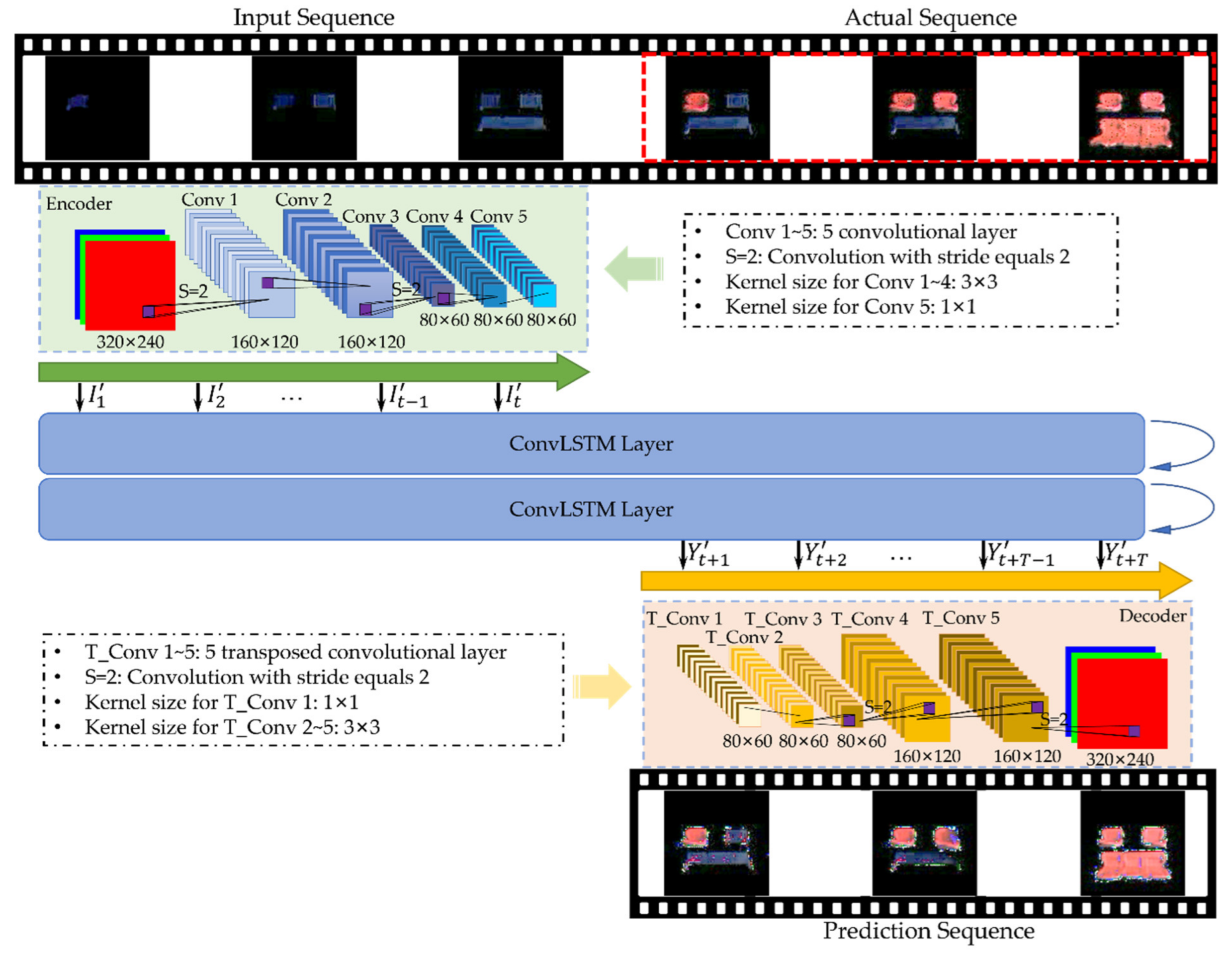
As shown in
Figure 1, there are three main parts in the entire framework. A convolutional encoder processes the input video data and extracts the meaningful spatial features sequentially from a fixed-length video clip. Each frame goes through a five-layer encoder for the purpose of preventing the raw video data from feeding directly into the ConvLSTM layer. By using this method, the encoder will decrease the dimensions of inputs and extract the hidden representations to ease the impact of the data for the ConvLSTM cells.
In order to decrease the dimension of feature maps and retain more information to reconstruct the frame, the stride is set to 2 instead of using pooling layers [
51] when we need to shrink the output dimension. When the stride equals 2, this means the filter slides two pixels at a time. However, the pooling process may erase important details and damage the reconstruction. The spatial output of the first part is a tensor in the shape of 80 × 60 × 32.
This output flows into the second part, which contains the ConvLSTM cells. We use two layers of the ConvLSTM here to retain more spatio-temporal information. This part extends the traditional LSTM to a higher dimension level by changing the input-to-state and state-to-state connections into convolution operations. The spatio-temporal information can be processed through this structure since the spatial information can be analyzed at each time step. Moreover, this part consists of two phases: the learning phase and the prediction phase. The cell state and hidden state of the learning part are initialized with zero, which means there is no history information at the beginning of the training process. After all the input sequence has been fed into the learning phase, the cell and hidden states are tuned accordingly to represent relevant spatio-temporal information. Then, the last states of the learning phase are copied into the predicted phase as its initial states. By doing this, the information of the learning phase is transferred into the following prediction phase.
The recurrent prediction phase projects each future frame step by step, by feeding the states of each ConvLSTM cell directly into the next cell, allowing each sequential cell to sense both spatial and temporal changes. The generated output will guide the frame predictions completely.
Since the whole network structure follows the encoder–decoder network [
52], the convolutional decoder should be the third part. At the second part, the ConvLSTM structure maintains the identical dimensionality of the input and output. Therefore, the convolutional decoder works as the encoder, but in a revised order. Because we need to reconstruct the predicted task sequences, the stride tricks are applied again when we expect bigger spatial output. The spatial output of this part is a tensor with the shape of an input, which means this part uses the transposed convolutional method to map the extracted vectors into the RGB space. The configuration of the encoder and decoder is similar, but their corresponding layer parameters are not shared. This is due to the fact that the encoder and decoder are standing at different time sequences. From the perspective of time, the decoder will always be ahead of the encoder.
This model is an end-to-end training model, as the prediction frame sequences can be generated based on the input frame sequence. Furthermore, there is no need to label the videos since the input sequences and the sequences of actual human actions are already settled down in the dataset. The loss function is calculated based on the difference between the sequences of actual human actions and the prediction frame sequences.
In the following detection section of human faults, the robot will act as a sensitive monitor of the whole workspace and will be equipped with the proposed model. This embedded model makes it possible for the robot to detect potential human faults during the assembly process. Once any human faults are detected, the robot will instantly throw out a warning message, making the human notice and modify it before deterioration. More roles will be attached to the robot based on the prediction and detection results in future work.
2.2. The Assembly Tasks: Learning from Human Demonstrations
Before predicting future human actions, the analysis of human actions and action sequences should be performed first. By watching demonstrations of a human, the system will abstract the spatio-temporal information and transfer them into the prediction model. A human’s advanced perception capabilities will make a big difference when they learn the assembly tasks from other operators. Recently, machine learning technology has been able to mimic this ability, especially through the deep neural network.
Assuming that a human demonstrates an assembly procedure to a robot, the robot will receive a video with the size of . stands for the height and width dimensions of the frame. means the overlapped channels of each frame. denotes the frame number of the demonstration video. Hence, at every time step, a tensor will be collected by the robot, where R denotes the domain of the input space. Given that the tensor I is consecutively sampled by the robot, the demonstration will be represented by a sequence of vectors {I1, I2, … It, … IL}. Assembly tasks learning from human demonstration can be interpreted to extract the spatial information and abstract the assembly strategies of the input video, then process them into the spatio-temporal features.
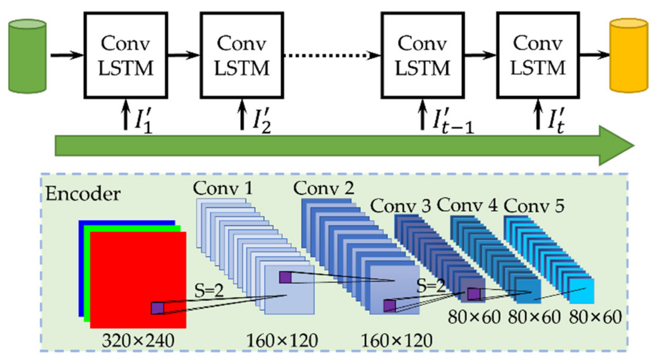
As shown in
Figure 2, a convolutional encoder was used to improve the generalization capabilities of the network. In order to learn how to extract the variety of patterns that construct the input frame, every layer contains multiple filters.
The encoder process is a series of convolutional layers, while the convolution process between the kernels and the input images can be formulated as Equation (1):
where
is the input frame sequence,
is a set of convolutional filters,
is the corresponding bias, and
is the non-linear activation function. At the same time, the conventional encoder will decrease the height and width of the input frame, which will be much more efficient than the raw image input. Here,
is the encoding feature map of input
, but with a low dimensional state. The feature maps
will be passed to the ConvLSTM cells, which can process these spatial sequences and maintain their temporal connection.
After each frame of human operations was extracted by the convolutional encoder, the resulting tensor feeds into an RNN with the same sequence as the raw input video. The ConvLSTM cells are used to obtain the spatial structure and the sequential correlation of the multi-dimensional input vector .
We use RNN here because they are networks with many loops in their block [
53], and this structure can preserve historical information selectively. It is a major shortcoming for traditional neural networks, especially when we need to use previous events to infer later tasks. LSTM is a special type of RNN, and LSTM can alleviate the long-term dependency [
54] problem, which prevents the RNN from being used in long-term predictions. The cell state with several gates works together to control the information going through the cell and modify it optionally by remembering and forgetting. This characteristic makes it practically possible for the LSTM network to trace temporal information for a long time [
55].
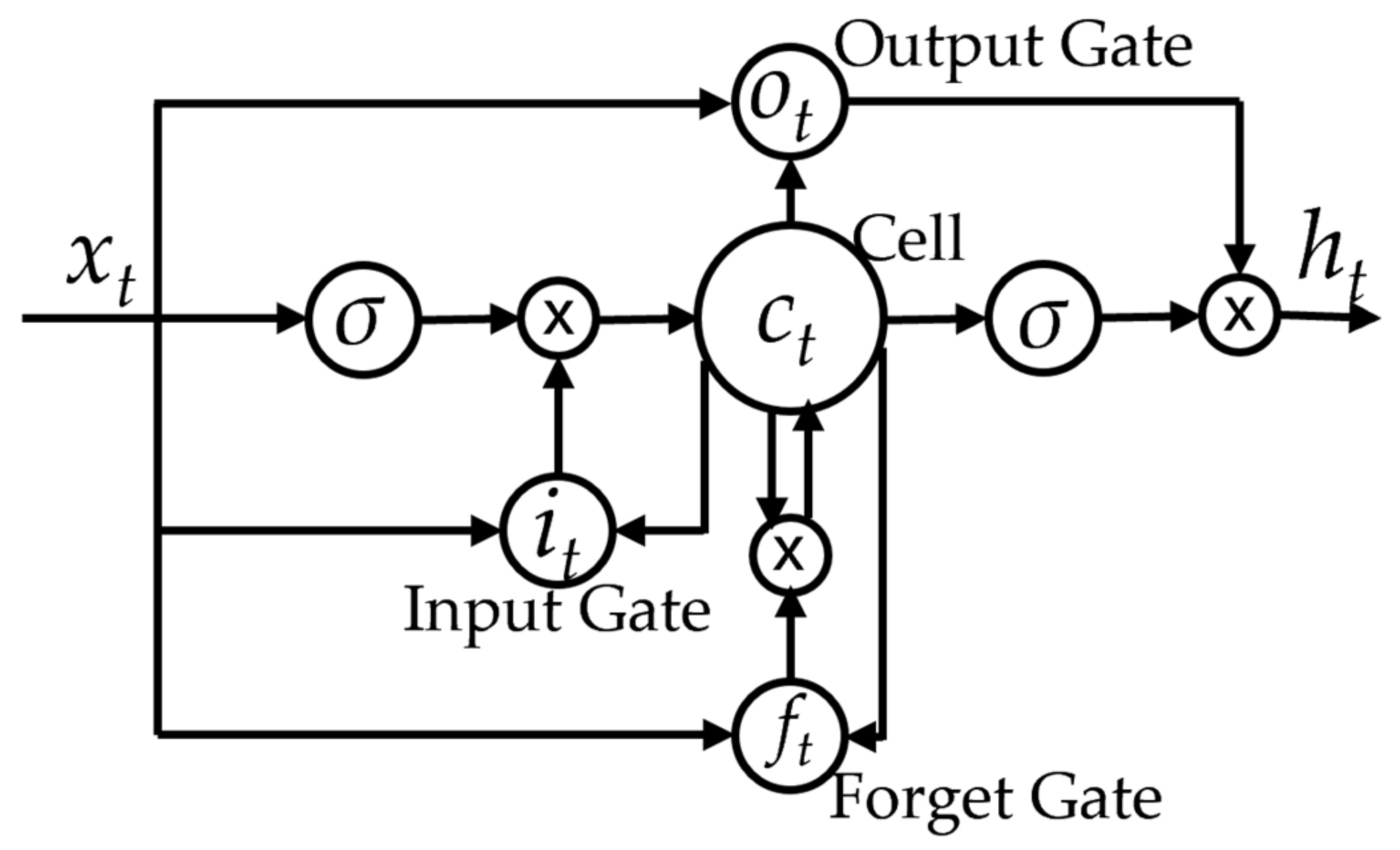
Figure 3 shows the traditional LSTM cell’s structure [
56]. From this figure, we can obtain an idea of how the temporal information flows through the LSTM cell. However, this LSTM cell is not designed for processing spatial correlations, which means this cell cannot be used directly in the spatio-temporal prediction situation. This limitation is caused by the single-dimensional operators in the LSTM cell, both in input-to-hidden and hidden-to-hidden connections. Shi [
49] introduced the 3D operators to the internal process of the traditional LSTM cells and proposed a strengthened variant of LSTM. Therefore, the spatial information along with the temporal information can flow through the LSTM cells easily. They modified the hidden-to-hidden and input-to-hidden operations to a convolutional process and that is why it is named ConvLSTM. The essential equations of ConvLSTM can be formulated as Equation (2):
where
is the input for this block and is equal to the
from the convolutional encoder.
,
, and
stand for the input gate, forget gate, and output gate, respectively.
and
stand for the weights and bias between the input and the gates, respectively.
and
denote the cell and hidden state, respectively.
is the convolution operator and
is the Hadamard product.
As shown in
Figure 4, if we unroll the loop of the ConvLSTM cell, we can understand this process more intuitively. During the learning process of the assembly task, the input video will be processed by the convolutional encoder frame by frame, then the processed output will be fed into the unrolled ConvLSTM cells with the unchanged sequences. Then, the ConvLSTM cells will learn the essential spatio-temporal information and keep it for future use. In
Figure 4, the orange cylinder denotes the tuned model. The orange cylinder is not actually there; we just use this to simplify the pipeline. We also use multiple layers of ConvLSTM cells in our model, although only one layer is shown here. The trained model exists in the whole network structure, as do all the tuned parameters.
It should be noted that the hidden states’ outputs and cell states are both transferred to their sequence cells. All the representations then flow to the following part of the prediction of human actions. Then, the model will reconstruct potential future frames based on its own established knowledge.
2.3. The Prediction of Human Actions in the Assembly Task
The prediction of human actions should be a sequence of frames
, and the prediction process is an analysis of the history of human actions from the input sequences. The conditional probability of the output prediction can be estimated given a human action sequence as in Equation (3):
Then, the prediction of human actions can be realized by the estimation of the output sequences. We can project all the relevant input information to a higher dimensional representation
, and decode this information to its spatio-temporal target output with a decoder. The higher-dimensional representation is extracted from the last part. Hence, the probability can be formulated as Equation (4):
The prediction of future human actions can be obtained from the decoder by choosing the most likely situations, as in Equation (5):
At this stage, the prediction of human actions can be generated according to the information from the input sequences. For the input sequence by human operations, the frame at every time is an RGB image, then the prediction will include spatial and temporal features. However, the prediction will be a rough version due to some trivial information loss during this process.
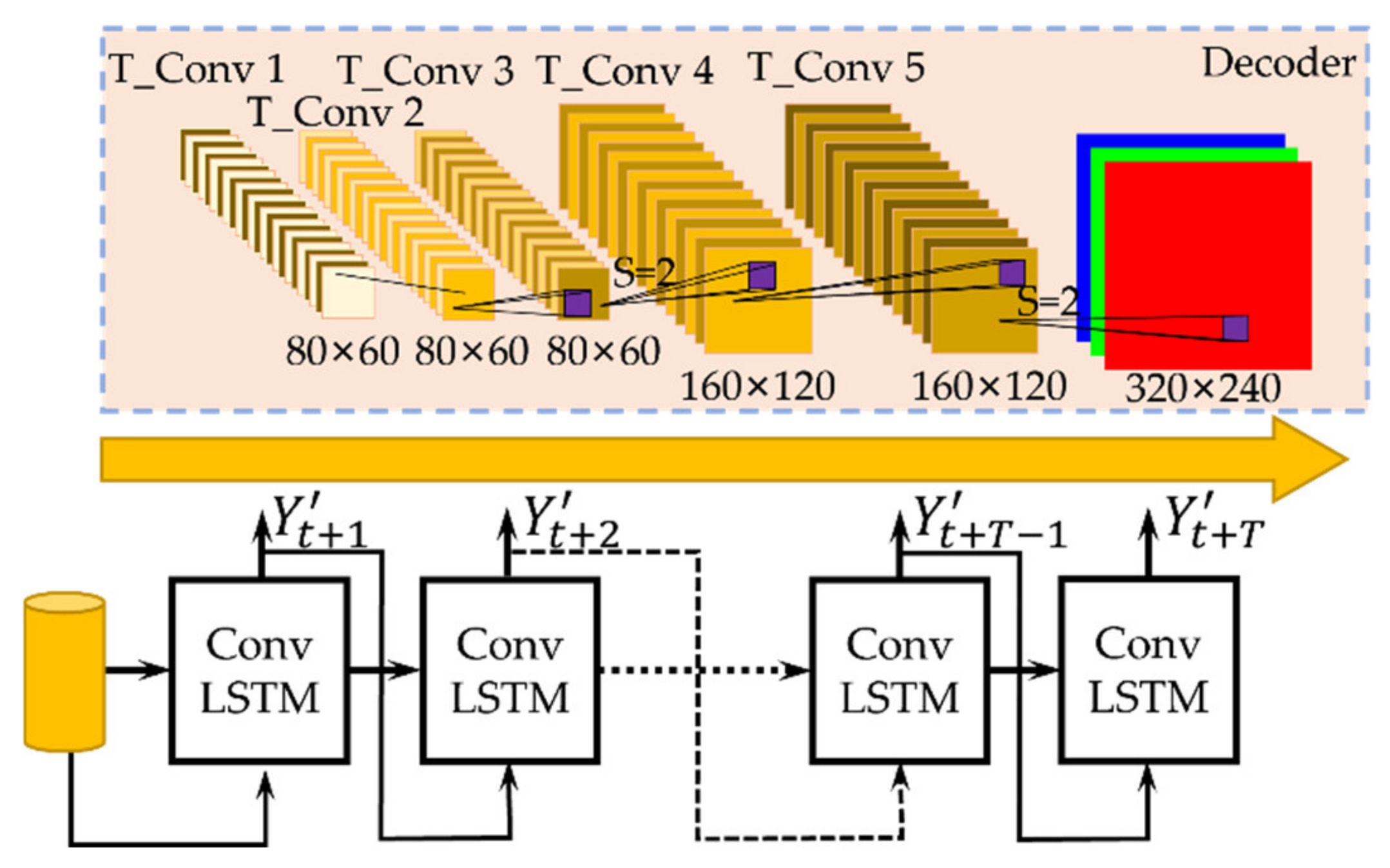
As shown in
Figure 5, the recurrent predictor network infers future actions based on the former ConvLSTM’s cell state and hidden state. The ConvLSTM network will transfer the major features from time
to time
, then the following decoder will make the most of this spatio-temporal information and reconstruct the future frame step by step. From
Figure 5, we can find out that the ConvLSTM infers the representations of the next frame’s features based on previously generated frames. The cell and hidden states represent the future human actions in the feature space, in the shape of
in this case.
Since our goal is to reconstruct the future
from the produced feature maps
, we need a decoder that can handle this process. As is shown in
Figure 6, the convolutional decoder is a fully convolutional network; therefore, the decoding operation is a convolutional process as well. This decoder has a similar configuration as the encoder we mentioned before. It performs the same convolutional operations as the encoder but in a reverse manner. This reverse convolution we used here is the transposed convolution. Therefore, the outputs will have the same dimension as the input sequences.
The loss function is a critical part of the whole framework since the loss function reflects how well the framework models the dataset. When being trained, the model will be optimized, and its parameters will be adjusted gradually until the whole model converges. The loss function will measure the absolute difference between the prediction and the actual action sequences, and it should be well chosen. There are several methods [
57] within this selection. Here, we use the mean squared error (MSE) method as the loss function to train the model using Equation (6):
where
indicates the predicted human action sequences from the proposed model and
denotes the actual human action sequences from the demonstration. The parameters are omitted for the benefit of simplicity.
2.4. The Human Fault Detection
During the assembly or maintenance procedure, the human workers may make some mistakes, which will damage the quality of the product. It is very hard to assign labels to these mistakes under this type of situation, especially in routine videos. This is mostly because the mistakes are often uncommon, or the mistakes present a lot of forms. However, by our method, we can predict the future action sequences based on previous actions, and then after the future outputs are obtained, we can obtain the ‘reference’ for the detection of human faults. Given a set of the test action sequences, this model can compare the similarity of predicted human actions and actual human actions, as shown in
Figure 7. In this way, the model will judge whether this action is a fault.
When inspecting the next actions, human faults will be more likely to be noticed, as the trained model may reconstruct a different action sequence. In order to assess this detection quantitatively, the reconstruction and practical actions will be generated and compared in an assessment method.
In this model, we did not only use the MSE method, because MSE may cause a lot of noise. The rough prediction is not exactly equal to the practical sequences, and this noise will be exaggerated by MSE. The differences are not fixed at the pixel level. Hence, another main assessment parameter we used here is the structural similarity (SSIM) [
58,
59] method, which can be defined as Equation (7):
where
,
,
,
, and
denote the mean of
, the mean of
, the variance of
, the variance of
, and the covariance between
and
, respectively.
and
are two small positive variables to stabilize the division when the denominator is close to zero. SSIM is a method for measuring the similarity between two images.
Meanwhile, we use a score function to distinguish the fault actions. Since there may be a different measurement in every scenario, we need to project the score from zero to one. The score function [
60] can be defined as Equation (8):
where
denotes the parameter list, and
and
denote the minimum and maximum values of the parameter list, respectively. With Equation (8), each datum will be scaled from 0 to 1 internally. In this case, we treat the clips as a series of images. Thus, every video clip has two parameter lists, the MSE and SSIM lists, which should be calculated frame by frame. Since we need to compare two video clips, the frame-by-frame comparison we used here can be described as Equation (9):
This algorithm will calculate the essential difference during our tasks because the pixels in videos are highly organized in both spatial and temporal space. It can evaluate the output features using a rescaled composite approach and provide a robust way to process the dynamic data. The local spatio-temporal activities can be compared in a very efficient way.
Practical task sequences will have a very high similarity since they are roughly the same as the sequences used to train the model, while sequences that include human faults will have low similarity. Two situations may occur during this detection process. First, routine task sequences keep feeding into the model, and suddenly a fault happens. In this case, the predictions will be generated based on the routine task sequences, and the similarity between the prediction and the next practical sequences will be decreased. Second, the fault already went into the model and generated new predictions. In this case, however, our method also works. The faulty tasks will cause the prediction reconstructions to form a strange pattern compared to the normal task sequences, since the model has no relevant information to predict the future fault sequences. This unseen data seem to be more difficult to reconstruct due to errors evolving both in spatial and temporal space. Generally, we would follow the first situation.
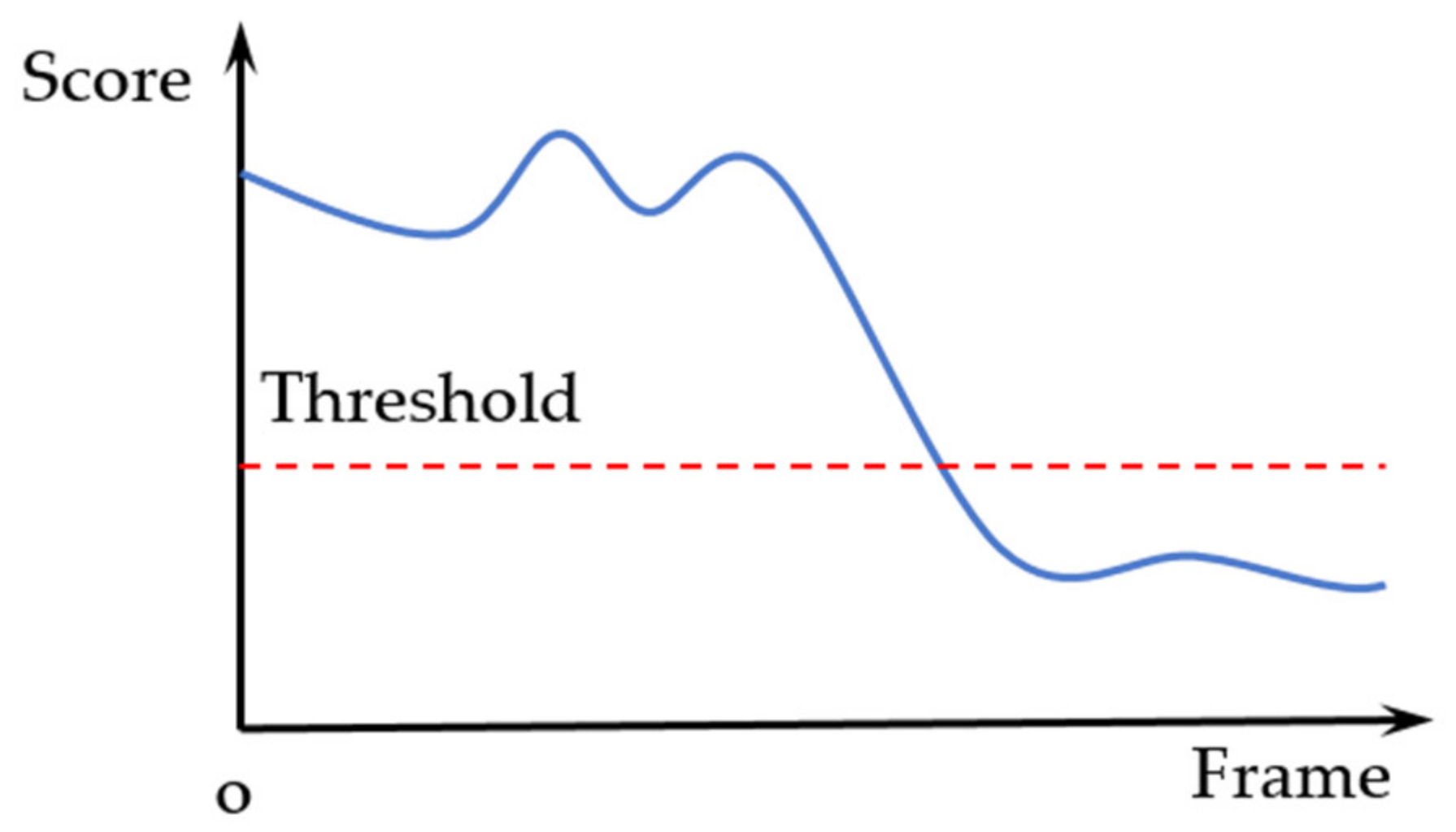
Keeping the similarity above a certain threshold can be used to detect the human fault during the assembly or maintenance tasks, such as in
Figure 8. If the score value is lower than the threshold, we assume that the model detects a fault action.
3. Results and Analysis
3.1. Experimental Setup
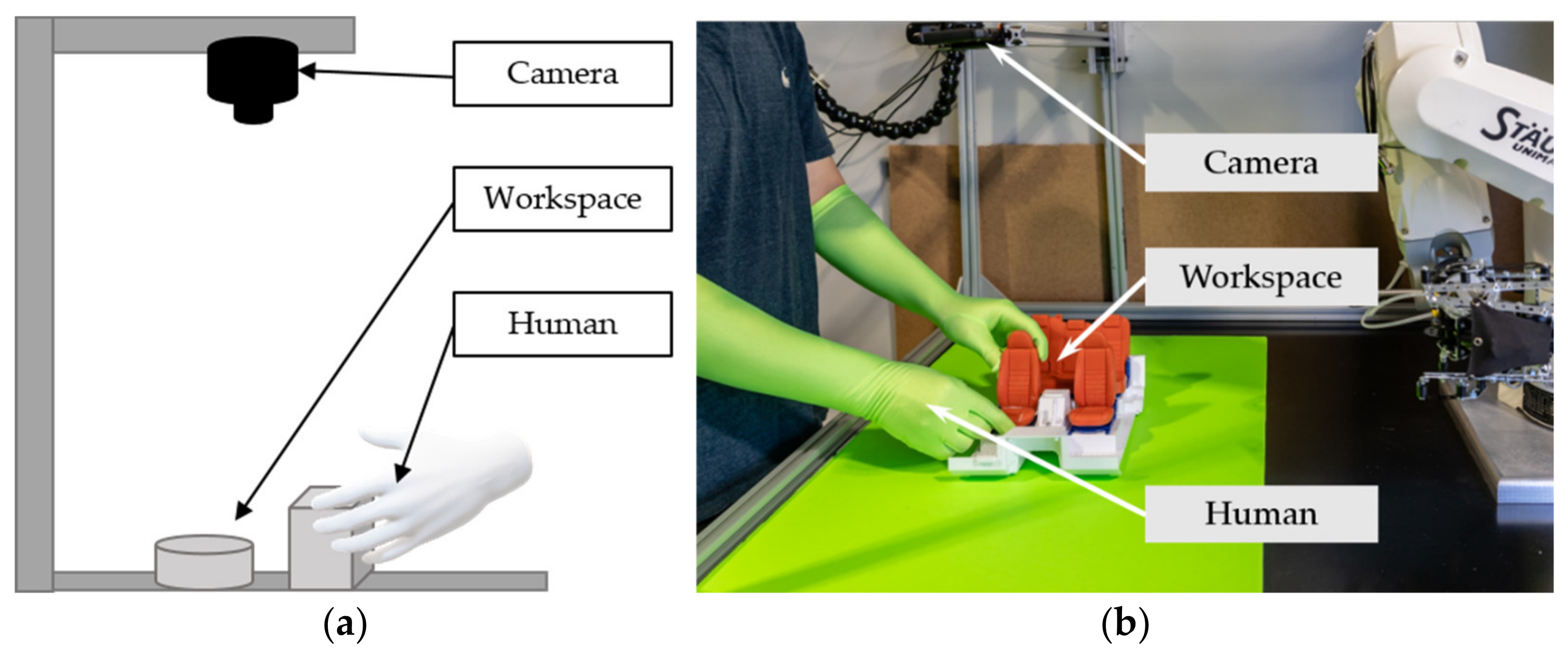
We describe the physical setup for our dataset collection and the subsequent experiments in
Figure 9. The camera is mounted overhead on the top of the workspace and provides an overview of the changes in the human actions in the workspace. The distance from the camera to the surface is approximately 0.6 m. The camera’s resolution is 1920 × 1080 pixels, and the frame frequency is 30 Hz.
Figure 9b shows the real setup of our project, and the robot stands right in the workspace. During the experiment, the lighting conditions should be as consistent as possible to prevent introducing unexpected shadows. The experimental setup in
Figure 9 can provide a reliable platform for data acquisition, and the configuration can easily adapt to the real robots, which would be suitable for the detection of human faults and future projects.
The experiments were deployed based on the TensorFlow 2.5.0 framework in the Python 3.8 environment. The NumPy version was 1.19.5 (Travis Oliphant, Provo, UT, USA); the pandas version was 1.3.0 (Wes McKinney, Greenwich, CT, USA) and the OpenCV version was 4.5.3.56 (Intel Corporation, Santa Clara, CA, USA). During the training phase, the Adam optimizer was adopted to train our proposed model. The learning rate was first set to 0.001, and the learning rate decay was applied to improve both optimization and generalization. The weight decay was used to avoid overfitting as well. The model was trained on 2 GTX-1080 GPUs, and the training process stopped when the early stop epochs were achieved without performance improvement or when the maximum iterations were completed. All the network hyperparameters were updated iteratively and selectively saved based on the validation process. During the testing phase, each video was preprocessed into the same dimensions as the training samples to calculate the scores to detect the potential defects. The area under the precision–recall curve (AUPRC) was applied as the measurement metric to choose the threshold. In this study, our model was used to detect the human faults in the assembly scenario and to eliminate complex predefined processes.
3.2. The Dataset
Recently, there have been a lot of public video datasets available. However, these datasets focus on different situations and are too complicated for our purpose. Generally, the samples from these datasets do not contain essential information to describe the industrial assembly process. During the assembly process, the industrial environment is very different from normal life scenarios. For instance, commonly, the background of the environment is more stable, and most of the sequences of actions are repetitive. Since the public datasets we mentioned before belong to other domains, they may not carry enough representations for industrial assembly or maintenance applications. Therefore, we have to build a specific dataset [
61] suitable for industrial purposes, and it should be compatible with the prediction of human actions and experiments on the detection of human faults. To build an industry-wise dataset to simulate the industrial environment and to verify our model, the actions should be ordered, and the background should be flux-free. The samples collected from this workspace should be similar to real industrial contexts. Then, we will apply our model to the dataset to mimic the applications in a real industrial scenario.
The dataset contains two classes of videos, the normal videos and the fault videos. The normal videos are used to train the model and validate the prediction, while the fault videos are used for the detection of human faults. There are two types of sequences in the normal videos. The videos of different sequences can verify the prediction ability of the customized model. Meanwhile, there are three types of faults in the fault videos, such as unfixed parts, exchanged sequences, and missing parts. First, we recorded 37 normal videos directly from the camera; the size of these raw videos is 1920 × 1080 at 30 fps. These videos needed to be processed. The green background had been removed first, then they were resized; we set the final size to 320 × 240 in 10 fps. After completing the resizing, a 100-width sliding window [
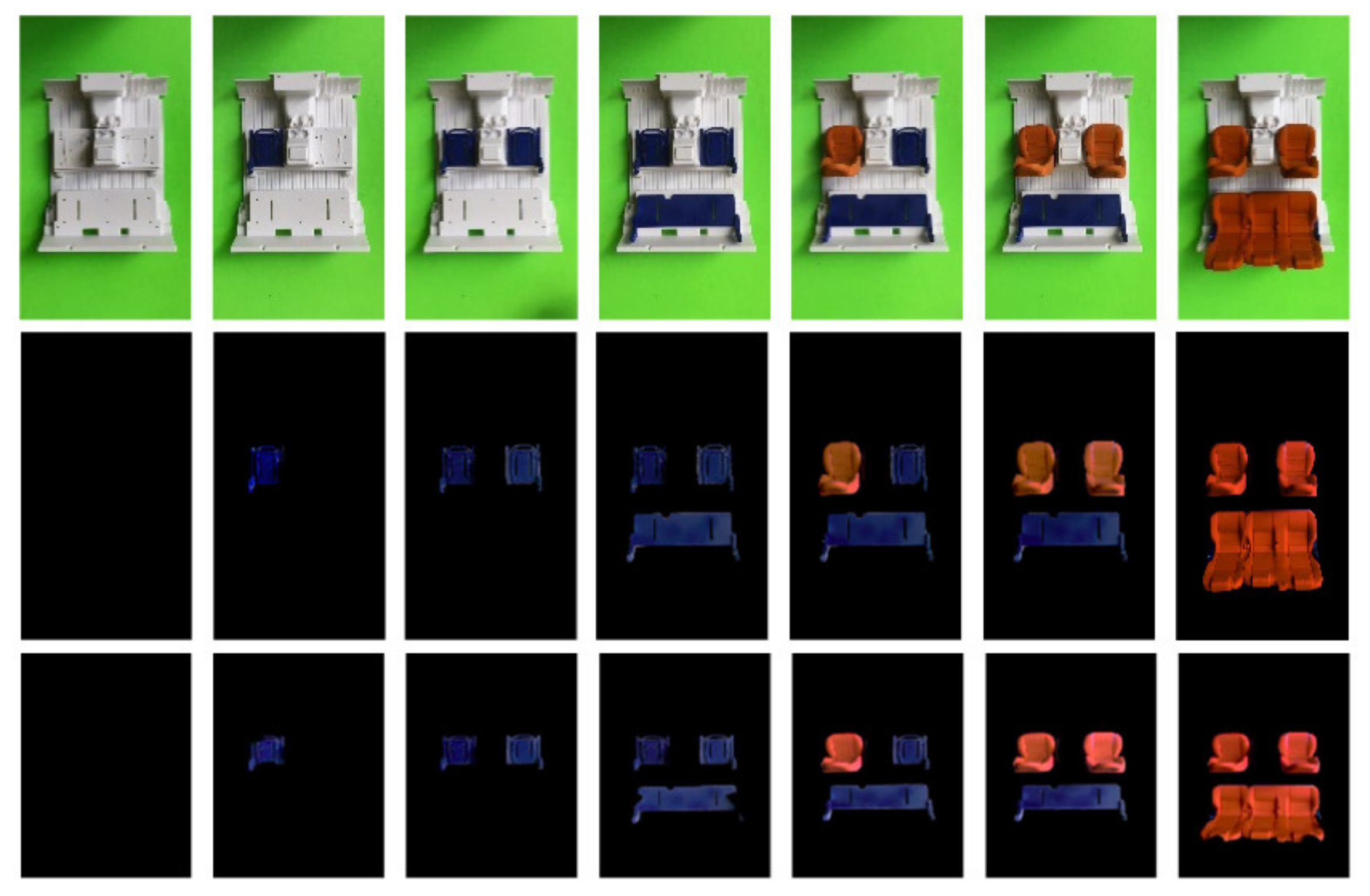
62] was applied, and the stride was set to one frame. The videos were to be cut into clips according to a 100-frame length. Around 4500 clips were obtained after these processes, where each video clip shared the same dimension: 100 × 320 × 240 × 3. The last dimension, dimension 3, means we used all RGB channels on our model. There is no label in this dataset, and it only contains video clips with actions from the assembly process. We show one example from our dataset in
Figure 10. It can be seen from
Figure 10 that the first row denotes the original videos, with a resolution of 1920 × 1080, and the second row denotes the background-removed videos, with a resolution of 1920 × 1080. However, the image is still too big for the computation, so we used the resized videos in the third row, with a resolution of 320 × 240.
The length of each video clip is 100 frames, and we chose 50 frames as the prediction span. The selection of this time span is explained in the next section. This time span ensures that the model can cover enough motions and process them into meaningful information while maintaining efficient calculation. For humans, even if each clip is different, they can learn from long-term video clips and obtain useful spatio-temporal information. The challenge lies in embedding this functionality into the deep learning model and performing the same tasks. This dataset will be able to verify this and also meet other subsequent challenges.
3.3. The Selection of the Prediction Span
The choice of the prediction span is critical for the following applications: In the training process, we need the specific prediction length to calculate the loss function. The prediction span should keep the expressive assembly information and restrain the calculation resources. Meanwhile, as for the prediction and detection process, we need the proper time span to generate a clear output.
Considering the size of the dataset and the parameter settings, the model can afford to make the feature number relatively small. Here, we chose the kernel size of ConvLSTM as 3 × 3 and the feature number as 32. During the training process, we tried to enlarge the model, then tuned the parameters accordingly. This led to the many differences in the hyperparameter settings, and the model with the best validation performance can be adopted to future applications.
All the data will be shuffled during the training process, and it will make it possible for the model to gather sufficient temporal information and to improve its performance. The optimizer in our model is Adam, which can converge in a fast way. As for the learning rate, we used the exponential decay method to reduce the learning steps over time. Small improvements in the loss function can make a big impact on the performance of the model. The early stopping method was applied to stop training when the performance stopped improving for multiple epochs.
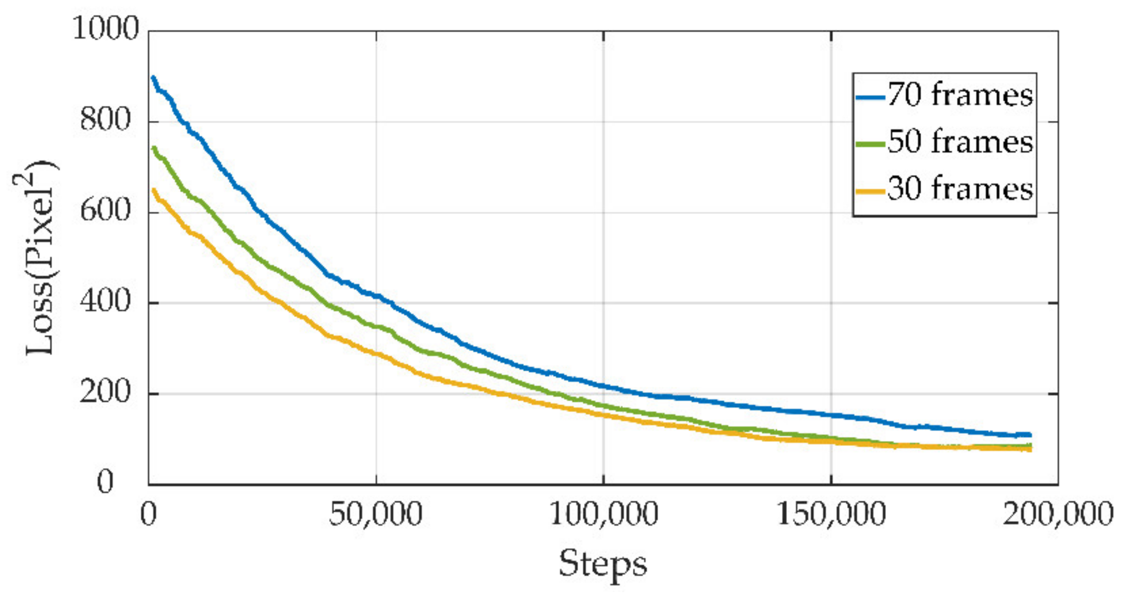
Figure 11 shows the result of our loss comparison in different prediction spans. We compared three configurations to show the influence of the prediction span. As is shown in
Figure 11, the loss function needs a longer time to converge with a bigger prediction length. The model with a prediction length of 70 frames is very hard to train because the model tries to regenerate the information of the following 7 s. Moreover, the output is not sharp, especially at the end of each prediction clip. On the other hand, the model with a prediction span of 30 frames converges relatively easily and its initial loss is smaller than the other models. Compared to other models, it takes the shortest time in the training process and the output prediction clips are sharper. However, the output is not long enough to cover the action sequence, which may render the subsequent fault detection uncooperative.
The model with a span of 50 frames is a better trade-off in this project. It can converge in an efficient way and achieve a similar output quality as the model with a span of 30 frames. Moreover, the 5 s span can cover most of the human actions. This coverage can ease the difficulties in fault detection. Taking the calculation resource into account, the model with a prediction span of 50 frames was chosen for the following applications.
3.4. Prediction of the Assembly Task
The trained model can predict human actions according to the input video clips. The output of the model is intuitive since the output shares the same dimension as the input video clips. We concatenate the prediction after the input to show the performance of the model.
The output video from our model needs to be unrolled into the image series to analyze the results.
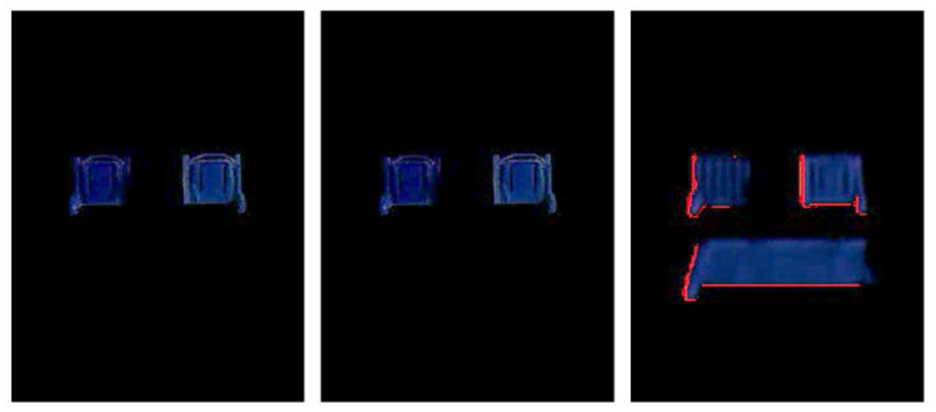
Figure 12 shows the results of the prediction of the seat holder. The first and second images are from the input video clips, and the third image is from the output prediction.
Figure 12 indicates that the prediction of our model is correct according to the human demonstration, in which the third seat holder is being installed after the installation of the first and second seat holder.
Figure 12 shows that the prediction result presents a good image quality except for being a bit fuzzy, which suggests that our method can extract the fundamental information from the historical demonstrations and reconstruct them in a decent way. To be more specific, some orange lining appears at the edge of the seat holder; these noises may have been introduced during the background removal process. When we remove the background, some unnoticed pixels will be mixed around the intersection of the foreground and background, and it is very difficult for our model to predict these pixels. Although there are some noises occurring in the prediction process, they have no influence on our application since we only need the action sequence and vital spatial information.
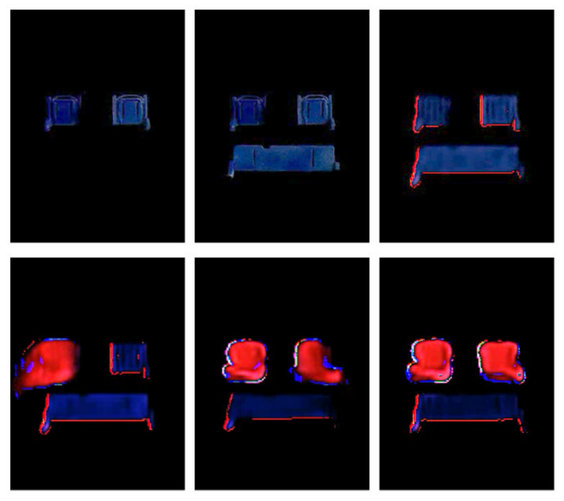
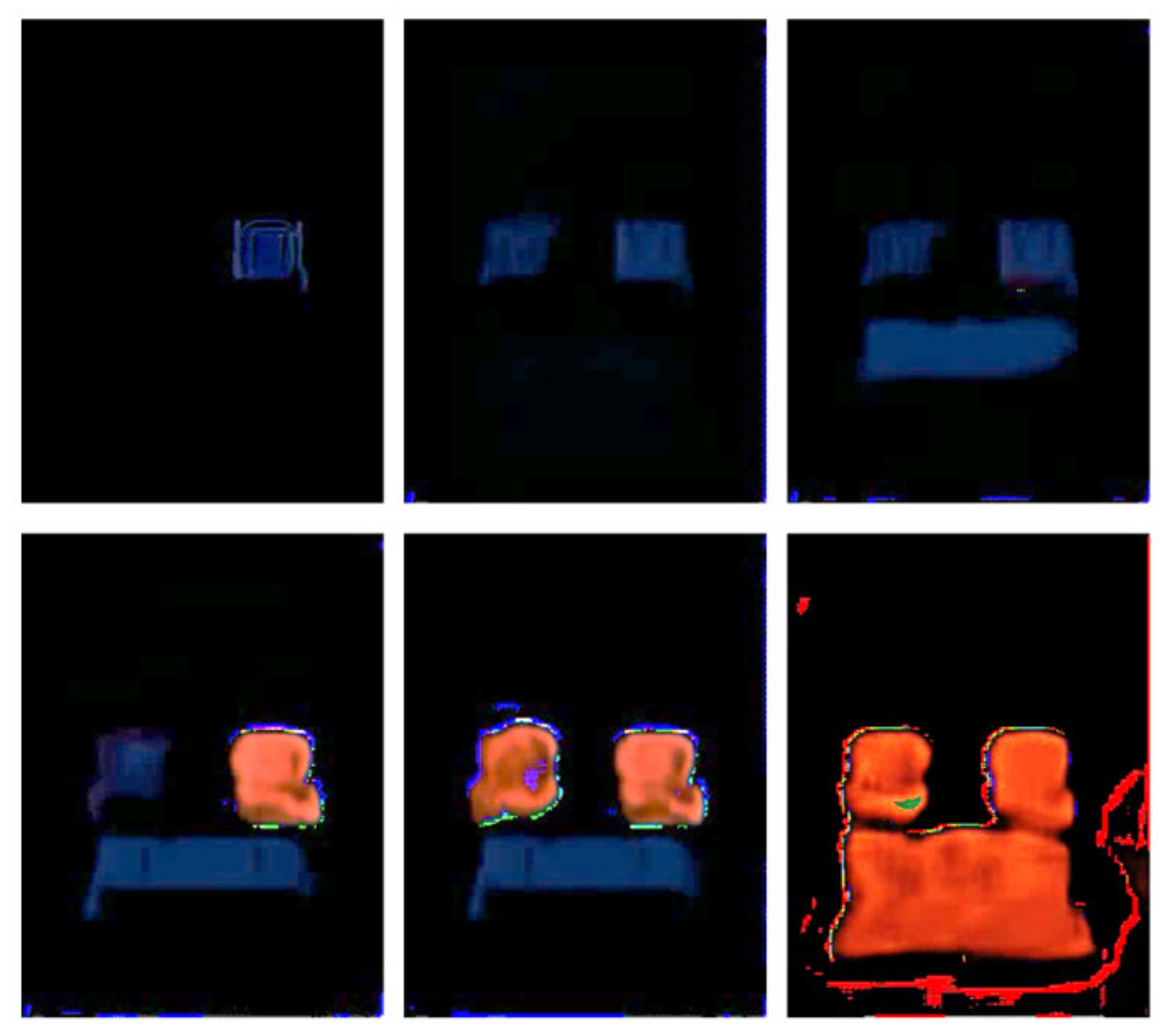
Figure 13 shows the prediction of the succeeding action sequences. The first two images are from the input clips, and the following images represent the prediction of our model. It can be seen that the prediction from our model is matched to the real demonstrations, i.e., installing the left and right seats after the installation of all the holders. The positions of the left seat and right seat are well generated with similar noises. Although the right seat becomes a non-rigid part in the fifth image, the model attempts to predict the motion according to the information of the temporal pixel.
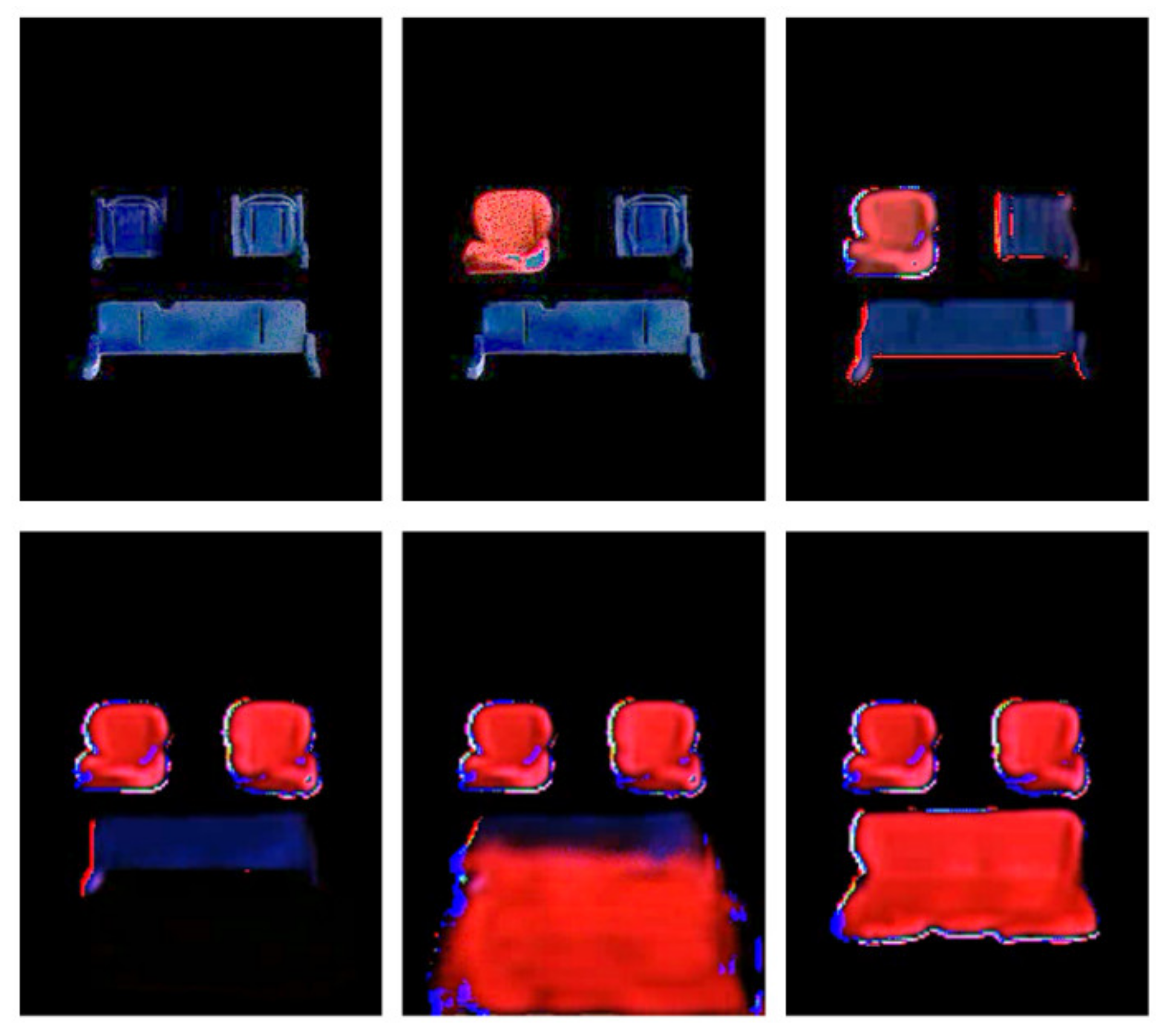
Figure 14 shows the output from our model of the installation of the second and third seat. The model needs to rebuild the future process based on its knowledge. The first two images are from the input sequence, while the rest of the images are from the subsequent prediction generated by our model. Although the construction of future actions contains some noises and some specific parts transform into non-rigid objects, the model can predict future human actions appropriately in this case as well.
Our model can deal with a lot of industrial processes if sufficient human demonstrations are provided. Here, we use the exchanged assembly sequences to verify it. The same experimental setup and similar model can be adapted, while the dynamic information changed dramatically. The installation of the holders and their corresponding seats were switched to perform these real demonstrations. Then, a dataset was constructed based on these demonstration videos to train the proposed model.
Figure 15 shows the images from the prediction results of the exchanged sequences. The first image is from the demonstrated assembly clips, and the others are from the prediction sequences. We trained the model with a relatively small dataset, which explains the blurry prediction and the increasing noises. New predictions were obtained successfully through the trained model. Meanwhile, the results indicate that the model can predict other industrial procedures with an appropriate dataset.
These predicted situations above indicate that our model can predict multiple frames for human assembly processes. The prediction length is 50 frames, which covers a 5-s time span. Here, the predictions of our model are reliable, but if we extend the prediction to be longer, the model may output more blurry results or even some failed predictions. This is because the input information is too far for the model to reconstruct a useful sequence. Although there are some blurs existing in the prediction sequences, the model can still fetch the core information for video reconstruction. For example, in
Figure 13and
Figure 14, the model can predict the motion of human actions and the desired positions of the parts. In summary, from the perspective of both time and space, the model can learn critical information from the human demonstrations, such as the colors of the parts, the shapes of the parts, and the motions through every sequence. Then, the model can reconstruct the future human actions based on this historical information in terms of the level of space and time. Based on this ability, we will extend this model to the detection of human faults and evaluate it in the following section.
3.5. The Detection of Human Faults
The prediction performance of our model was evaluated in the previous section. Although the model can extract historical information and reconstruct future human actions, we can take more advantage of this ability and use it to detect human workers’ actions and monitor the possible faults within the assembly or maintenance processes. Since the output has the same format as the input clips, we can output them together as well as the main evaluation parameters. Then, we can analyze the detection performance along with the intuitive outputs from our model.
3.5.1. The Faults of the Unfixed Parts
Sometimes there are cases where the assembly parts are not fixed in the industrial scenario. This fault will influence the quality of manufacturing and cause potential risks for the subsequent processes. This fault can be detected with our model in an intuitive way.
Figure 16 shows one of these situations. In
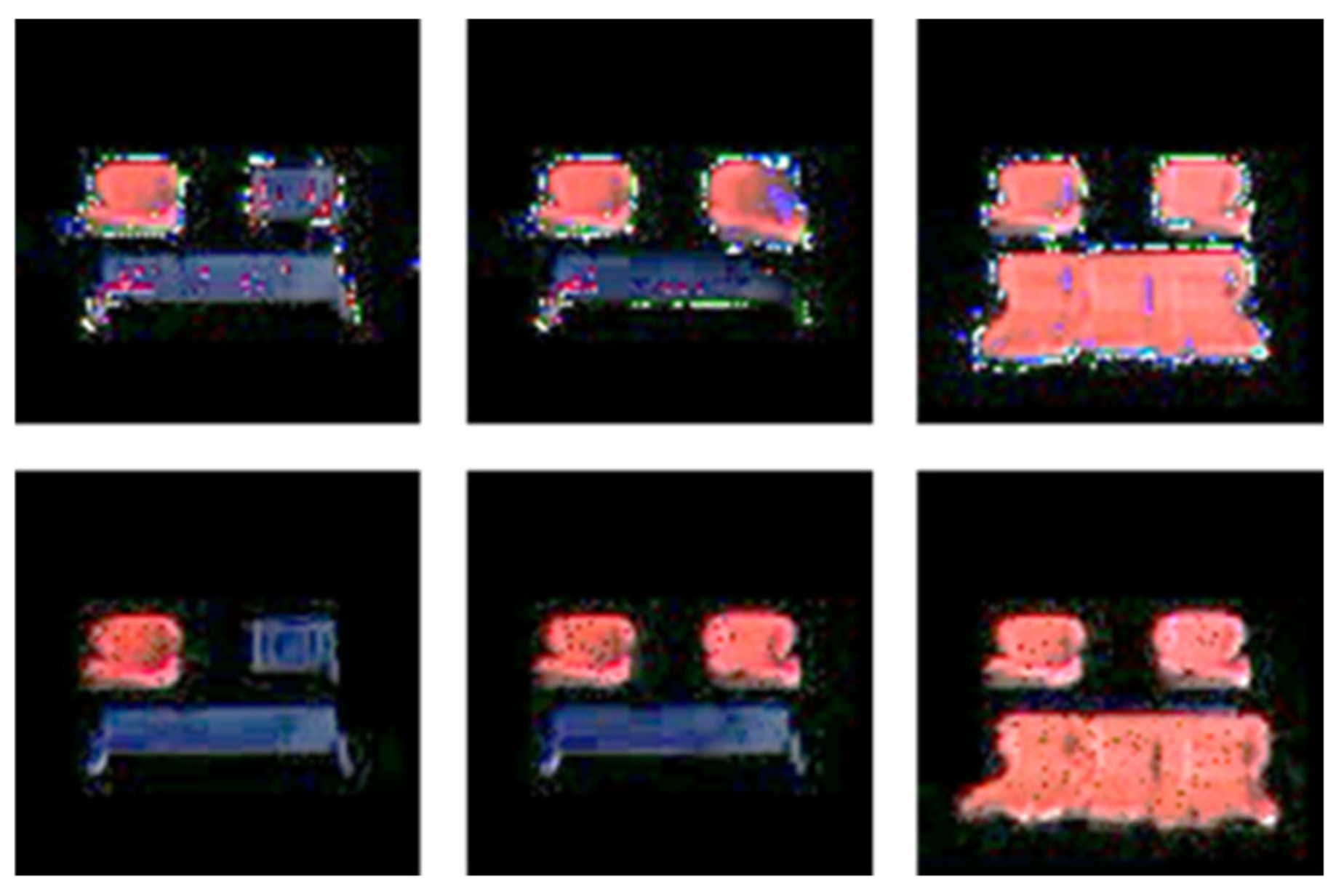
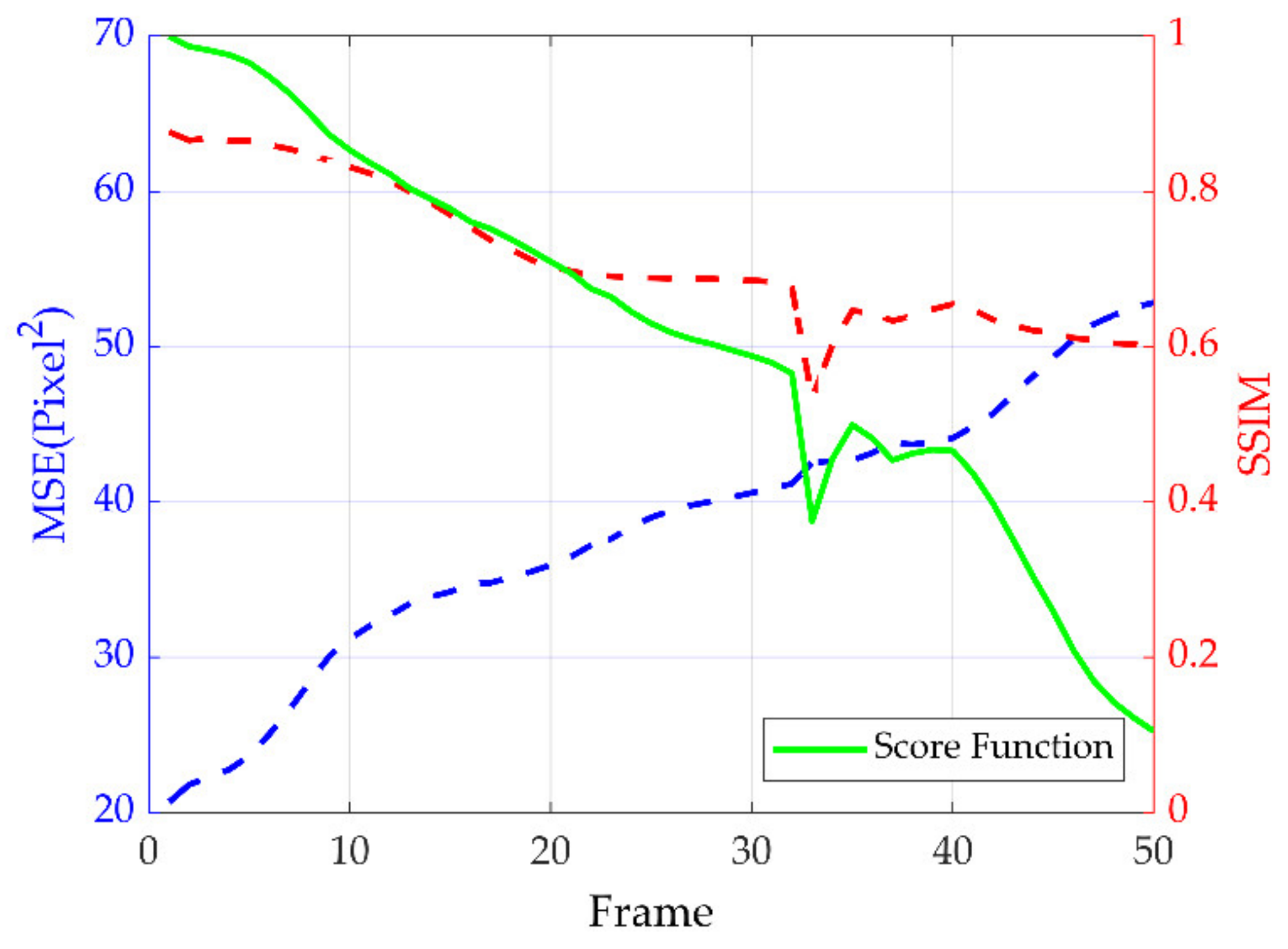
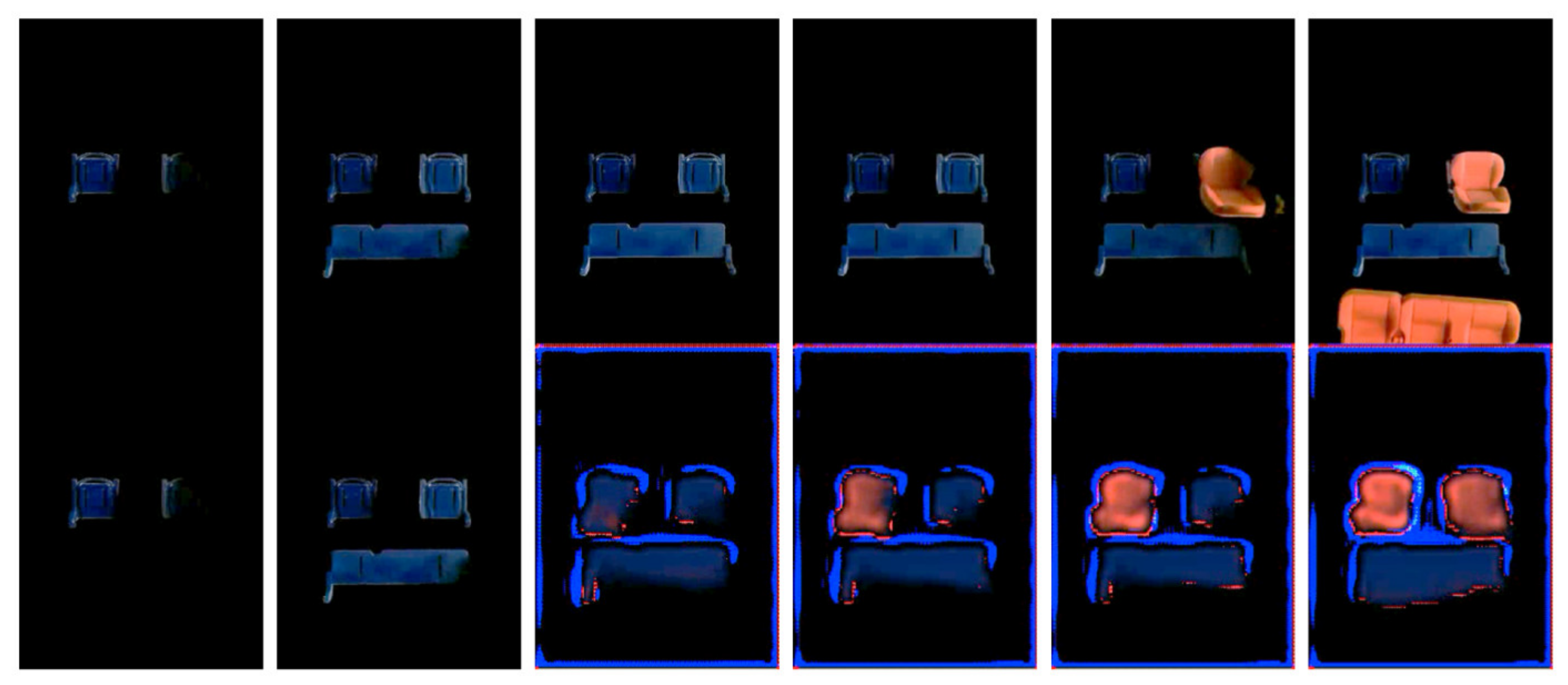
Figure 16, each image has two parts: the upper row stands for the actual test sequences, while the lower row stands for the prediction output based on the knowledge of our model and the input video clips. Moreover, the first two images are from the input clips, so they own identical upper and lower rows. Then, the subsequent images can be used to detect faults. We concatenate the actual test sequences and the prediction of the model output to generate a clear comparison between them. It can be seen that the right seat is not properly fixed in the fifth image and the sixth image, which means that the falling off of this seat is a fault situation. As such, our model cannot predict this situation and the difference between the test sequences and the prediction output is increasing. Before the right seat fell, the prediction matched the test sequences quite well, since all the historical information had already been fed into the model. Then, the model generates the routine actions of installing the back seat, rather than falling off as in the test sequences.
Figure 17 shows the corresponding score function value. The score function drops dramatically when the model detects the unfixed part. The dropping score can be used to locate the specific time step in this process. The gradual decrease in the score indicates that the more differences between the test sequences and the prediction, the easier the human faults can be found in the whole process.
Based on the score function, our model can detect the unfixed parts during the assembly processes. In order to check the accuracy of unfixed detection, we throw a dataset that only contains unfixed part scenarios into the model.
Table 1 shows the detection results; the model can handle this scenario well, with only five cases of detection failure occurring among 120 samples. Hence, the error rate was about 4.2%. Most of the errors arose at the beginning of the unfixed part falling off.
3.5.2. The Faults of the Exchanged Sequence
In the industrial scenario, a worker may install some parts according to undesired sequences by mistake. This fault may cause the assembly process to pause or fail, and it can be detected by the model as well.
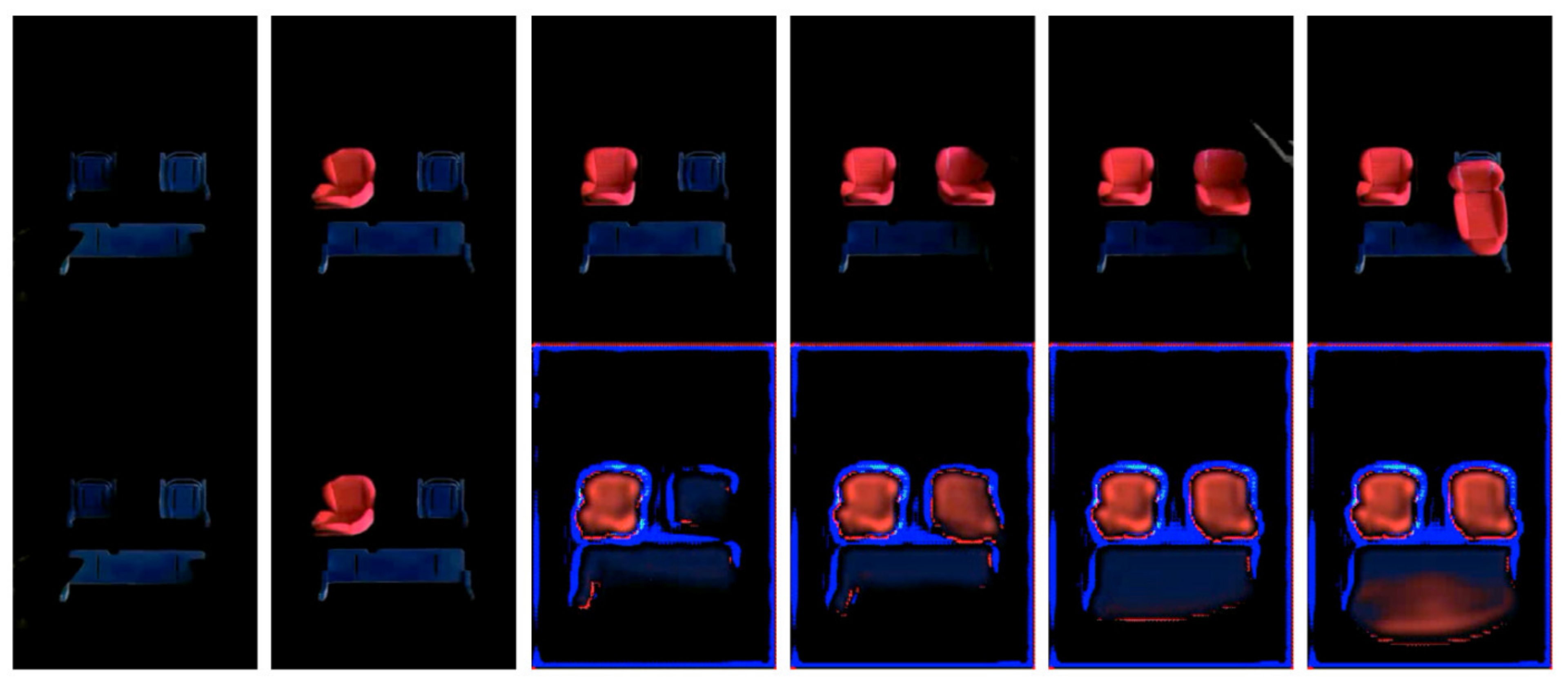
Figure 18 shows one example of an exchanged sequence fault during the test. The configuration is the same as in
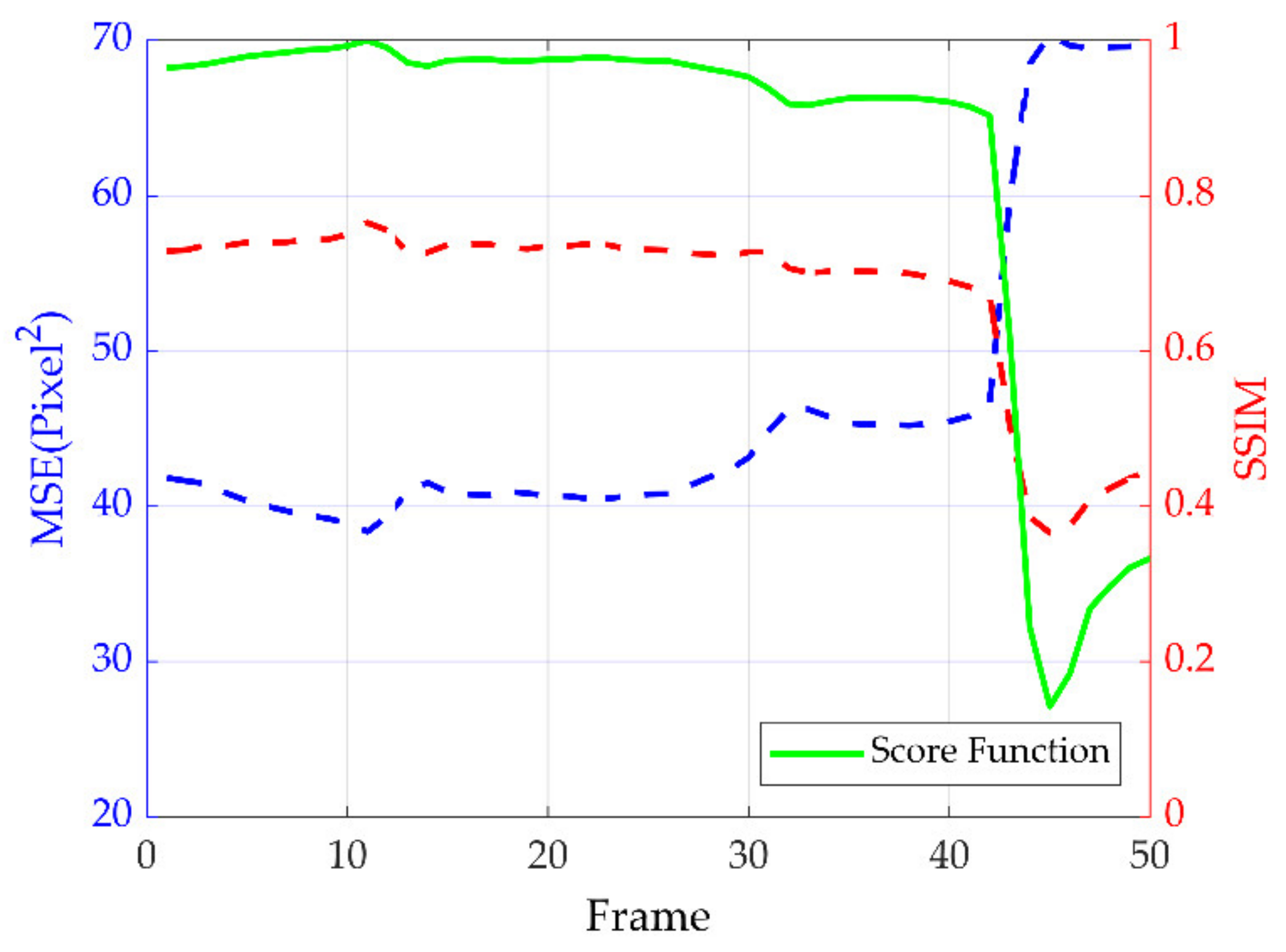
Figure 16. The figures in the upper row show the test sequences, and the figures in the lower row show the output of our model. The first two images are from the input clips and the subsequent images show the comparison of the test sequences and prediction output. In this image group, humans install the right seat holder first, instead of the left seat holder. The model has never seen this scenario before, so it is very difficult to construct the following process. That is why the prediction in the third image of
Figure 18 is the right seat and has also been distorted. Every unseen frame in the input clips deteriorates the following prediction. During this whole process, since the model has only learned to infer human actions, the prediction of the unseen scenario becomes similar to the original training dataset.
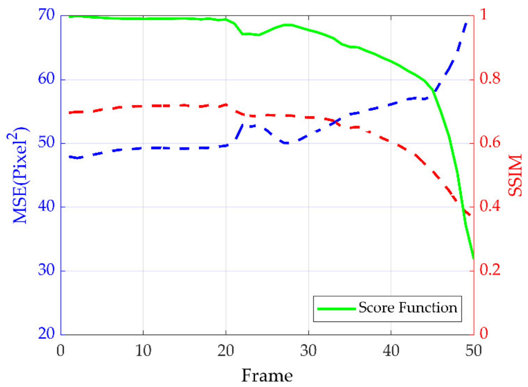
Figure 19 shows the matching score function value of this exchanged sequence. The score function drops gradually at the beginning of the prediction since the input is completely different from the normal training dataset. At the end of this sequence, the low score can be an apparent symbol to raise a detected fault. The trend of this score function matches the differences between the test sequences and the prediction; hence, the bigger difference tends to be faultier for the model.
Exchanged sequence faults are more difficult to detect due to multiple possibilities. For the purpose of checking the accuracy of exchanged sequence faults, different samples containing exchanged sequences were fed into the model. The model will output an unpredictable sequence due to the unseen input information; therefore, the score function will reflect these differences.
Table 2 shows the detection results of the exchanged sequences. There are 18 detection failures within the 330 samples; therefore, the error rate is around 5.5% in this scenario. This result indicates that our model can detect the faults in the exchanged sequence during the assembly process.
3.5.3. The Faults of Missing Parts
A worker may forget to install some parts in the process of real assembly or maintenance. This fault is crucial for some industrial situations, such as when other parts are running based on the previous parts. If this fault occurs, the whole process should be ceased otherwise it will negatively impact the quality of the products. After we feed clips of this situation into our model and track the prediction and the score function, our model can handle this fault in a similar way.
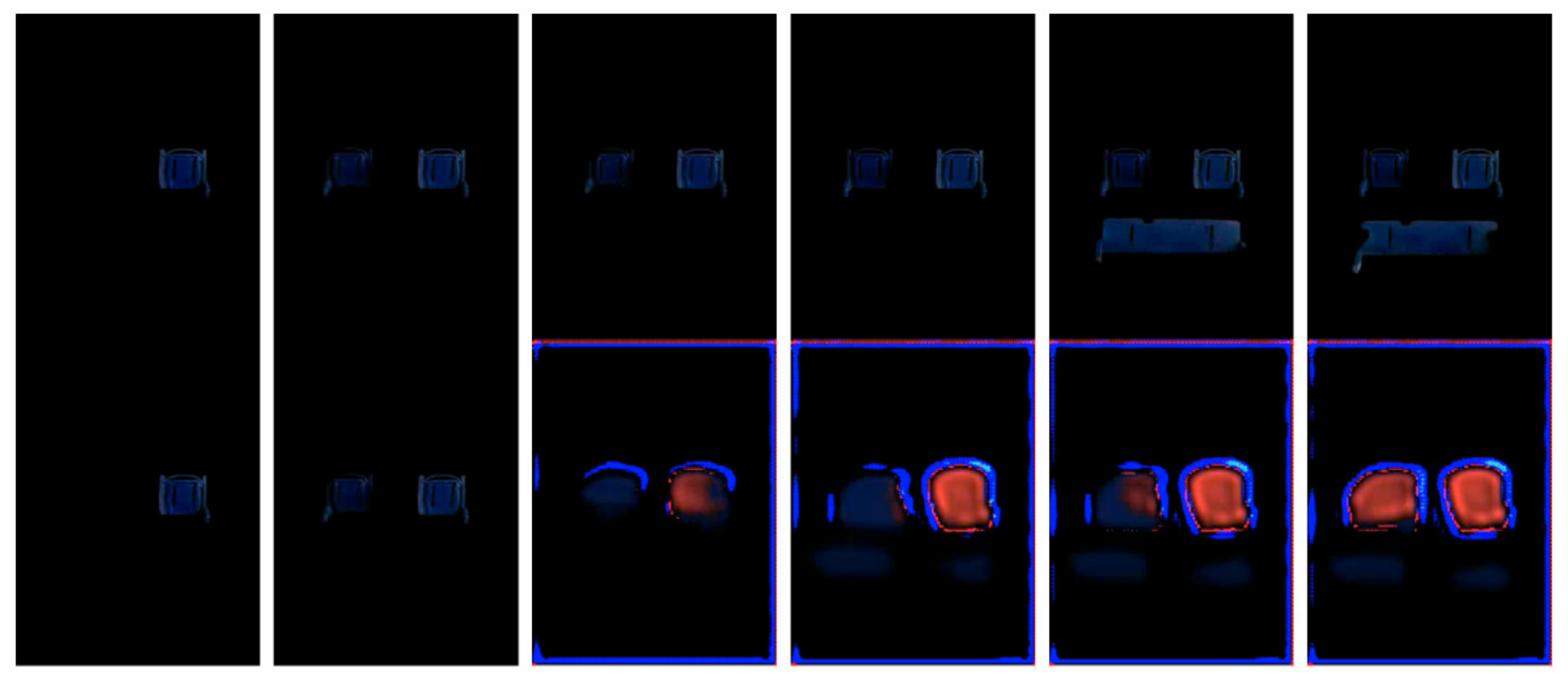
Figure 20 shows one example of a fault of a missing part in the process of evaluation. We use the same layout as the previous scenario. The upper row shows the test video clips, while the lower row shows the prediction process of the missing part. As with before, the first two images are from the input video and the others represent the comparison between the actual sequences and the prediction. The missing left seat in
Figure 20 is not a normal situation; hence, the model cannot predict it correctly. The normal left seat installation is constructed properly by our model, as the information needed was already encoded in our model, which will lead to a big difference in the actual test sequences. The resolution of each part seems to be equal during this prediction process.
Figure 21 shows the corresponding score value of
Figure 20. The gradual decrease in the score results in the model predicting the motions of different parts in the workspace. The lowest point in the score indicates that the fault clips form a clear contrast with the prediction constructed by our model. It should be mentioned that the timestep is changed and does not match well because the missing part changes the length of the whole process.
Sometimes missing part faults and the exchanged sequences can be mixed. For example, we can consider the following part missing at the beginning of the exchanged sequence. The main difference between these two types of faults lies in the final state of the assembly process. The missing part faults are uncompleted at this stage. For the sake of testing the accuracy of the missing part faults, the dataset with these faults was evaluated by our model.
Table 3 shows the detection results for missing parts. The total number of these faulty samples is 250, and there are 13 failures during this evaluation process. Hence, the whole error rate is 5.2% in this scenario. This result reveals that the model is able to catch missing part faults during the assembly process. Most of the failures happen at the beginning of the detection of the missing parts, so these failures may be caused by the uneven spare time in the input clips.
3.6. The Performance of the Detection
We used a laptop with an i7-7700HQ mobile processor and a Nvidia Quadro M1200 GPU to handle the pre-processing and evaluation processing sections. The performance requirements in the processing and evaluation sections do not have high demands. The training section, on the other hand, needs more calculation resources and power. We used a desktop with an i7-6700K processor and two sets of GeForce GTX 1080 GPU to train and validate the model. The training process could last for days; in such a case, the trained model would be stored and ready for evaluation.
As is shown in the last section, the model can detect the actions of human faults based on the prediction of actions. The model evaluated on the other dataset contains both normal assembly actions and human faults. The threshold score is applied to detect the fault actions during the manufacturing procedure. We can consider this as a binary classification problem and apply the confusion matrix [
63] to show the performance of this model.
Table 4 shows the experimental results of our method. There are several false alarms and missing detections in the detective situation of human faults. Moreover, we found that most of the false alarms would happen at the beginning of the detection process and the miss would happen when the transition progressed from the normal actions to the fault actions. This is perhaps because the video clips fed into the model do not provide enough information to predict the subsequent actions; for example, the pause is way longer than the training clips.
The overall accuracy is 95% for the detection of the actions of human faults, with a few false alarms and misses. Additionally, the overall precision is 97%. We can improve the performance by extending the time span in order to reduce the occurrence of false alarms and missed detections.
