Article

A Fuzzy-Logic Approach Based on Driver Decision-Making Behavior Modeling and Simulation

by
Abdulla I. M. Almadi
1,2,
Rabia Emhamed Al Mamlook
3,4,*,
Yahya Almarhabi
5,6,
Irfan Ullah
7,8,*,
Arshad Jamal
9 and
Nishantha Bandara
1
1
Department of Civil and Architectural Engineering, Lawrence Technological University, 21000 West Ten Mile Road, Southfield, MI 48075, USA
2
Department of Civil Faculty of Technical Sciences, Sebha P.O. Box 18758, Libya
3
Industrial Engineering and Engineering Management, Western Michigan University Kalamazoo, Kalamazoo, MI 49008, USA
4
Department of Aviation Engineering, Al-Zawiya University, Al-Zawiya P.O. Box 16418, Libya
5
Department of Surgery, Faculty of Medicine, King Abdulaziz University, Jeddah 22254, Saudi Arabia
6
Center of Excellence in Trauma and Accidents, King Abdulaziz University, Jeddah 22254, Saudi Arabia
7
School of Transportation and Logistics, Dalian University of Technology, Dalian 116024, China
8
Department of Business and Administration, ILMA University, Karachi 75190, Pakistan
9
Transportation and Traffic Engineering Department, College of Engineering, Imam Abdulrahman Bin Faisal University, Dammam 34212, Saudi Arabia
*
Authors to whom correspondence should be addressed.
Sustainability 2022, 14(14), 8874; https://doi.org/10.3390/su14148874
Submission received: 26 May 2022 / Revised: 25 June 2022 / Accepted: 6 July 2022 / Published: 20 July 2022
(This article belongs to the Special Issue Traffic Flow, Road Safety, and Sustainable Transportation)

Abstract

:
The present study proposes a decision-making model based on different models of driver behavior, aiming to ensure integration between road safety and crash reduction based on an examination of speed limitations under weather conditions. The present study investigated differences in road safety attitude, driver behavior, and weather conditions I-69 in Flint, Genesee County, Michigan, using the fuzzy logic approach. A questionnaire-based survey was conducted among a sample of Singaporean (n = 100) professional drivers. Safety level was assessed in relation to speed limits to determine whether the proposed speed limit contributed to a risky or safe situation. The experimental results show that the speed limits investigated on different roads/in different weather were based on the participants’ responses. The participants could increase or keep their current speed limit or reduce their speed limit a little or significantly. The study results were used to determine the speed limits needed on different roads/in different weather to reduce the number of crashes and to implement safe driving conditions based on the weather. Changing the speed limit from 80 mph to 70 mph reduced the number of crashes occurring under wet road conditions. According to the results of the fuzzy logic study algorithm, a driver’s emotions can predict outputs. For this study, the fuzzy logic algorithm evaluated drivers’ emotions according to the relation between the weather/road condition and the speed limit. The fuzzy logic would contribute to assessing a powerful feature of human control. The fuzzy logic algorithm can explain smooth relationships between the input and output. The input–output relationship estimated by fuzzy logic was used to understand differences in drivers’ feelings in varying road/weather conditions at different speed limits.

1. Introduction

According to World Health Organization (WHO) reports, around 1.2 million people die each year due to road traffic accidents worldwide. Traffic accidents not only take people’s lives but are also costly, accounting for roughly 3% of a country’s gross domestic product (GDP) [1]. According to research, risky driving behaviors are responsible for 90% of traffic accidents [2]. For example, a report [3] states that aggressive behavior is the leading cause of vehicle crashes in the US. Aggressive drivers prone to impatience, hostility, annoyance, and the desire to save time [4] can cause congestion and collisions [5,6]. Aggressive driving, also known as hostile, sporty, or annoyed driving, is a behavioral pattern that includes abrupt speed changes, risky speeding, deceleration, harsh acceleration, and improper lateral place maintenance [7]. This kind of driving style has received the most attention from researchers because it deviates from the norm and normal driving behavior and can result in higher fuel consumption and emissions and even fatal crashes [8,9]. As a result, it could be beneficial for government institutions to investigate lower-cost, easy-to-implement solutions based on the aggressive driving behavior of drivers to improve the driver awareness when they are driving too aggressively. The second group of driving styles is the most common, and is referred to as defensive driving. The typical driving style is frequently used to define other driving styles and could be used as a baseline for driving style classification. Defensive driving is frequently contrasted with aggressive driving [10]. Defensive driving, while not explicitly defined, usually refers to modest acceleration/deceleration, careful traffic-flow participation, and adequately kept headway distance. It bears a solid resemblance to everyday driving but is more passive. Data describing physical characteristics of driving environments are not usually accessible to drivers in precise statistical format. Instead, a car driver understands and explains the environment in inaccurate terms, such as “high speed” or “enough space to change roads”. Fuzzy logic is able to handle these cases, and it has been successfully used in modeling both human behavior in general and driver behavior. Fuzzy logic has proven to be a very effective tool for processing inaccuracy and insecurity, which are both very important physical characteristics of driving environments. This makes fuzzy logic a strong candidate tool in most traffic engineering studies [9].
Many studies have used various methods to understand driver behavior better and have identified some behavioral influences that point to “safe” or “unsafe” driving styles [11,12]. Self-report and data-driven approaches are the two most common methods for determining a driver’s aggressive driving behavior. In a number of studies using the self-report method, data were collected from questionnaires to examine the aggressive driving behavior of the driver’s emotional situations (anger, frustration, annoyance) or motivational situations (boredom, punishment, competition) [12,13,14]. The data-driven method attempts to create a driver behavior model using statistics, the machine learning (ML) algorithm, and artificial intelligence (AI) methods. ML algorithms have grown in popularity due to their ability to capture non-linear relationships between variables using fewer model assumptions [15,16,17]. Driver events (acceleration, speed, lane changes, distance between cars) are used as inputs in these techniques [7,18] to classify aggressive driver behavior. The self-reported approach may be considered less expensive and easier to implement; however, responses are subjective and may not provide actual data [19]. Models based on statistical and AI techniques could be more consistent due to driver in-vehicle data, resulting in a better demonstration of driver styles. For instance, methods based on the neural network [20,21] and fuzzy logic [18] algorithms were employed to differentiate driving style from driving data. To classify driving styles, different supervised [22] and unsupervised [23,24] models have been developed. Furthermore, rather than using maneuver frequency, Li et al. classified highway driving behaviors into 12 maneuver states and used a random forest algorithm to focus on transition patterns [25]. It was discovered that the transition probabilities between maneuvers could improve driving style estimation.
A major strand of literature has emerged examining the impact of driving style on fuel consumption [26,27,28] and driving safety [29,30,31]; the majority of studies have been based on analyzing human driving data collected for numerous scenarios. Although positive correlations were found between driving style and individual factors in these studies, the impact of driving style variance is still being debated, particularly in fuel consumption investigation. This is due to the unpredictable nature of human behavior, which makes comparative studies challenging to conduct. A viable solution to this problem is to create a driver model that can mimic human behavior and perform various driving styles. However, the differences in driving styles can be observed in various driving scenarios, including free flow, car-following, and driving under instructions.

2. Background and Related Works

This study describes earlier studies on aggressive driving styles, focusing on the variables used to estimate driving styles and recognize a driver’s intention. In addition, we give a brief overview of different techniques and how they have been applied in this research.

2.1. Aggressive Driving

Various data sources have already been utilized to investigate aggressive driving behavior. For example, a report [3] stated that aggressive behavior is the leading reason for vehicle crashes in the United States. Aggressive driving raises the risk of an accident. This behavior may result from the driver’s annoyance, hostility, impatience, or desire to reduce travel time [4]. The driver’s aggressive driving style is defined by unsafe events such as speeding, quick lane change, and abrupt accelerations/decelerations [18]. Osafune et al. proposed a system for categorizing aggressive driving behavior into two classes: safe and risky. Sudden braking, sudden acceleration, and sharp turns are explanatory variables [32]. They created a Support Vector Machine (SVM) model with a recall of 0.833 and an accuracy of 0.709. Koh et al. established a model to classify the aggressive behavior of young and elderly drivers [33]. The data on lateral accelerations were extracted from the driver’s vehicle. A Gaussian Mixture Model (GMM) and the periodogram approach were utilized to find significant periodicities in the data to detect the driver’s aggression profile. Hong et al. used a Bayesian model to predict drivers with a specific driving style [34]. Different information was obtained from a vehicle, such as the engine RPM values, speed, acceleration value, and turn events. The result revealed that the model has an average accuracy of 90%. Most earlier studies used low-dimensional and linear data to create driving behavior and prediction models. For example, the authors employed a time-to-collision (TTC) threshold to predict aggressive driving behavior [35]. Wahlberg also used acceleration-related variables [36]. Furthermore, the majority of studies on aggressive driving behavior used fewer variables. Nevertheless, driving behavior is a complex time-series. While a single value, such as TTC, is strongly related to aggressive driving behavior, not every safety-critical event characterized by a decreased TTC value results from risky behavior [37]. In conclusion, the most commonly utilized variables are a vehicle’s acceleration/deceleration, lateral/sudden accelerations, and braking.

2.2. Recognizing Driver’s Intention

Numerous studies have been conducted to determine a driver’s intention. Most approaches are based on well-established techniques, such as ANN, Fuzzy logic (FL), Dynamic Bayesian Network (DBN), SVM, and the Hidden Markov Model (HMM). Tran employed HMM to determine driver intention for a range of drivers, with stop/non-stop, turn left/right, and lane change left/right. However, the findings of driving behavior identification are not consistently demonstrated to be of high quality when using HMM. Numerous ways have been presented to enhance the efficiency of intention recognition using HMM. For example, Zabihi et al. employed an input–output Markov model to identify the related parameters from the actual driving data. They used a combination of driver attributes, such as age and gender and vehicle dynamics, to determine the driver’s intention. Deng employed a model for predicting driving behaviors based on a newly developed technique that combines various HMM cooperation integrated with Fuzzy Logic. They discovered that incorporating driver intention factors as input improves driving behavior prediction performance.

2.3. Aggressive Driving Behavior Prediction

Analysts must deduce the driver’s intention and multivariate-temporal features of driving behavior to predict aggressive driving behavior. Numerous research studies on the prediction of driving behavior have been conducted, and they are mainly classified into three classes (non-parametric, parametric, and semi-parametric) based on the approach utilized. The parametric model widely uses the autoregressive integrated moving average (ARIMA) time-series approach [38,39]. Consequently, various variations of the ARIMA method were introduced for improved prediction performance. The x ARIMA model is incapable of managing non-linear traffic data; consequently, a KARIMA method combining the Kohonen network and ARIMA was proposed [40]. An ARIMAX model was developed to increase prediction accuracy by merging ARIMA with input variables [41]. These solutions address the standard ARIMA model’s flaws, such as its inability to handle non-linear data and low prediction accuracy. Nevertheless, these approaches only analyze temporal variation and produce unsatisfactory prediction results due to the nonlinearity and random driving behavior. Some models from the non-parametric model family fall into the second category, such as decision tree KNN, SVR, and ANN [42]. Habtemichael employed the KNN method to forecast short-term driving behavior; however, it performs poorer than the linear time-series method [43,44,45,46]. Furthermore, several ANN-based models for predicting driving behavior have been proposed, but they never outperform the time-series method [40,41]. However, when predicting the driving behavior based on time-series data, these models cannot outperform parametric models. Some studies have used semi-parametric, ARMIA, moving average (MA), ANN, and exponential smoothing (ES) models for prediction [47,48]. Moreover, a semiparametric method based on networks typically uses only one hidden layer or a shallow network, which is not sufficient to represent the driver’s purpose and the complex nonlinearity of driving behavior [49]. Kumar et al. conducted a survey considering driver behavior analysis and the driver behavior prediction models [50]. A more specific definition of driver behavior analysis models focused on various approaches for understanding driver behavior and information about driver driving. The driver behavior prediction models predict whether a driver is driving safely or not. Moslem et al. surveyed the experienced driver in the Hungarian capital city, Budapest, to find out the significant driver behavior factors associated to road safety [51]. The findings exhibited that violations is the most significant factors affecting the road safety. De ona et al. conducted a stated preference survey in Italy and Spain to identify the main factors that influence a driver’s perception of accident risk [52]. The results revealed that violating the overtaking vehicle rules and psychophysical state are the most risky behaviors. Liu et al. examined the relationship between drivers’ propensity for risky driving and risk perception [53]. The outcome shows that risk perception negatively influenced crash involvement and positively affected driving skills.

2.4. Using Fuzzy Logic for Driver Behavior

Fuzzy Logic is a subfield of Artificial Intelligence (AI) defined by adding truth and false ideas from common logic to a machine-generated model to account for uncertainty in data [1]. Three steps must be followed to create a fuzzy logic model: (1) Fuzzification: the process that inputs membership functions and linguistic variables. (2) Rule Evaluation: in this step, fuzzy logic rules are employed to decide the value of an output variable based on the values of input variables. (3) Defuzzification: in the last step, a fuzzy inference system (FIS) turns the output into a crisp result [54]. The Takagi-Sugeno Fuzzy Model (Sugeno) and the Mamdani Fuzzy Inference System are the two common categories of FIS. Sugeno outperforms Mamdani in terms of computational efficiency, even though Mamdani captures human input better [55,56]. Previous research has investigated fuzzy logic models based on data collected from in-vehicle sensors. Some significant works have investigated the relationship between driving style and fuel usage by estimating the performance of different drivers [24]. Dörr et al. suggested an online model that describes driver styles using fuzzy logic, with an accuracy of 0.68 [57]. In addition, Aljaafreh et al. introduced a fuzzy method to classify aggressive driving based on driver style in their work [18]. The driver styles were divided into four categories: below normal, normal, aggressive, and highly aggressive. Hao et al. conducted a study based on fuzzy logic. They used vehicle trajectory data to create two generalized driving style models (aggressive and conservative) [58]. A genetic method was used to calibrate the fuzzy membership function.

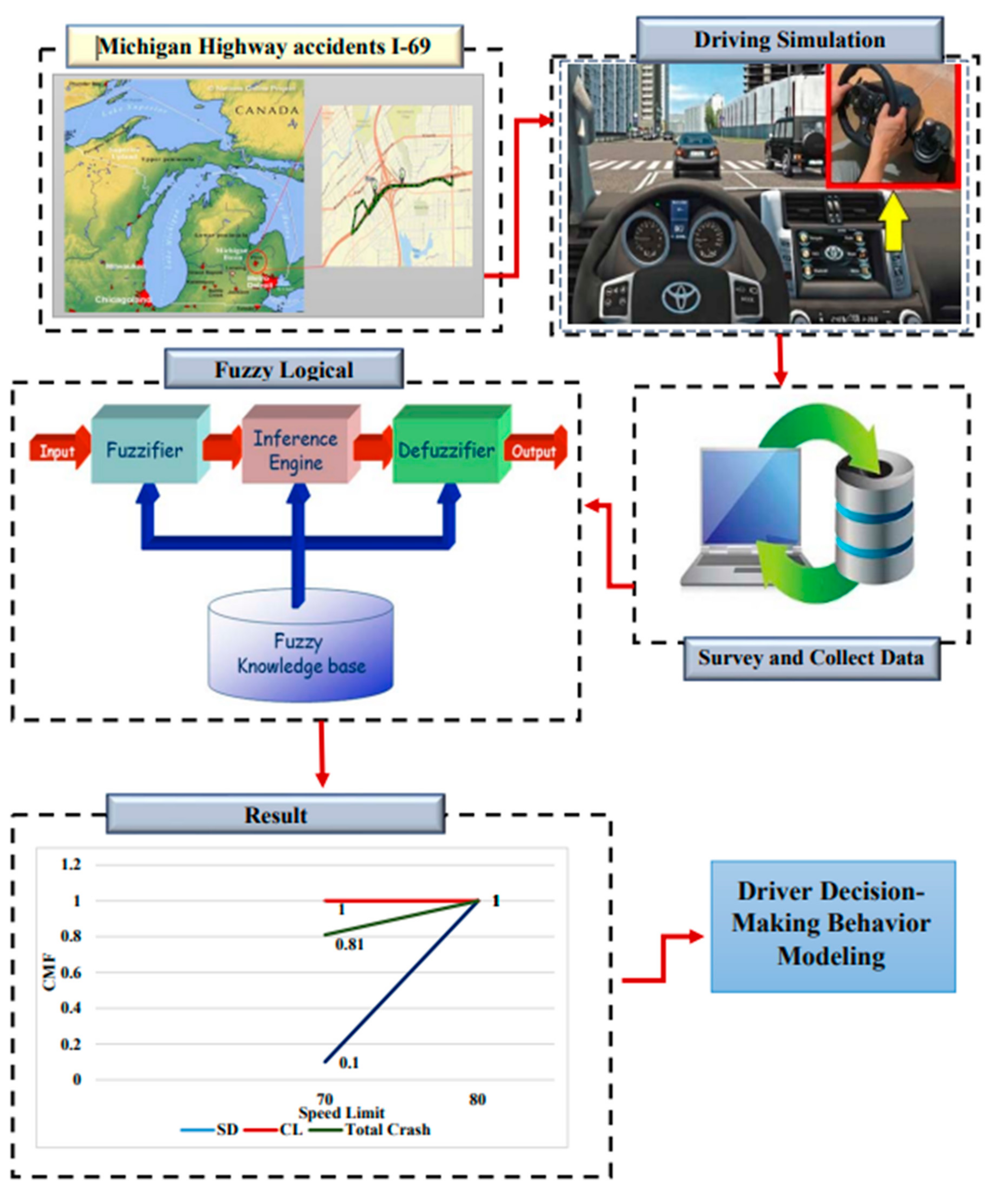
3. Materials and Methods

Driver reporting consists of three main phases: simulation, data collection, and analysis. Firstly, a vehicle speed model based on the simultaneous equations approach is developed and validated with one more site data. Secondly, data collection methods include.surveys, questionnaires, simulations, and realistic experiments. Thirdly, fuzzy logic is applied. A driving simulator provided a safe driving environment for participants, and they were asked to identify changes in the safety effects to establish the best speed limit. As a result of this, participants became more aggressive and exhibited more risk-taking behaviour. As a result, realistic experiments have become an essential and reliable data source. In the analysis phase, the recorded driving data are categorized into labels such as “safe”, “little safe”, “safe”, and “little safe”. Finally, the study methodology followed in the research is presented in Figure 1.

3.1. Data Collection

This study was approved by the Lawrence Technological University (LTU) Institutional Review Board. Additionally, an online training course sponsored by the National Institutes of Health (NIH) Office of extramural research was completed. Subjects were eligible to participate in the study if they had a valid U.S. driver’s license, were 18 years or older, and had driven on an interstate highway in different weather conditions. Data were collected from the driving simulator and a questionnaire answered by participants. Another experiment investigated the avoidance behavior of some middle-aged (31–40) and older participants (51–60) in response to addressing six challenging scenarios on driving simulators. A total of 110 participants, including males and females, were recruited to drive through ten different driving scenarios, 10 for the pilot study and 100 for the experiment design. These drivers ranged from 18 to 60 years old, averaging 35.2 years. Their behavior and reactions to each scenario were captured and evaluated. To evaluate a driver’s compliance with the roadside signs, the study used vehicle speed, lane, braking, total tire slide, and crash information. After analyzing all results, this study proposed a decrease in speed limit from 70 mph to either 50 or 40 mph, especially in icy and snowy road/weather conditions.

3.2. Simulation

This study used a multi-user driving simulator to simulate the above-identified crash types on a virtual I-69 roadway. This crash information, combined with various weather and road conditions, is programmed into the driving simulator as different scenarios. For creating the simulation scenarios, a prototyping approach was used in the driving simulation laboratory at LTU. The driving simulator was designed to contain various driving scenes with the ability to incorporate different road and weather conditions. The driving simulator used in this study included a seat, a computer, a steering wheel, an accelerator, crash, and brakes. The computer screen displayed information for the driver, such as speed in miles per hour (mph), revolutions per minute (rpm), and the driving scenario identification.
The pilot test was performed to assess the scenarios developed for this study to ensure that they include all the data required and are perfect to achieve the study-specific objectives. The scenarios of this pilot test were effectively designed for the driver simulator, considering the differences in participants’ behaviors and differences in road/weather conditions to assist in addressing related questions. The pilot test was a practical way of evaluating the effect of road/weather conditions and speed limits on the participant’s behavior and to enable them to answer the questionnaires concerning their driving experience and safety. Even with a sample size of only 10 participants, the pilot test results justified the designed scenarios and simulator programs and activities, and thus the starting of the experiment design. Realizing the decision-making model of the driver in the driving simulation system. The driving simulation is formed by a vehicle simulation program, a virtual traffic environment, and the virtual driver.

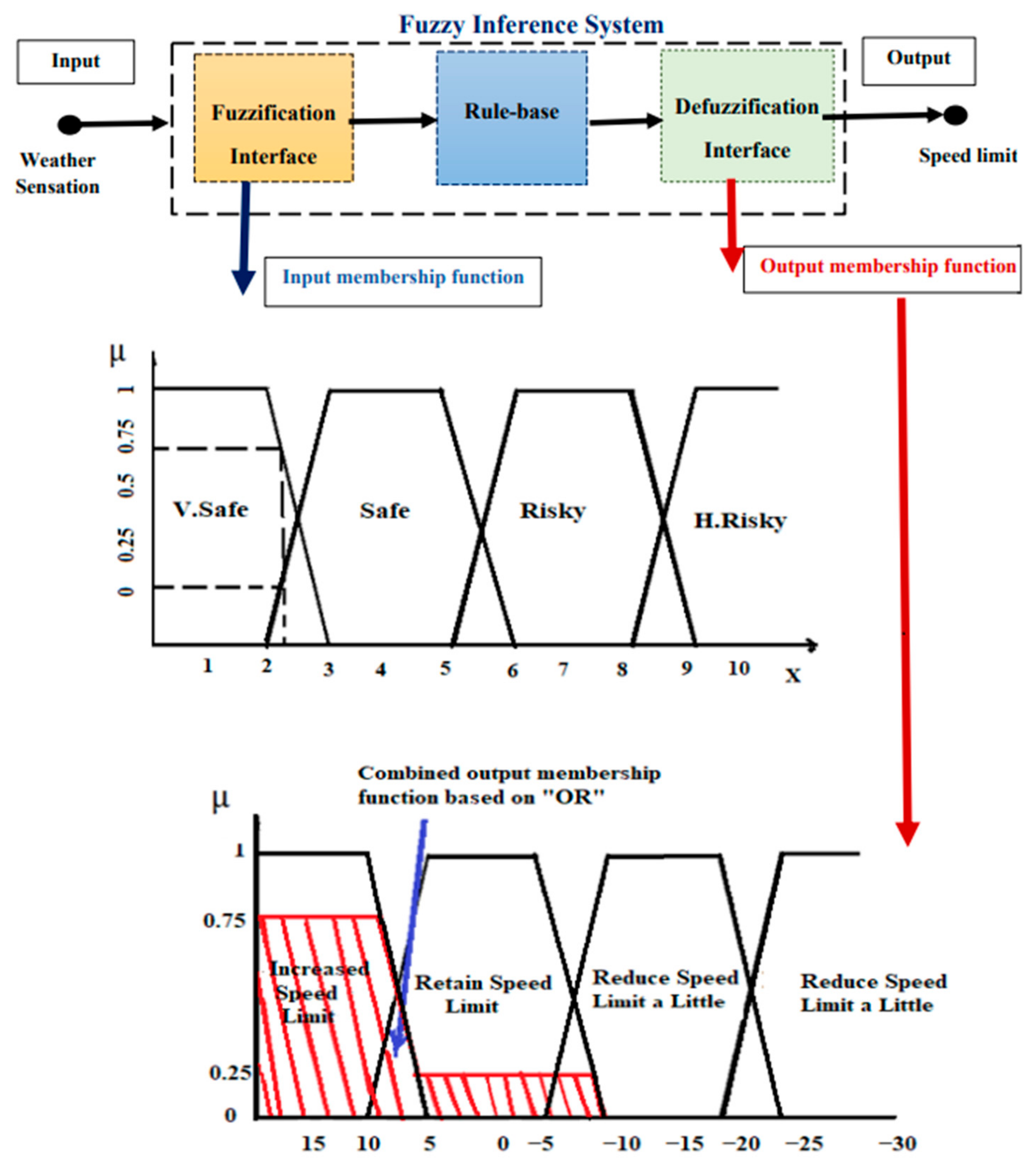
3.3. Short Description of the Fuzzy Inference System

The Fuzzy Logic modeling method is naturally helpful in cases where doubts are complicated. In terms of fuzzy sets, there are different ways to interpret and analyze subjective data from a particular survey case, such as the so-called fuzzy rating scale-based questionnaire. This kind of questionnaire allows expressed human perceptions in fuzzy rating scales. Fuzzy sets were applied to determine each road’s appropriate speed limit and weather conditions. Since the study would be concerned with safety engineers’ subjective judgments, the fuzzy set mathematics is ideal. A fuzzy subset A of a set X is a function A: X → L, where L is the interval [0,1]. This function is also known as the membership function, which is assigned a score ranging between 0 and 1. Fuzzy mathematics was used in answering the questionnaire issued to highway safety engineers to furnish their experience on the rate of speed in different road and weather conditions. Subjectively rated severity levels (very safe, safe, risky, high risky) of each type of weather and road condition were modeled as fuzzy numbers on a scale. Study subject drivers were queried about a possible uncertainty level when rating the severity of a specific type of weather and road condition.
Fuzzy control attempts provide a formal methodology that describes and implements human heuristic knowledge of how to control a system. In this study, we want to control the speed limit to regulate weather sensation. A classical controller would measure weather sensation precisely and compare it with some desired reference and then, based on some model of the speed limit and its impact on weather sensation, it will modify the speed limit. The choice of the membership function shape is not straightforward, and only experience can help the designer.
The primary choice for membership function shapes for this research was the trapezoid, because of its simplicity and linearity that fuzzy logic allows a number or object to be a member of over one set, and it introduces the notion of partial [59]. The general fuzzy inference process is shown in Figure 2, consisting of four components: fuzzy rule base, fuzzy inference process, fuzzification process, and defuzzification [60]. The following is a brief introduction:
Fuzzification
The first stage is fuzzification which represents input variables by converting crisp data values to fuzzy membership functions through fuzzy sets. A fuzzifier operator has the effect of transforming a crisp value into fuzzy sets. The current study considered the crisp inputs from the answers of the subject drivers on each scenario’s questionnaire and then determined the degree to which these inputs belong to each of the appropriate fuzzy sets.
Fuzzy inference process (Aggregation of the Rule Outputs)
The second stage is the inference process, which combines the fuzzy sets of membership functions with the inference rules to obtain the fuzzy output. This step is a process of converting input values into output values using fuzzy logic. Conversion of input into output values is essential for decision-making. Aggregation is the unification process of the outputs of all rules. All rule consequents previously clipped or scaled membership functions are combined into a single fuzzy set.
Defuzzification
The final stage is defuzzification, which represents the output variables based on the fuzzy sets. The Fuzzy Mamdani model for this study is shown in Figure 2. Fuzziness helps us to evaluate the rules; however, the final output of a fuzzy system must be a crisp number. The input for the defuzzification process is the aggregated output fuzzy set, and the output is a single number. The three most important methods are the center of gravity (COG), most significant maximum LOM, and middle of maximum (MOM).
I. 
LOM (largest of maximum), MOM (middle of maximum) methods
The LOM method is based on obtaining the largest of the maximum values as the defuzzification value from the membership functions along with the AND and OR logic operators. However, the MOM method concerns the middle maximum value of the average value in the same zone.
II. 
Center of Gravity method
This method determines the center of the zone that is gained from membership functions with OR logic operators. The formula with which we can calculate the defuzzified crisp output U is given as:
U = M i n M a x µ u * u d u M i n M a x µ u d u
where:
U = The defuzzification result
u = Output variable
µ   = Membership function
M i n = Minimum limit for defuzzification
M a x = Maximum limit for defuzzification
Arianit used three main defuzzification methods: COG, LOM, and MOM. Through this process, it was possible to compare these three defuzzification methods. The results showed crisper values for better link utilization, and the COG method is identified as the best option. Accordingly, this method was used to have better crisp results.
III. 
Crash Modification Factors (CMFs) from Driving Simulator Studies
Identified Crash Modification Factors (CMFs) [61]: “CMFs is a multiplicative factor used to compute the expected number of crashes after implementing a given countermeasure at a specific site. The CMF is multiplied by the expected frequency without treatment”. CMF is a way of evaluating the safety effectiveness of a specific treatment (countermeasure). In other words, it is “the ratio between the number of crashes per unit of time expected after a modification or measure is implemented and the number of crashes per unit of time estimated if the change does not take place”. The application of treatment is said to be effective if a considerable change in safety is felt and recognized; without it, a change could not occur. The estimated crashes with treatment can be determined when the CMF is applied to the estimated crashes without treatment, as described in the following equation:
Estimated   Crashes   WITH   Treatment = CMF × Estimated   WITHOUT   Treatment
A before–after design is conducted, and it compares the number of crash occurrences on the studied part of the road before and after treatment. When a certain countermeasure (treatment) is applied, leading to a CMF less than 1.0, a reduction in crashes is highly anticipated. However, an increase in crashes and a decline in safety are associated with a CMF of more than 1.0. Reconfiguring Equation (3).
CMF = Expected   Crashes   with   treatment   Expected   crashes   without   treatment  
If:
CMF = 1; there is no effect on crash frequency
CMF < 1; crashes are expected to decrease
CMF > 1; crashes are expected to increase
  • Before–After evaluations of performed Studies
Generally, before and after evaluations are performed to develop CMFs for crash reduction countermeasures. Generally, CMFs are developed by analyzing crash data before and after a location countermeasure is applied. This evaluation takes a few years and considerable resources to conduct. There are other issues to be considered for evaluating the quality of CMFs resulting from the before–after designs, and they include the following:Sample Size: The sample size can be determined based on the magnitude of the treatment effect as well as the value of the standard error associated with CMF. The standard error value will decrease with a large sample size and vice versa. Potential Bias: The changes experienced within the periods before and after treatment can be due to undefined factors not included in the proposed countermeasures.These include changes in traffic volume or crash counts. These issues can lead to reduced quality of the resulting CMFs.

4. Results and Discussion

4.1. Descriptive Statistic

In the previous research, a total of 100 individuals were enlisted to participate. To ensure the sample was diverse enough in its gender and age representation. The age of these drivers ranged from 18 to 60 years old. Of the five categories of age groups, the percentage of crash causalities for ages 18–25 was 23%, ages 25–30 was 26%, ages 31–40 was 28%, ages 41–50 was 16%, and ages 51 to 60 was 7%. The percentage of crash causalities for those aged 25–40 was the highest in all five categories. The percentage of male causalities was 81% and 19% for females. Subjects ranged between 18 and 60 years old, 52% had over 10 years of driving experience, and 60% drove using the highway every day. Moreover, 18% of the subjects said they had similarly experienced sliding in their cars when driving in snowy and icy conditions. Fifty-six percent of drivers said that they drove at a speed below the speed limit in clear weather conditions, 9% drove below the speed limit on snow-covered roads, and 9% drove below the speed limit on the highway on snow-covered roads. Safety was classified into three levels (e.g., A Little safe, Less Safe, and Very Safe). When subjects were asked how safe they felt when navigating a highway compared to other roads, 45% felt that they were very safe, 44% felt a little safer, and 11% thought they were less safe. The subjects’ demographic information and driving history are summarized in Table 1.

4.2. Description of the Fuzzy Logic Car-Following Model

The fuzzy logic model controls the system by converting the input and output control variables to linguistic terms representing the fuzzy sets. Using four inference rules through MATLAB, the fuzzy model for this system was constructed using the fuzzy tool, which is the border for developing the expert system. The fuzzy model includes only one input variable and an output variable. Table 2 demonstrates the input and output variables and the inference rules of the model in detail Figure 2, shown below, is an example of weather sensation measurement, or a ‘crisp’ measurement of 2.15. We determined which the values of the membership functions that the crisp measurement gave for each set. The measurement of 2.15 is a member of ‘V. Safe’ to the value of 0.75 and ‘Safe’ to 0.25.
The outputs relating to the inputs ‘V. Safe’ and ‘Safe’ are true to the same degree as the inputs. When applying this process to this study, the 2.15 measurement of 0.75 ‘V. Safe’ and ‘0.25’ Safe results in fuzzy outputs of ‘increase speed’ to the value of 0.75 and ‘Retain speed’ to a value of 0.25. These values truncate the output membership functions, as shown below in Figure 2. The output membership functions are required to be combined into a single membership function. One way to do this is to interpret the combination of two truncated membership functions as an ‘OR’ operator for fuzzy sets.As example of the combined results in an output membership function that looks like this:
μ = 0.75 × 20 + 0.75 × 15 + 0.75 × 10 + 0.25 × 5 + 0.25 × 0 + 0.25 × 5 + 0 × 10 0 + 0.75 + 0.75 + 0.75 + 0.25 + 0.25 + 0.25 + 0 = 11
The output level can vary significantly depending upon the defuzzification method used. For instance, the center of gravity method would yield a value for a change of 11.2 mph. The system outputs the expected values for the output variables. Figure 3 shows the fields where this information is entered (circled in orange) and where the system shows the expected values (circled in green):

4.3. Defuzzification Values and Output for Each Scenario

Table 3 shows the calculated simple average defuzzification for each scenario. The defuzzification values were added and then divided by the total number of observations. The fuzzy rule base employs the fuzzy model results for the inputs of 100 subject drivers from the experimental dataset, which was utilized to assess the performance of the proposed fuzzy model. The fuzzy logic toolbox was used through MATLAB to mirror the control system. This resulted in the specific control of different weather conditions provided by the trapezoidal membership functions. Table 3 shows ranges for all the created fuzzy sets. The ranges for these sets are chosen based on the subject driver’s feelings.
In S1, the conditions were clear weather with an 80 mph speed limit. As shown in Table 3, the speed limit for S1 fluctuated from 5 mph over, or, retaining the current speed, to 20 mph under, or reduced the speed limit. When reviewing the results for S3, the speed limit at 70 mph was retained in the same weather conditions. In S2 and S4, both with rainy weather conditions, the speed limits of 80 mph and 70 mph were retained. However, in S5 and S6, with snowy and icy weather conditions, the speed limit of 70 mph was reduced and ranged from −10 to −20 mph. Similarly, the speed limit was retained in in S7 and S8, with a speed limit of 50 mph and snowy and icy weather conditions. In S9, where there were snowy weather conditions, the speed limit of 40 mph fluctuated between 20 and −5 mph, either retaining this speed limit or increasing the speed limit recommendation. In S10, there were icy weather conditions. Retaining the provided speed limit of 40 mph appeared to provide safe conditions.

4.4. Development of Crash Modification Factors (CMFs) from Driving Simulator Studies

In this study, we used CMF to evaluate the safety and effectiveness of a specific treatment (countermeasure). A before–after design was conducted, and then we compared the number of crash occurrences on the studied part of the road before and after treatment. When a specific countermeasure (treatment) is applied, leading to a CMF of less than 1.0, a reduction in crashes is highly expected. However, an increase in crashes and a decline in safety are associated with a CMF of over 1.0. Generally, before and after evaluations are performed to develop CMFs for crash reduction countermeasures. CMFs are developed by analyzing crash data before and after a location countermeasure is applied. This evaluation takes a few years and considerable resources to conduct. Other issues must be considered for evaluating the quality of CMFs resulting from the before–after designs. The number of estimated crashes for 100 subject drivers in different weather conditions that resulted from the driving simulator experience was used to find the CMF to reduce the number of crashes. This method is called the comparison group method. We estimated the resulting comparison ratio for the “change in mean speed” on the respective weather/road condition before and after the treatment study.Since the before–after designs of CMFs are complicated to develop due to the rationale provided previously, an attempt to develop CMFs using driving simulator studies was performed in this study. Using the previously described data, a change in speed limit during wet, snowy, and icy weather/road conditions was selected as a countermeasure. Table 4 shows the anticipated number of crashes before–after the speed reduction treatment. The suitable and adequate speed limit can be determined using the CMF by considering each weather condition and the speed limit before and after scenarios. Table 4 shows that the number of crashes at the speed limit of 70 mph in snowy weather is 44 and reaches 78 in icy weather conditions. However, when the speed limit is reduced to 50 mph, the number of crashes in snowy weather reaches 15, and, in icy weather, it is 49. The number of crashes decreases when the speed limit is reduced to 40 mph, therefore the crashes reach 4 in snowy weather and 35 in icy weather.
For this study, CMFs are expressed as a numerical value that reflected the expected change in safety. The resulting comparison ratios were estimated for the “change in mean speed” on the respective weather/road condition before and after the treatment study.

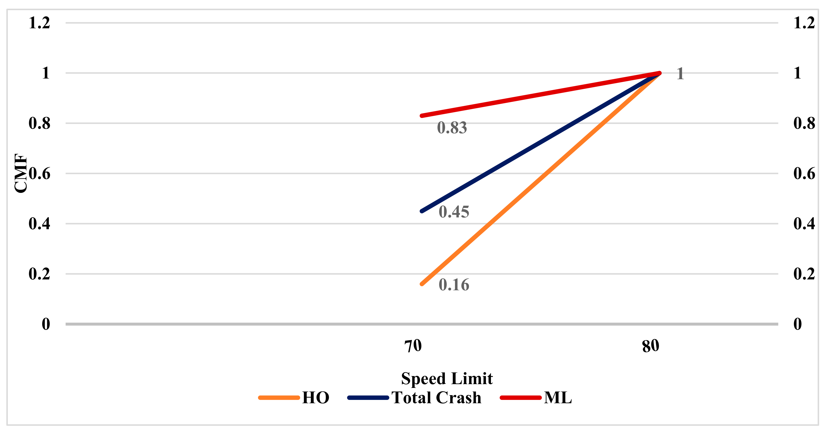
4.4.1. Install Speed Limit in Clear Weather/Dry Road Conditions

The base condition/speed limit of the CMF (i.e., the condition in which the CMF = 1.00) was 80 mph. Changing the speed limit from 80 mph to 70 mph reduced the number of Lane Marge (LM) and Hit Object (HO) road crashes, as shown in Table 5 below. This study also estimated the safety effect of installing a speed limit of 70 mph instead of 80 mph with dry roads and clear weather conditions. Based on the analysis, the implementation of this treatment results in CMF values of 0.83 and 0.16 for LM crashes and HO crashes, respectively.
The researchers found that installing a speed limit of 70 mph instead of 80 mph in dry road conditions results in a CMF of 0.54 for total accidents. Figure 4 shows the relationship between the speed limit and the frequency of events of CMF when the speed limit is decreased by about 10 mph in dry weather/road conditions.

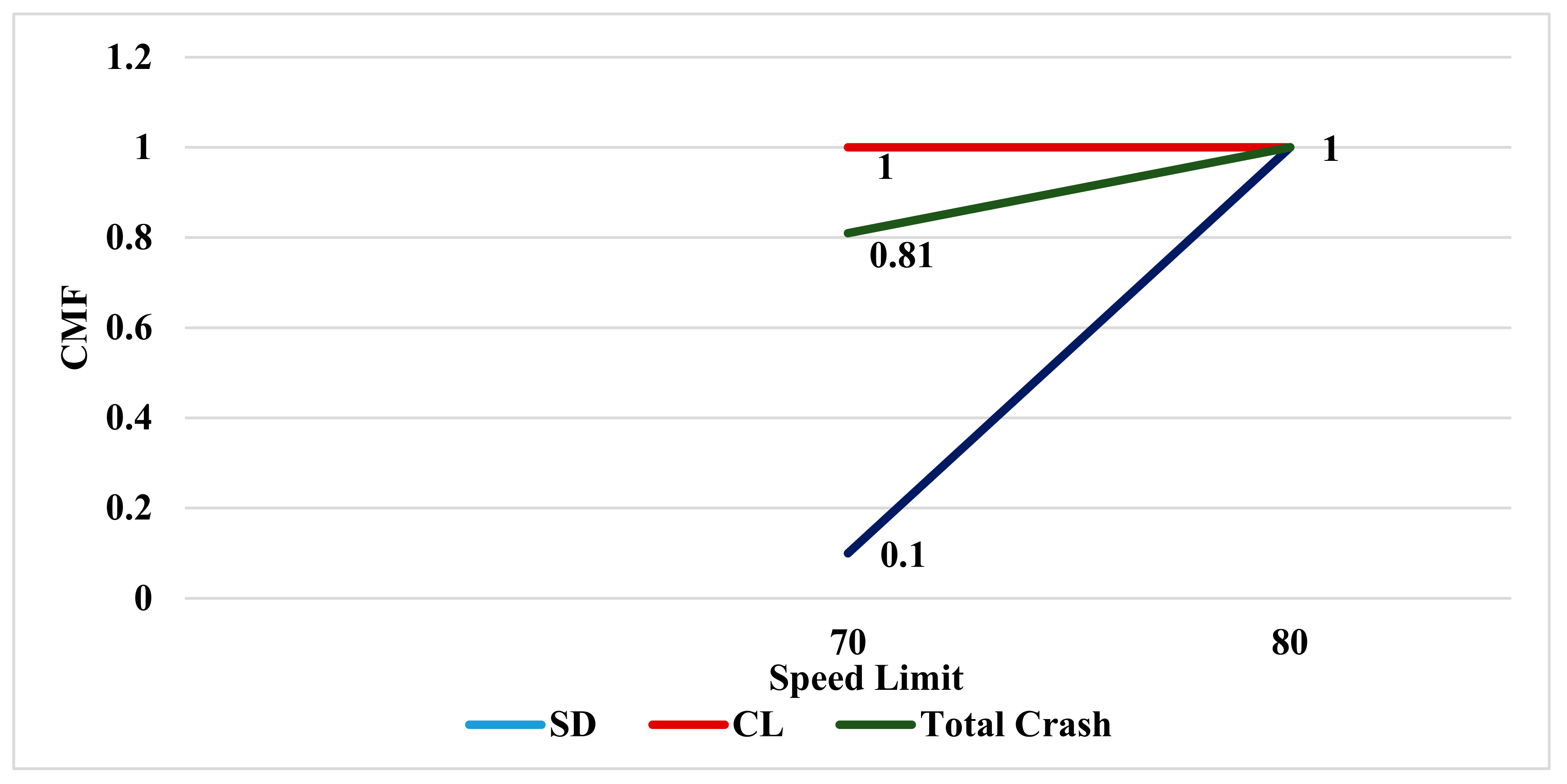
4.4.2. Install Speed Limit for Rain Weather/Wet Road Condition

The crash effects of wet road conditions with a changing speed limit from 80 mph to 70 mph reduced the number of SD crashes, as shown in Table 5. Table 5 illustrates that the speed limit reduction from 80 to 70 mph in rainy weather with wet road conditions was more likely to decrease the expected average SD crash frequencies (CMF = 0.1). However, there was also some frequency events that meant that CL crashes would remain unchanged (CMF = 1). Using the data available from the before–after study, the results show that reducing the speed limit from 80 to 70 mph on the freeway results in a CMF of 0.81 for total crashes. Figure 5 presents the CMF for these potential crashes when modifying the speed limit in wet weather/road conditions. Changing the speed limit during snowy weather reduces crashes due to sliding vehicles. The decision to incorporate speed limit changes in this type of weather may also depend on the road conditions of the actual roadway segment. The road surface effects of the speed limit can be felt in snow and icy conditions. The analysis of crash data for snow weather/snow road conditions found that LOC crashes were more likely to occur in this situation. The reported percentage reduction translates into CMF values of 0.36 and 0.20 for LOC and other crashes, respectively, when reducing the speed limit from 70 mph to 50 mph. Reducing the speed limit from 70 mph to 40 mph resulted in CMF values of 0.03 for LOC crashes and 0.6 for other crashes.

4.4.3. Install Speed Limit in Snow Weather/Snow Road Condition

For the speed limit of 50 mph, the CMF for total crashes applied was 0.43, and, for the speed limit of 40 mph, the CMF for total crashes was 0.09. The results show that the CMFs for total crashes were higher during the speed limit of 50 mph than 40 mph. Figure 5 shows the relationship between the speed limit and the CMF for LOC, other, and total crashes in snow weather/snow road weather conditions.

4.4.4. Install Speed Limit in Snow Weather/Icy Road Conditions

The effects of reducing the speed limit on multilane-divided highways during snowy weather with icy road conditions and a speed limit of 70 mph (CMF = 1) are shown in Table 5. In this scenario, LOC and other road crashes were evaluated. When reducing the speed limit from 70 mph to 50 mph, the resulting CMF was 0.60 for LOC and 1.0 for others. When reducing the speed limit from 70 mph to 40 mph, the CMF was 0.32 for LOC and 0.4 for other crashes. Based on Table 5, by implementing a reduction in speed limit to 50 mph on the freeway, the CMF becomes 0.63 for the total crashes. It is noted that the results of the CMF for the total crashes associated with the speed limit of 40 mph are slightly higher than the CMFs derived for LOC and others and the relationship between the speed limit and the CMF for LOC, others, and total crashes in icy weather/road conditions.

5. Conclusions

The primary aim of this paper was to evaluate different driving styles by developing respective driver models employing a data-driven approach. A fuzzy logic-based framework considering drivers’ decision-making behavior was developed. A safety level was compared to speed limits to determine if the proposed speed limit contributed to a risky or safe driving situation. The final outputs that determined the speed limits for the highway investigated in different road/weather conditions were based on the participants’ responses. The participants could increase or retain their current speed limit or reduce their speed limit a little or significantly under multiple scenarios. The results of the fuzzy logic study suggested the use of a driver’s sensation for predicting outputs. The study results were used to determine the speed limits needed in different road/weather conditions to reduce the number of crashes and implement safe driving conditions based on the weather conditions. The fuzzy logic for this study evaluated how a driver sensed according to the relation between the weather/road condition and the speed limit. The fuzzy logic is expected to contribute to the assessment of a powerful feature of human behavior/controls. The fuzzy logic can explain smooth relationships between the input and output. The input–output relationship estimated by the fuzzy logic was used to understand differences among driver feelings in road/weather conditions at a different speed limits. One of the limitations of this study is that female participants are fewer than male respondents (one-fourth of the sample size). Nevertheless, this uncontrollable factor has limited effects on the model estimation because the sample size is sufficient for the modeling. In future work, more environmental inputs, such as road gradient, time, and weather, can be incorporated to maximize the similarity to diverse drivers population. Moreover, different test drivers’ naturalistic driving data will be collected to formulate more accurate driving style variance. Furthermore, other calibration approaches will also be employed to improve the fuzzy logic controller’s calibration process. Humanized driver models trained using the proposed approach can also be integrated with the decision-making process when designing advanced driver assistance systems (ADAS) and the control strategy of autonomous vehicles.

Author Contributions

Conceptualization, A.I.M.A. and Y.A.; methodology, R.E.A.M., A.I.M.A., Y.A. and I.U.; software, A.I.M.A. and N.B.; validation, I.U., A.J. and Y.A.; formal analysis, R.E.A.M.; investigation, A.I.M.A. and I.U.; resources, Y.A. and A.J.; data curation, A.J. and N.B.; writing—original draft preparation, A.I.M.A., I.U. and N.B.; writing—review and editing, Y.A. and A.J.; visualization, R.E.A.M. and A.J.; supervision, Y.A. and R.E.A.M.; project administration, Y.A.; funding acquisition, Y.A. and A.J. All authors have read and agreed to the published version of the manuscript.

Funding

This project was funded by the Deanship of Scientific Research (DSR) at King Abdulaziz University, Jeddah (Grant No. RG-21-140-42). The authors gratefully acknowledge the DSR fortechnical and financial support. The DSR had no role in the design of the study, data collection, dataanalysis, interpretation of data, or writing of the article. Availability of data and materials. The datasets used and/or analyzed during the current study are available from the corresponding authorupon request.

Institutional Review Board Statement

The study was conducted in accordance with the approval by the Institutional Review Board of Lawrence Technological University. The motives/aims of the study were told to respondents with respect to the survey. They were also assured about of their anonymity and confidentiality in their responses. Their participation was absolutely voluntary, and they are not compensated.

Informed Consent Statement

Informed consent was obtained from all subjects involved in the study.

Data Availability Statement

All accompanying data are provided in the manuscript.

Acknowledgments

The authors acknowledge and appreciate the support Lawrence Technological University and King Abdulaziz University (KAU) for supporting this study.

Conflicts of Interest

The authors declare no conflict of interest.

References

  1. Feraud, I.S.; Naranjo, J.E. Are You a Good Driver? A Data-Driven Approach to Estimate Driving Style. In Proceedings of the 11th International Conference on Computer Modeling and Simulation, New York, NY, USA, 16–19 January 2019; pp. 3–7. [Google Scholar]
  2. Petridou, E.; Moustaki, M. Human Factors in the Causation of Road Traffic Crashes. Eur. J. Epidemiol. 2000, 16, 819–826. [Google Scholar] [CrossRef] [PubMed]
  3. Driving, A. Research Update; AAA Foundation for Traffic Safety: Washington, DC, USA, 2009. [Google Scholar]
  4. Tasca, L. A Review of the Literature on Aggressive Driving Research; Citeseer: Princeton, NJ, USA, 2000. [Google Scholar]
  5. Safdar, M.; Jamal, A.; Al-Ahmadi, H.M.; Rahman, M.T.; Almoshaogeh, M. Analysis of the Influential Factors towards Adoption of Car-Sharing: A Case Study of a Megacity in a Developing Country. Sustainability 2022, 14, 2778. [Google Scholar] [CrossRef]
  6. Wang, Z.; Safdar, M.; Zhong, S.; Liu, J.; Xiao, F. Public Preferences of Shared Autonomous Vehicles in Developing Countries: A Cross-National Study of Pakistan and China. J. Adv. Transp. 2021, 2021, 5141798. [Google Scholar] [CrossRef]
  7. Meiring, G.A.M.; Myburgh, H.C. A Review of Intelligent Driving Style Analysis Systems and Related Artificial Intelligence Algorithms. Sensors 2015, 15, 30653–30682. [Google Scholar] [CrossRef] [PubMed]
  8. Johnson, D.A.; Trivedi, M.M. Driving Style Recognition Using a Smartphone as a Sensor Platform. In Proceedings of the 2011 14th International IEEE Conference on Intelligent Transportation Systems (ITSC), Washington, DC, USA, 5–7 October 2011; pp. 1609–1615. [Google Scholar]
  9. Jamal, A.; Rahman, M.T.; Al-Ahmadi, H.M.; Mansoor, U. The Dilemma of Road Safety in the Eastern Province of Saudi Arabia: Consequences and Prevention Strategies. Int. J. Environ. Res. Public Health 2020, 17, 157. [Google Scholar] [CrossRef] [PubMed] [Green Version]
  10. Sagberg, F.; Selpi; Bianchi Piccinini, G.F.; Engström, J. A Review of Research on Driving Styles and Road Safety. Hum. Factors 2015, 57, 1248–1275. [Google Scholar] [CrossRef]
  11. Harris, P.B.; Houston, J.M.; Vazquez, J.A.; Smither, J.A.; Harms, A.; Dahlke, J.A.; Sachau, D.A. The Prosocial and Aggressive Driving Inventory (PADI): A Self-Report Measure of Safe and Unsafe Driving Behaviors. Accid. Anal. Prev. 2014, 72, 1–8. [Google Scholar] [CrossRef] [PubMed]
  12. Houston, J.M.; Harris, P. The Aggressive Driving Behavior Scale: Developing a Self-Report Measure of Unsafe Driving Practices. N. Am. J. Psychol. 2003, 5, 193–202. [Google Scholar]
  13. Dula, C.S.; Ballard, M.E. Development and Evaluation of a Measure of Dangerous, Aggressive, Negative Emotional, and Risky Driving 1. J. Appl. Soc. Psychol. 2003, 33, 263–282. [Google Scholar] [CrossRef]
  14. Krahé, B.; Fenske, I. Predicting Aggressive Driving Behavior: The Role of Macho Personality, Age, and Power of Car. Aggress. Behav. Off. J. Int. Soc. Res. Aggress. 2002, 28, 21–29. [Google Scholar] [CrossRef]
  15. Ullah, I.; Liu, K.; Yamamoto, T.; Zahid, M.; Jamal, A. Prediction of Electric Vehicle Charging Duration Time Using Ensemble Machine Learning Algorithm and Shapley Additive Explanations. Int. J. Energy Res. 2022, in press. [CrossRef]
  16. Ullah, I.; Liu, K.; Yamamoto, T.; Al Mamlook, R.E.; Jamal, A. A Comparative Performance of Machine Learning Algorithm to Predict Electric Vehicles Energy Consumption: A Path towards Sustainability. Energy Environ. 2021, 0958305X211044998. [Google Scholar] [CrossRef]
  17. Ali Aden, W.; Zheng, J.; Ullah, I.; Safdar, M. Public Preferences Towards Car Sharing Service: The Case of Djibouti. Front. Environ. Sci. 2022, 10, 889453. [Google Scholar] [CrossRef]
  18. Aljaafreh, A.; Alshabatat, N.; Al-Din, M.S.N. Driving Style Recognition Using Fuzzy Logic. In Proceedings of the 2012 IEEE International Conference on Vehicular Electronics and Safety (ICVES 2012), Istanbul, Turkey, 24–27 July 2012; pp. 460–463. [Google Scholar]
  19. WÅhlberg, A.A. Driver Behaviour and Accident Research Methodology: Unresolved Problems; CRC Press: Boca Raton, FL, USA, 2017. [Google Scholar]
  20. Jamal, A.; Umer, W. Exploring the Injury Severity Risk Factors in Fatal Crashes with Neural Network. Int. J. Environ. Res. Public Health 2020, 17, 7466. [Google Scholar] [CrossRef] [PubMed]
  21. Jamal, A.; Zahid, M.; Tauhidur Rahman, M.; Al-Ahmadi, H.M.; Almoshaogeh, M.; Farooq, D.; Ahmad, M. Injury Severity Prediction of Traffic Crashes with Ensemble Machine Learning Techniques: A Comparative Study. Int. J. Inj. Control. Saf. Promot. 2021, 28, 408–427. [Google Scholar] [CrossRef]
  22. Wang, W.; Xi, J. A Rapid Pattern-Recognition Method for Driving Styles Using Clustering-Based Support Vector Machines. In Proceedings of the 2016 American Control Conference (ACC), Boston, MA, USA, 6–8 July 2016; pp. 5270–5275. [Google Scholar]
  23. Feng, Y.; Pickering, S.; Chappell, E.; Iravani, P.; Brace, C. A Support Vector Clustering Based Approach for Driving Style Classification. Int. J. Mach. Learn. Comput. 2019, 9, 344–350. [Google Scholar] [CrossRef] [Green Version]
  24. Li, G.; Chen, Y.; Cao, D.; Qu, X.; Cheng, B.; Li, K. Extraction of Descriptive Driving Patterns from Driving Data Using Unsupervised Algorithms. Mech. Syst. Signal Process. 2021, 156, 107589. [Google Scholar] [CrossRef]
  25. Li, G.; Li, S.E.; Cheng, B.; Green, P. Estimation of Driving Style in Naturalistic Highway Traffic Using Maneuver Transition Probabilities. Transp. Res. Part C Emerg. Technol. 2017, 74, 113–125. [Google Scholar] [CrossRef]
  26. Tulusan, J.; Staake, T.; Fleisch, E. Providing Eco-Driving Feedback to Corporate Car Drivers: What Impact Does a Smartphone Application Have on Their Fuel Efficiency? In Proceedings of the 2012 ACM Conference on Ubiquitous Computing, Pittsburgh, PA, USA, 5–8 September 2012; pp. 212–215. [Google Scholar]
  27. Staubach, M.; Schebitz, N.; Köster, F.; Kuck, D. Evaluation of an Eco-Driving Support System. Transp. Res. Part F Traffic Psychol. Behav. 2014, 27, 11–21. [Google Scholar] [CrossRef]
  28. Sullman, M.J.; Dorn, L.; Niemi, P. Eco-Driving Training of Professional Bus Drivers—Does It Work? Transp. Res. Part C Emerg. Technol. 2015, 58, 749–759. [Google Scholar] [CrossRef]
  29. Deffenbacher, J.L.; Oetting, E.R.; Lynch, R.S. Development of a Driving Anger Scale. Psychol. Rep. 1994, 74, 83–91. [Google Scholar] [CrossRef] [PubMed]
  30. De Winter, J.C.; Dodou, D. The Driver Behaviour Questionnaire as a Predictor of Accidents: A Meta-Analysis. J. Saf. Res. 2010, 41, 463–470. [Google Scholar] [CrossRef] [PubMed]
  31. Amado, S.; Arıkan, E.; Kaça, G.; Koyuncu, M.; Turkan, B.N. How Accurately Do Drivers Evaluate Their Own Driving Behavior? An on-Road Observational Study. Accid. Anal. Prev. 2014, 63, 65–73. [Google Scholar] [CrossRef]
  32. Osafune, T.; Takahashi, T.; Kiyama, N.; Sobue, T.; Yamaguchi, H.; Higashino, T. Analysis of Accident Risks from Driving Behaviors. Int. J. Intell. Transp. Syst. Res. 2017, 15, 192–202. [Google Scholar] [CrossRef]
  33. Koh, D.-W.; Kang, H.-B. Smartphone-Based Modeling and Detection of Aggressiveness Reactions in Senior Drivers. In Proceedings of the 2015 IEEE Intelligent Vehicles Symposium (IV), Seoul, Korea, 28 June–1 July 2015; pp. 12–17. [Google Scholar]
  34. Hong, J.-H.; Margines, B.; Dey, A.K. A Smartphone-Based Sensing Platform to Model Aggressive Driving Behaviors. In Proceedings of the Sigchi Conference on Human Factors in Computing Systems, Toronto, ON, Canada, 26 April–1 May 2014; pp. 4047–4056. [Google Scholar]
  35. Yoshitake, H.; Shino, M. Risk Assessment Based on Driving Behavior for Preventing Collisions with Pedestrians When Making Across-Traffic Turns at Intersections. IATSS Res. 2018, 42, 240–247. [Google Scholar] [CrossRef]
  36. Af Wåhlberg, A.E. The Relation of Acceleration Force to Traffic Accident Frequency: A Pilot Study. Transp. Res. Part F Traffic Psychol. Behav. 2000, 3, 29–38. [Google Scholar] [CrossRef]
  37. Xu, W.; Wang, J.; Fu, T.; Gong, H.; Sobhani, A. Aggressive Driving Behavior Prediction Considering Driver’s Intention Based on Multivariate-Temporal Feature Data. Accid. Anal. Prev. 2022, 164, 106477. [Google Scholar] [CrossRef]
  38. Karlaftis, M.G.; Vlahogianni, E.I. Memory Properties and Fractional Integration in Transportation Time-Series. Transp. Res. Part C Emerg. Technol. 2009, 17, 444–453. [Google Scholar] [CrossRef]
  39. Zhong, M.; Lingras, P.; Sharma, S. Estimation of Missing Traffic Counts Using Factor, Genetic, Neural, and Regression Techniques. Transp. Res. Part C Emerg. Technol. 2004, 12, 139–166. [Google Scholar] [CrossRef]
  40. Van Der Voort, M.; Dougherty, M.; Watson, S. Combining Kohonen Maps with ARIMA Time Series Models to Forecast Traffic Flow. Transp. Res. Part C Emerg. Technol. 1996, 4, 307–318. [Google Scholar] [CrossRef] [Green Version]
  41. Williams, B.M.; Hoel, L.A. Modeling and Forecasting Vehicular Traffic Flow as a Seasonal ARIMA Process: Theoretical Basis and Empirical Results. J. Transp. Eng. 2003, 129, 664–672. [Google Scholar] [CrossRef] [Green Version]
  42. Al Mamlook, R.E.; Abdulhameed, T.Z.; Hasan, R.; Al-Shaikhli, H.I.; Mohammed, I.; Tabatabai, S. Utilizing Machine Learning Models to Predict the Car Crash Injury Severity among Elderly Drivers. In Proceedings of the 2020 IEEE international conference on electro information technology (EIT), Chicago, IL, USA, 31 July–1 August 2020; pp. 105–111. [Google Scholar]
  43. Habtemichael, F.G.; Cetin, M. Short-Term Traffic Flow Rate Forecasting Based on Identifying Similar Traffic Patterns. Transp. Res. Part C Emerg. Technol. 2016, 66, 61–78. [Google Scholar] [CrossRef]
  44. Chan, K.Y.; Dillon, T.S.; Singh, J.; Chang, E. Neural-Network-Based Models for Short-Term Traffic Flow Forecasting Using a Hybrid Exponential Smoothing and Levenberg-Marquardt Algorithm. IEEE Trans. Intell. Transp. Syst. 2011, 13, 644–654. [Google Scholar] [CrossRef]
  45. Vlahogianni, E.I.; Karlaftis, M.G.; Golias, J.C. Optimized and Meta-Optimized Neural Networks for Short-Term Traffic Flow Prediction: A Genetic Approach. Transp. Res. Part C Emerg. Technol. 2005, 13, 211–234. [Google Scholar] [CrossRef]
  46. Zheng, W.; Lee, D.-H.; Shi, Q. Short-Term Freeway Traffic Flow Prediction: Bayesian Combined Neural Network Approach. J. Transp. Eng. 2006, 132, 114–121. [Google Scholar] [CrossRef] [Green Version]
  47. Dimitriou, L.; Tsekeris, T.; Stathopoulos, A. Adaptive Hybrid Fuzzy Rule-Based System Approach for Modeling and Predicting Urban Traffic Flow. Transp. Res. Part C Emerg. Technol. 2008, 16, 554–573. [Google Scholar] [CrossRef]
  48. Tan, M.-C.; Wong, S.C.; Xu, J.-M.; Guan, Z.-R.; Zhang, P. An Aggregation Approach to Short-Term Traffic Flow Prediction. IEEE Trans. Intell. Transp. Syst. 2009, 10, 60–69. [Google Scholar]
  49. Roozbeh, M.; Hesamian, G.; Akbari, M.G. Ridge Estimation in Semi-Parametric Regression Models under the Stochastic Restriction and Correlated Elliptically Contoured Errors. J. Comput. Appl. Math. 2020, 378, 112940. [Google Scholar] [CrossRef]
  50. Kumar, M.K.; Prasad, V.K. Driver Behavior Analysis and Prediction Models: A Survey. Int. J. Comput. Sci. Inf. Technol. 2015, 6, 3328–3333. [Google Scholar]
  51. Moslem, S.; Farooq, D.; Ghorbanzadeh, O.; Blaschke, T. Application of the AHP-BWM Model for Evaluating Driver Behavior Factors Related to Road Safety: A Case Study for Budapest. Symmetry 2020, 12, 243. [Google Scholar] [CrossRef] [Green Version]
  52. De Oña, J.; de Oña, R.; Eboli, L.; Forciniti, C.; Mazzulla, G. How to Identify the Key Factors That Affect Driver Perception of Accident Risk. A Comparison between Italian and Spanish Driver Behavior. Accid. Anal. Prev. 2014, 73, 225–235. [Google Scholar] [CrossRef] [PubMed]
  53. Liu, J.; Wang, C.; Liu, Z.; Feng, Z.; Sze, N.N. Drivers’ Risk Perception and Risky Driving Behavior under Low Illumination Conditions: Modified Driver Behavior Questionnaire (DBQ) and Driver Skill Inventory (DSI). J. Adv. Transp. 2021, 2021, 5568240. [Google Scholar] [CrossRef]
  54. Ross, T.J. Fuzzy Logic with Engineering Applications; John Wiley & Sons: Hoboken, NJ, USA, 2005. [Google Scholar]
  55. Guney, K.; Sarikaya, N. Comparison of Mamdani and Sugeno Fuzzy Inference System Models for Resonant Frequency Calculation of Rectangular Microstrip Antennas. Prog. Electromagn. Res. B 2009, 12, 81–104. [Google Scholar] [CrossRef] [Green Version]
  56. Jassbi, J.J.; Serra, P.J.; Ribeiro, R.A.; Donati, A. A Comparison of Mandani and Sugeno Inference Systems for a Space Fault Detection Application. In Proceedings of the 2006 World Automation Congress, Budapest, Hungary, 24–26 July 2006; pp. 1–8. [Google Scholar]
  57. Dörr, D.; Grabengiesser, D.; Gauterin, F. Online Driving Style Recognition Using Fuzzy Logic. In Proceedings of the 17th international IEEE conference on intelligent transportation systems (ITSC), Qingdao, China, 8–11 October 2014; pp. 1021–1026. [Google Scholar]
  58. Hao, H.; Ma, W.; Xu, H. A Fuzzy Logic-Based Multi-Agent Car-Following Model. Transp. Res. Part C Emerg. Technol. 2016, 69, 477–496. [Google Scholar] [CrossRef]
  59. Klir, G.; Yuan, B. Fuzzy Sets and Fuzzy Logic; Prentice Hall New Jersey: Hoboken, NJ, USA, 1995; Volume 4. [Google Scholar]
  60. Yadav, O.P.; Singh, N.; Chinnam, R.B.; Goel, P.S. A Fuzzy Logic Based Approach to Reliability Improvement Estimation during Product Development. Reliab. Eng. Syst. Saf. 2003, 80, 63–74. [Google Scholar] [CrossRef]
  61. Gross, F.; Persaud, B.N.; Lyon, C. A Guide to Developing Quality Crash Modification Factors; Federal Highway Administration, Office of Safety: Washington, DC, USA, 2010. [Google Scholar]
Figure 1. Study methodology.
Sustainability 14 08874 g001
Figure 2. Fuzzy Mamdani model.
Sustainability 14 08874 g002
Figure 3. Expert system operation.
Sustainability 14 08874 g003
Figure 4. The relationship between the speed limit and CMF in dry weather/road condition.
Sustainability 14 08874 g004
Figure 5. The relationship between the speed limit and CMF in wet weather/road conditions.
Sustainability 14 08874 g005
Table 1. Descriptive statistics of pre-experiment questionnaire.
Driver CharacteristicsClassificationProportion of Drivers
Age(18–25)23%
(25–30)26%
(31–40)28%
(41–50)16%
(51–60)7%
GenderMale81%
Female19%
No. of years of driving experiencePrimary (1–5 years)27%
Middle (6–9 years)21%
Senior (≥10 years)52%
Highway driving mileage per dayEvery day60%
Occasionally12%
Often28%
Speed when you drive on a highway on snow-covered roadsSimilar18%
Below speed limit56%
Below speed 10 limit17%
Below 5 mph9%
Number of times the driver has slid on snowy and icy roads Sometimes60%
Never12%
Often28%
SafetyA Little Safe44%
Less Safe11%
Very Safe45%
Table 2. Description of variables, mathematical representation, their fuzzy sets, and rules.
VariablesMathematical RepresentationGeneralized Trapezoidal Fuzzy
Weather Sensation (Input)
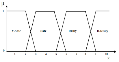
 µ V . S a f e x = 0 ;           x 3 Sustainability 14 08874 i001
µ V . S a f e x = X 2 3 2 ;     2 < x < 3
µ V . S a f e x = 1 ;             x 2
µ S a f e x = 0 ;           x 6
µ S a f e x = X 5 6 5 ;     5 < x < 6
µ S a f e x = 1 ;             x 5
µ R i s k y x = 0 ;           x 9
µ R i s k y x = X 8 9 8 ;     8 < x < 9
µ R i s k y x = 1 ;             x 8
µ H . R i s k y x = 0 ;           x 10 Fuzzy SetsVery safesafeRiskyHigh, Risky
µ H . R i s k y x = X 9 10 9 ;     9 < x < 10 Values0–1–2–32–3–4–55–6–7–88–9–10
µ H . R i s k y x = 1 ;             x 9
Speed Limit (Output) µ I . S p e e d x = 0 ;           x 5 Sustainability 14 08874 i002
µ I . S p e e d x = 10 X 10 5 ;     10 > x < 5
µ I . S p e e d x = 1 ;   x 10
µ R e t a i n   . S p e e d x = 0 ;           x 10
µ R e t a i n   . S p e e d x = 5 x 5 10 ; 5 > x < 10
µ R e t a i n   . S p e e d x = 1 ;             x 5
µ R e d u c e   a   l e t t e l x = 0 ;           x 25
µ R e d u c e   a   l e t t e l x = 20 x ( 20 25 20 > x < 25 Fuzzy Setsincrease the speed limitretain current the speed limitreduce the speed limit a littlereduce the speed limit a lot
µ R e d u c e   a   l e t t e l x = 1 ;             x 20
µ R e d u c e   a   l o t x = 0 ;           x 30 Values20–15–10–510–5–0–(−5)(−5)–(10)–(−15)–(20)(−20)–(25)–(30)
µ R e d u c e   a   l o t x = 25 x 25 30 ; 25 > x > 30
µ R e d u c e   a   l o t x = 1 ;     x 25
Production Rules:
If the weather sensation is Very Safe, then increase the speed limit.
If the weather sensation is Safe, then retain current the speed limit.
If weather sensation is Risky, then reduce the speed limit a little.
If the weather sensation is High Risky, then reduce the speed limit a lot.
Note: The part of the rule that precedes the ‘then’ is termed the antecedent part, whilst the part of the rule that follows the ‘then’ is termed the consequent part.
Table 3. The defuzzification values and output for each scenario.
ScenarioWeather Condition/Speed LimitAverage DefuzzificationModify the Speed LimitSpeed Range (mph)
S1Clear/80 mph−5.3195the speed limit/reduce the speedFrom 5 to −20
S2Rain/80 mph−3.8166retain the current speed limitFrom 5 to −5
S3Clear/70 mph−0.3513retain the current speed limitFrom 5 to −5
S4Rain/70 mph2.0397retain the current speed limitFrom 5 to −5
S5Snow/70 mph−11.492reduce the speed limit a littleFrom −10 to −20
S6Icy/70 mph−16.4599reduce the speed limit a littleFrom −10 to −20
S7Snow/50 mph1.4335retain the current speed limitFrom 5 to −5
S8Icy/50 mph−3.9219retain the current speed limitFrom 5 to −5
S9Snow/40 mph6.6224increase the speed limit/speed limitFrom 20 to −5
S10Icy/40mph3.4828retain current the speed limitFrom 5 to −5
Table 4. Crash data for before–after treatment for 100 subject drivers.
Weather/Road ConditionTime PeriodChange Speed LimitCrash TypeCount
Clear/dryBefore80 mphLane Marge (LM)18
Hit Object (HO)24
After70 mphLane Marge (LM)15
Hit Object (HO)4
Rain/wetBefore80 mphSlow Dawn (SD)10
Loss of Control (LOC)11
After70 mphSlow Dawn (SD6
Lane Change (CL)11
Snow/snowBefore70 mphLoss of Control (LOC)39
OTHER5
After50 mphLoss of Control (LOC)14
OTHER1
After40 mphLoss of Control (LOC)1
OTHER3
Snow/icyBefore70 mphLoss of Control (LOC)73
OTHER5
After50 mphLoss of Control (LOC)44
OTHER5
After40 mphLoss of Control (LOC)23
OTHER2
Hit Deer (HD)10
Table 5. Potential crash effects of speed change on highways for related crash types.
No #TreatmentTraffic VolumeTraffic VolumeWeather/Road ConditionCMF
Speed limit and CMF in Clear/dry conditionLMHOTotal CrashStd. Error
1Change mean speed from 80 mph to 70 mphFreeway (Four-lane roads)UnspecifiedClear/dry0.830.160.450.047
Speed limit and CMF in Cloudy/wet conditionSDCLTotal CrashStd. Error
2Change mean speed from 80 mph to 70 mphFreeway (Four-lane roads)UnspecifiedCloudy/wet0.110.810.046
Speed limit and CMF in Snow/snow conditionLOCOtherTotal CrashStd. Error
3Change mean speed from 70 mph to 50 mphFreeway (Four-lane roads)UnspecifiedSnow/snow0.360.200.430.037
Change mean speed from 70 mph to 40 mph0.030.600.090.038
Speed limit and CMF in Snow/icy conditionLOCOtherTotal CrashStd. Error
4Change mean speed from 70 mph to 50 mphFreeway (Four-lane roads)UnspecifiedSnow/icy0.601.00.630.040
Change mean speed from 70 mph to 40 mph0.320.400.450.053
Publisher’s Note: MDPI stays neutral with regard to jurisdictional claims in published maps and institutional affiliations.

