Article

An Adaptive Multi-Level Quantization-Based Reinforcement Learning Model for Enhancing UAV Landing on Moving Targets

1
Research Center for Unmanned Vehicles, Faculty of Mechanical and Manufacturing Engineering, Universiti Tun Hussein Onn Malaysia, Parit Raja, Batu Pahat 86400, Johor, Malaysia
2
Faculty of Computer Science and Information Technology, Universiti Tun Hussin Onn Malaysia, Parit Raja, Batu Pahat 84600, Johor, Malaysia
3
College of Technological Innovation, Zayed University, Abu Dhabi 4783, United Arab Emirates
4
Faculty of Electrical and Electronic Engineering, Universiti Tun Hussein Onn Malaysia, Parit Raja, Batu Pahat 86400, Johor, Malaysia
5
College of Computer Science and Information Technology, University of Anbar, Ramadi 31001, Iraq
6
Department of Medical Instrumentation Techniques Engineering, Al-Mustaqbal University College, Hillah 51001, Iraq
7
Department of Medical Instruments Engineering Techniques, Dijlah University College, Baghdad 10021, Iraq
8
Department of Medical Instruments Engineering Techniques, Al-Farahidi University, Baghdad 10021, Iraq
9
Department of Electrical Engineering, Faculty of Engineering, Universiti Malaya, Kuala Lumpur 50603, Selangor, Malaysia
*
Authors to whom correspondence should be addressed.
Sustainability 2022, 14(14), 8825; https://doi.org/10.3390/su14148825
Submission received: 30 April 2022 / Revised: 8 July 2022 / Accepted: 14 July 2022 / Published: 19 July 2022

Abstract

:
The autonomous landing of an unmanned aerial vehicle (UAV) on a moving platform is an essential functionality in various UAV-based applications. It can be added to a teleoperation UAV system or part of an autonomous UAV control system. Various robust and predictive control systems based on the traditional control theory are used for operating a UAV. Recently, some attempts were made to land a UAV on a moving target using reinforcement learning (RL). Vision is used as a typical way of sensing and detecting the moving target. Mainly, the related works have deployed a deep-neural network (DNN) for RL, which takes the image as input and provides the optimal navigation action as output. However, the delay of the multi-layer topology of the deep neural network affects the real-time aspect of such control. This paper proposes an adaptive multi-level quantization-based reinforcement learning (AMLQ) model. The AMLQ model quantizes the continuous actions and states to directly incorporate simple Q-learning to resolve the delay issue. This solution makes the training faster and enables simple knowledge representation without needing the DNN. For evaluation, the AMLQ model was compared with state-of-art approaches and was found to be superior in terms of root mean square error (RMSE), which was 8.7052 compared with the proportional–integral–derivative (PID) controller, which achieved an RMSE of 10.0592.

1. Introduction

Unmanned aerial vehicle (UAV) applications are increasing daily and are part of many recent technological applications. Some examples of UAV or drone applications are shipping [1], surveillance [2,3], battlefield [4], rescuing applications [5,6], inspection [7,8], tracking [3], etc. One of the appealing applications of UAVs is traffic sensing [9] and congestion estimation [10], and/or detection, which is beneficial for intelligent transportation systems (ITS) [11]. The UAV has the advantage of having no humans on board, making it a fixable and desirable platform for exploring and applying new ideas. Subsequently, UAV technology has opened the door to many sustainability-related studies, including agriculture, air quality, fire control, pollen count, etc.
The UAV’s control system is categorized into three parts: teleoperated [12,13], semi-autonomous [14,15], and full autonomous [7,16]. Each category defines the involvement level of humans in UAV flight control and daily activities. The sustainability of UAV applications requires essential autonomous features that provide a high degree of autonomy in the UAV systems. These autonomous features improve the UAV’s performance in complex environments and sustain its safety. One essential autonomous feature is auto-landing on a moving target. In various applications such as ground-aerial vehicle collaboration, aerial vehicles need to identify a certain landing area. This functionality has to be autonomous because of the challenging aspect of the teleoperation when landing on a moving target. In addition, there is a risk of failure, which might cause damage to the aerial vehicle and other properties. It is necessary to include the functionality of autonomous landing in all categories of the operation of UAVs, even in the teleoperation category. Hence, the landing of UAVs on moving targets is an essential function of robotics competitions [17,18]. The UAVs have a limited flight time. When the targeted task is far from the ground station, one solution is to use a mobile carrier such as a truck, helicopter, or ship. For example, a flight landing on a moving ship deck requires identifying the landing spot and assuring a safe and precise landing while the ship is moving [19].
The mathematical function of the plant is important for ensuring a reliable controller in nonlinear and dynamic control systems. The controller’s stability is assessed using complex mathematical approaches and techniques. The accuracy of the mathematical model of the plant is questioned in many real-world applications. Engineers have also used mathematical approximations to make model development easier. These estimates are based on assumptions limiting the controller’s generalizability, resulting in difficulties in application and reliability. The concept of free model control has been utilized to avoid such approximations and invalid assumptions. Instead of utilizing it to tune a simplified controller through repeated trial and error, it can be used to construct an accurate controller that incorporates enough plant knowledge [20].
Reinforcement learning (RL) is a sort of artificial intelligence (AI) based on model-free control. It has proven to be a useful and effective control method in nonlinear and highly dynamic systems, especially when proper modeling is difficult. Furthermore, combining RL with a deep-neural network for video analysis and decision making based on lengthy training has made its way into the automotive industry and driverless automobiles as a valuable AI product [21]. It has also found its way into UAV control [22]. The reason relates to the ability to train the RL model based on an extensive number of driving scenarios and then use the learned knowledge for operation. Hence, RL is considered one type of model-free control as it does not need to build a model for the control. One appealing application for RL is autonomous landing on a moving target because of its non-linearity and lack of an accurate plant model. The plant is non-accurate because of various environment and platform-dependent factors. Furthermore, the autonomous landing on a moving target includes a dynamic aspect that makes the problem more challenging. Q-learning is used due to its simplicity in terms of preserving the knowledge as a table of states and their corresponding actions for optimizing the reward. Unlike other advanced Q-learning methods, the knowledge is needed in Q-learning for a neural network to preserve it, which makes it applicable in limited resources hardware, such as the exit in drones.
The problem of the autonomous landing of a quadrotor on a moving target is a nonlinear control problem with a dynamic nature. The non-linearity comes from various aspects, e.g., the quadrotor’s nonlinear kinematic model, the motors’ nonlinear response, the curvature, the geometric trajectory, etc. The dynamical aspect comes from various aspects, e.g., the dynamic of the target mobility, the air disturbance, the battery changes, etc., as well as the difficulty in achieving a full mathematical description of the various blocks in the system, including the quadrotor, the environment, and the target. Hence, solving this problem using a model-based approach is ineffective compared to the model-free approach. Hence, we propose reinforcement learning (RL) as a control algorithm for accomplishing the smooth control of a quadrotor landing on a moving target while maintaining various dynamic requirements of control performance. Incorporating RL as an approach to control the landing process requires a special type of modeling of the interface between the agent of RL and the environment. The modeling includes the quadrotor’s low-level control commands, the quadrotor itself, and its geometrical and dynamic relation with the moving target.
The early works of UAV landing were focused on landing in a safe area representing a stationary target. An example is the study in [23]. The fusion between inertial sensing and vision was performed to build a map for the environment. Next, the landing was performed with the assistance of the map. Other approaches have also used sensor fusion but between the Global Positioning System (GPS) and the inertial measurement unit (IMU) in an outdoor environment, such as the work in [24]. Similarly, Ref. [25] proposed a fusion between differential GPS and onboard sensing of a hexacopter for outdoor landing. Infrared lamps have been used for guiding the UAV based on a vision system to perform landing on a stationary area [26]. This work was applied to a fixed-wing aerial vehicle similar to the work in [27], where the stereo vision was used with a global navigation system satellite (GNSS) with fusion under the Kalman filtering model. In addition, many classical works have been built based on the visual servo for control and optical flow for perception. The authors of [28] proposed an autonomous navigation of UAVs using an adjustable autonomous agent in an indoor environment. The sensing mainly depended on proximity sensors and optical flow mechanisms.
The literature includes numerous works related to the development of an autonomous landing of an aerial vehicle on a moving target. Some of them were based on classical or modern control, while others were based on RL. One important component in the landing works is the Kalman filter incorporation for tracking the target [29]. Some algorithms have used sliding mode control, such as the work in [30], where sliding mode control was combined with a 2D map representation of the target. Recently, more interest has been shown towards the use of RL-based landing on a moving target. Deep Q-learning was used the most for a single drone [31] and multiple UAVs [32]. Similarly, in the work in [33], an approach for tracking the mobility of moving targets using a camera was developed. The approach was based on an extended Kalman filter and visual-inertial data. For the target detection, the AprilTag was used. The approach concentrated more on tracking the moving target without attention to the landing control. Other approaches have adopted deep reinforcement learning to handle the continuous nature of control.
In the work in [34], Marker alignment and vertical descent were decomposed as two discrete jobs during the landing. Furthermore, the divide and conquer paradigm was employed to divide the tasks into two sub-tasks, each of which was allocated to a deep Q network (DQN). In [35], a RL framework was combined with the Deep Deterministic Policy Gradients (DDPG). While Z was isolated, the technique considered tracking in X and Y as part of the reinforcement control. Furthermore, the work developed a rewarding function that did not take enough dynamics into account, limiting the applicability of the strategy to simple landing procedures. In [36], a sequential deep Q network was trained in a simulator to deploy it to the real world while handling noisy conditions.
In [37], the least-square policy iteration was used to produce an autonomous landing based on RL. The target was assumed to be stationary, and the rewarding functions employed two terms with adaptive weighting: one for position error and the other for velocity error. The weights were assumed to change exponentially with the error so that when the error was high, the position error obtained more weight, and when the error is small, the velocity error obtained more weight. The authors did not cover the quantification of velocity and location in their paper. In [38], Kalman filtering and reinforcement learning were proposed for image-based visual serving. This research demonstrated the importance of including velocity inaccuracy in the reward function as well as the efficacy of asymmetric rewards.
Overall, none of the previous approaches proposed autonomous landing on a moving target based on standalone RL to address quantization issues. Basically, quantization leads to the high computation (slow convergence) and low accuracy (less gained knowledge) tradeoff. In order to avoid this tradeoff, we propose a novel type of the quantization of actions we call adaptive quantization. It uses a feedback loop from the target to change the magnitude of the action. This feedback enables an adaptive change of action according to the state and provides a compact representation of the Q-matrix. Another essential matter in solving the problem is the dynamic incorporation of the rewarding. More specifically, using a fixed weighted average reward formula makes it only controllable for a small interval. However, incorporating the adaptive weighted average formula of rewarding enables a wide interval of controllability.
Consequently, this article proposes a novel definition of the elements of RL based on the aimed goal. The definition of the state, actions, and reward can be proposed according to the nature of the problem to be solved. The article uses Q-learning, which is a special type of RL that uses a recursive equation to update the Q-values of various state-actions associations. Q-learning is based on the dynamic programming updating equation named the Bellman equation. This equation was selected because of its simplicity and sufficiency in performing the iterative process of updating the Q-value. It yields, after training, the criterion for selecting the best action from a set of candidate actions to move the UAV toward the target for landing in an optimized way. The approach of defining the reward in each action selection based on the next state leads to the definition of the maximum accumulated reward or the Q-value to accomplish the optimization of the control performance metrics. Considering that the RL model contains continuous states and actions, a quantization is needed to preserve the discrete nature of the problem. However, the system will fall into the problem of a slow convergence-low accuracy tradeoff. To avoid this problem, adaptive quantization is proposed by using environmental feedback to change the quantization level. Subsequently, an Adaptive Multi-Level Quantization-based Reinforcement Learning (AMLQ) model for autonomous landing on moving targets is simulated in this study. The study has resulted in the following contributions:
  • A novel RL-based formulation of the problem of autonomous landing based on Q-learning through defining states, actions, and rewards;
  • An adaptive quantization of actions relies on a compact type of Q-matrix. It is useful for the fast convergence of training and high gained knowledge while preserving the aimed accuracy;
  • A thorough evaluation process has been made by comparing various types of RL-based autonomous landing using several types of mobility scenarios of targets and compares them with classical proportional–integral–derivative (PID)-based control.
This paper is organized as follows. The methods are provided in Section 2. Next, the results and discussion are illustrated in Section 3. Lastly, the conclusion and future works are summarized in Section 4.

2. Methods

This section presents the developed methodology of the autonomous control of the quadrotor on a moving target. It gives the problem formulation and defines the Q-learning elements: state, reward, and action. Next, the model of the Q-table update, and the Q-learning of the control algorithm are presented. The terms and symbols that we use throughout this paper are shown in Table 1. One of the parameters is the granularities g p ,   g v , which represent the resolution of decomposition based on the quantization. Increasing the quantization means a smaller number of decompositions and consequently less granularity.

2.1. Autonomous Landing

The classical way of solving the problem of autonomous landing is the use of a PID controller to control each of the three coordinates of the aerial vehicle and to control the heading as well. A conceptual diagram of the autonomous landing problem is presented in Figure 1. The diagram shows the actual axes and the calculated axes that are denoted by * symbol while the C denoted the planned direction. This landing approach is successful for the stationary target after careful tuning. However, in the case of moving targets, a dynamical and nonlinear component is added to the plant, which takes it beyond the traditional PID control [39].
We used the Q-learning algorithm, which is based on defined states, termination state, actions, rewarding function, transition function, learning rate, and discounting factor. The output of the algorithm is the Q-matrix. As we show in Algorithm 1, the algorithm starts by randomly initiating the values of the Q-matrix. Next, it goes for a certain number of iterations until convergence. We call each iteration an episode. Each episode starts from a random state and keeps running until reaching the final state (or the termination state). It selects an action based on the policy derived from the Q-matrix. It enables the action which makes the system move from its current state toward the next state. It measures the reward and uses this measurement to update the Q-matrix. Whenever the system reaches the final state, it returns to the outer loop representing the episodes.
Algorithm 1 Pseudocode of the Q-learning algorithm
Input
X = { 1 , 2 , n X } the states
X e the final state (the termination state)
A = { 1 , 2 n A } the actions
R : X × A R Reward Function
T : X × A X Transition Function
α [ 0 , 1 ] learning rate
γ [ 0 , 1 ] discounting factor
Output
Q
Start
Step-1: Initiate Q : X × A Q 0 with arbitrary
Step-2: Check for convergence, if NOT
  converged continue; otherwise go to 3.
       Step-2.1: Select Random state s from X .
       Step-2.2: Check if the state reached terminated state s e n d ,
               if NOT continue; otherwise, Go to 2.
             Step-2.2.1: Select action a based on policy π ( s ) and exploration strategy
             Step-2.2.2: Find the next state based on the transition T .
             Step-2.2.3: Receive the reward-based r .
             Step-2.2.4: Update the value of Q using α and γ .
Go to Step 2
End
The autonomous landing problem on a moving target assumes a quadrotor moving in an indoor environment, and it has p = ( x d , y d , z d ) R 3 as the position, v = ( v x d , v y d , v z d )   R 3 as the velocity. It aims to land on a moving target with the position of ( x t a , y t a ) R 2 and the velocity of ( v x t a , v y t a ) R 2 . The landing is a control problem that brings e = ( x d x t a , y d y t a , z d ) to ( 0 , 0 , 0 ) . The error measures the accuracy of the landing control after ( v x d , v y d , v z d ) = 0 . Figure 2 shows the quadrotor body frame {D} and reference frame {R}. The D and R of the quadrotor Euler angles (roll φ, pitch θ, and yaw ψ) describe the rotations of the quadrotor [40]. The positions and velocities of the quadrotor are used to calculate the quadrotor position and estimate the target position [39]. The autonomous landing includes tracking the target in the XY plane and landing on a moving target.

2.2. Q-Learning

The elements of Q-learning are states, action, and reward. We present each of them in the following.

2.2.1. State

The state describes the relative difference between the UAV and the target. The same target with fixed dimensions was used in all experiments. The state is described as a vector of relative difference with respect to position and velocity in two dimensions, x, and y .
s t a t e = ( x d x t a , y d y t a )
Moreover, we included the third coordinate z d as a static distance range between the UAV and the target. The autonomous landing is activated when the UAV is flying within this range. Subsequently, the target is assumed to be moving within one plane and has the same value of z t d . Hence, z t d phi/theta angles are fixed during the autonomous landing process, and the flight control focuses on the dynamic changes of the x d and y d only to reduce the process complexity. The vision, with the assistance of a marker located on the moving target, is needed to determine the navigation states of the UAV. In order to calculate the state, we used the AprilTags code that provides 3D relative information about the position of a target with respect to the UAV. In addition, the state is quantized using a quantization vector q s = ( q 1   q 2 q 7 ) for each of the x and y components. The quantization factor is introduced by dividing x d x t a or y d y t a over the quantization parameter. The result is used after rounding to indicate the value of the component of the state. The quantization leads to a number of states equaling 7 × 7 = 49 . The parameters q i , i = 1 7   are not uniform to counter the non-linearity aspect of the model. They can be set by using tuning to obtain the adjacency matrix S = { s i j } = { ( q i j ) , i , j = 1 ,   2 , ,   7 } .

2.2.2. Action

The command that moves the UAV on the x -axis based on tilting with respect to the pitch angle is denoted by c x . The UAV receives a normalized value for this action as a command of tilting with a positive or negative value which causes the UAV to move in a positive or negative direction along the x -axis. The set of possible actions in the Q-learning is given as two sets: the first set includes two vectors, namely,   c x and c y . c x = [ c n x ( c n x 1 )   c 2 c 1   0 c 1   c 2 c n x ] , where c y denotes the command that moves the UAV on the x-axis based on tilting with respect to the roll angle. The UAV will receive a normalized value for this action as a command of tilting with a positive or negative value which causes the UAV to move in a positive or negative direction along the y-axis. c y = [ c n y ( c n y 1 )   c 2 c 1   0 c 1   c 2 c n y ] .
For the second set, we provided two actions: a control signal that moves the UAV along the z-axis or c z ˙ and a control signal that rotates the UAV around the z-axis or c ω z . The c z ˙ will be responsible for the taking off and landing process, while the c ω z will be responsible for searching for the target for the first time or in the case of target loss, in order to trigger the autonomous landing process. Figure 3 visualizes the required movements to be performed by the UAV based on the dynamics of the instant position of the moving target [40].

2.2.3. Q-Table Representation

The presentation of the Q-table is determined based on the number of rows equal to the number of states n x × n y . The number of actions equals n c x × n c y , which represents the number of columns. We present the Q-table in the form:
Q = ( Q ( 1 , 1 ) . . . Q ( n x × n y , 1 ) . . . . . . . . . . . . . . . Q ( 1 , n c x × n c y ) . . . Q ( n x × n y , n c x × n c y ) )

2.2.4. Reward

The reward presents the ranking of various action state association to select the action that provides the maximum accumulated reward until the goal is reached. The design of the reward is critical to the performance of the system. In order to calculate the reward, we defined the reward function as it is given in the equation below.
R ( s , a ) = 1 α 1 ( x d x t a ) 2 + ( y d y t a ) 2 2 α 2 ( v x d v x t a ) 2 + ( v y d v y t a ) 2
α 1 = 1 e ( x d x t a ) 2 + ( y d y t a ) 2
α 2 = e ( x d x t a ) 2 + ( y d y t a ) 2
We can observe from the equation that the weighting of the reward is higher for the position term when the UAV is far from the target α 1 . However, when the UAV moves closer to the target, the weighting is higher for the velocity term α 2 .

2.2.5. Terminating State

The termination state is defined as the state of landing. The landing is completed when the UAV coordinates are equal to the target’s coordinate and the UAV has zero velocity. In Q-learning, each episode ends when the system reaches the termination state. In the termination state, e p = ( x d x t a , y d y t a ) = ( 0 , 0 ) , z d = 0 ,   e v = ( v x d v x t a , v y d v y t a ) = ( 0 , 0 ) .

2.2.6. Q-Table Update

The Q-table preserves the built knowledge of the system. It combines entries for states and actions while embedding the current Q-value for each association of states and actions. Observing the states and actions definitions shows the infinite value due to their continuous nature. However, we quantized the states and actions to define a finite size Q table. The quantization is based on the pre-defined value of resolution or granularity. For the state, ( x d x t a , y d y t a ) R 2 , if we define a granularity factor g s for the states, ( x d x t a y d y t a R 2 ,   t h e n   x d x t a g s , y d y t a g s ) 2 . In addition, for the state, we defined a granularity factor g a , which leads to an action component ( c x g a , c y g a ) 2 .
A computation performance tradeoff results from the value of both g s and g a . Furthermore, uniform quantization in the range of state or action is not effective due to the non-linearity. In order to handle these issues, we used the state non-uniform state quantization based on the vector of g s = [ g 1   g 2 , g s ] where g i , and we replaced quantization with an adaptive model of action using the equations below:
c x = Δ 3 + [ ( v x , d v x , t a ) Δ 4 ]
c y = Δ 5 + [ ( v y , d v y , t a ) Δ 6 ]
c x = Δ 7 + ( Δ 8 e ( v x , d v x , t a ) )
c y = Δ 9 + ( Δ 10 e ( v y , d v y , t a ) )
The model is combined with two ranges; the first one gives an almost fixed value of c x = α when the relative velocity is around zero or when the UAV is about to catch the target. The second one gives a linear change of the action when the target does not have a close speed to the target.

2.3. Adaptive Multi-Level Quantization (AMLQ) Model

The control AMLQ model performs within two phases: the first one is the learning phase, and the second one is the operation phase. We used the term adaptive because we selected the actions c x and c y to be adaptive with respect to the relative velocity v x , d v x , t a and v y , d v y , t a . We used the term multi-level because the model performs multi-level quantization of both actions and states.

2.3.1. Learning Phase

The role of the learning phase is to build the Q-matrix based on consecutive iterations of training called episodes. In each episode, the algorithm places the target at a certain location. It searches for the best sequence of actions to enable the traveling of the UAV from its current location toward the target to perform the landing. We considered that autonomous landing combines two stages: tracking and landing. The Q-learning part is responsible for the former, while the latter is performed separately. We placed the target at four different locations in the environment, and we built a Q-matrix in an accumulated way based on a set of episodes at each location. We selected the locations at the corners of the environment.
It is important to point out that the Q-matrix does not know the beginning of the learning. Hence, the action is selected using a uniform random distribution from the list of actions. This enables an equal exploration of all actions and their rewards given their corresponding states. We have named this strategy a heuristic strategy. It lasts for a certain number of iterations before the control policy is derived from the Q-matrix. The learning phase is summarized using the Algorithm 2.
Algorithm 2 Pseudocode of the learning phase in the autonomous landing
Input
Defined actions and states
Rewarding function
List of locations of the target
the number of episodes
number of iterations
duration of the heuristic strategy
Output
Q-matrix
Start
Initiate Q-matrix
For the new location of the target in the list
    For each episode of the number of episodes
        For each iteration
        If (heuristic strategy is on)
            select random action using the uniform distribution
            update state and reward
            update Q-matrix
        else
            select actions based on policy derived from the Q-matrix
            update state and reward
            update Q-matrix
        end
End

2.3.2. Operation Phase

The operation phase is enabled after the learning phase is performed. The input of the operation phase is the Q-matrix that was created in the learning phase. The role of the Q-matrix when it is consulted is to provide the policy of control or the action that will be selected based on the current state and action a t + 1 = π ( s t ,   a t ) . Once the action is enabled, the system will move from its current state s t + 1 .   Next, the system will also enable the policy to select the new action a t + 2 , and this process will be repeated until the final state is reached, which is the termination of the control, as shown in Algorithm 3.
Algorithm 3 Pseudocode of the operation phase
Input
Q-matrix
Final state
Output
Actions
Start
While not reaching the final state
    Measure the target position using the vision
    Update the state
    Select the action based on the state using the Q-matrix
    Enable the action
End
Perform the landing using a gradual decrease in altitude
End

2.4. Evaluation Metrics

The generated performance metrics reflect the difference between the position of the target and the UAV based on the tested scenario.

2.4.1. Mean Square Error (MSE)

This metric estimates the difference between the output signal of the control and the target. In our system, which is a multi-input multi-output system MIMO, we proved the MSE   for each of the three coordinates x , y , and z . Assuming any of them is the signal y , then MSE is given in the following Equation (10).
MSE = 1 N   i = 1 N ( y i y ^ i ) 2
where N   denotes the number of samples that are used for evaluation, i   denotes the index of the sample, y ^ i denotes the output signal of the system, and y i denotes the target signal of the system.

2.4.2. Root Mean Square Error (RMSE)

Root Mean Square Error (RMSE) is the square root of the average of the set, which is MSE. The equation of RMSE is shown below.
RMSE = i = 1 t ( y i y ^ i ) 2 t

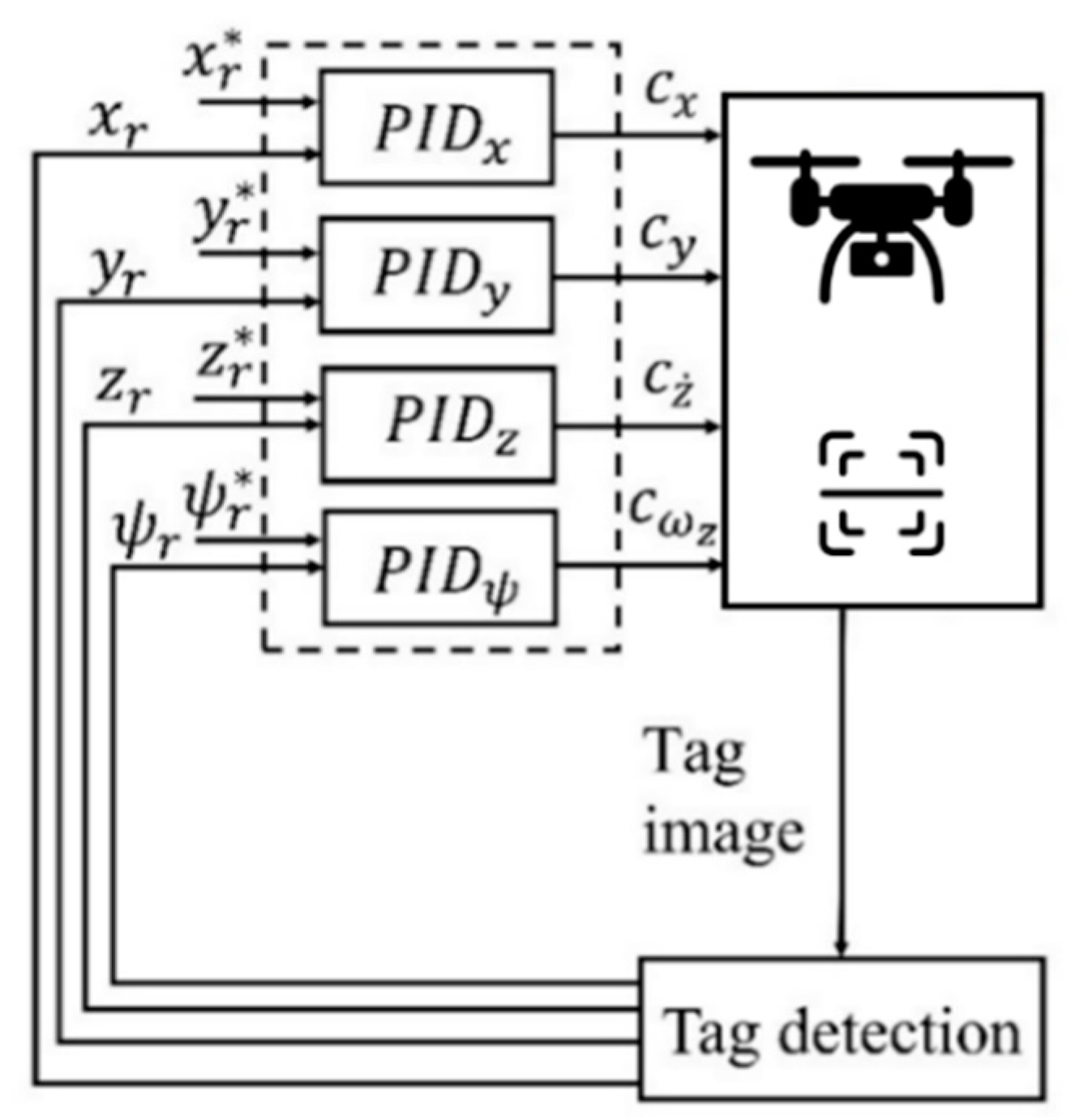
2.5. Experimental Design

The evaluation considered a target moving in a circular path in the plane. The experimental design as based on the parameters of the scenarios provided in Table 2. The radius of the circle was 1.5 m, and the speed of the target in each circle was 15 cm/s. The parameters used for the AMLQ-based autonomous landing are shown in Table 3.

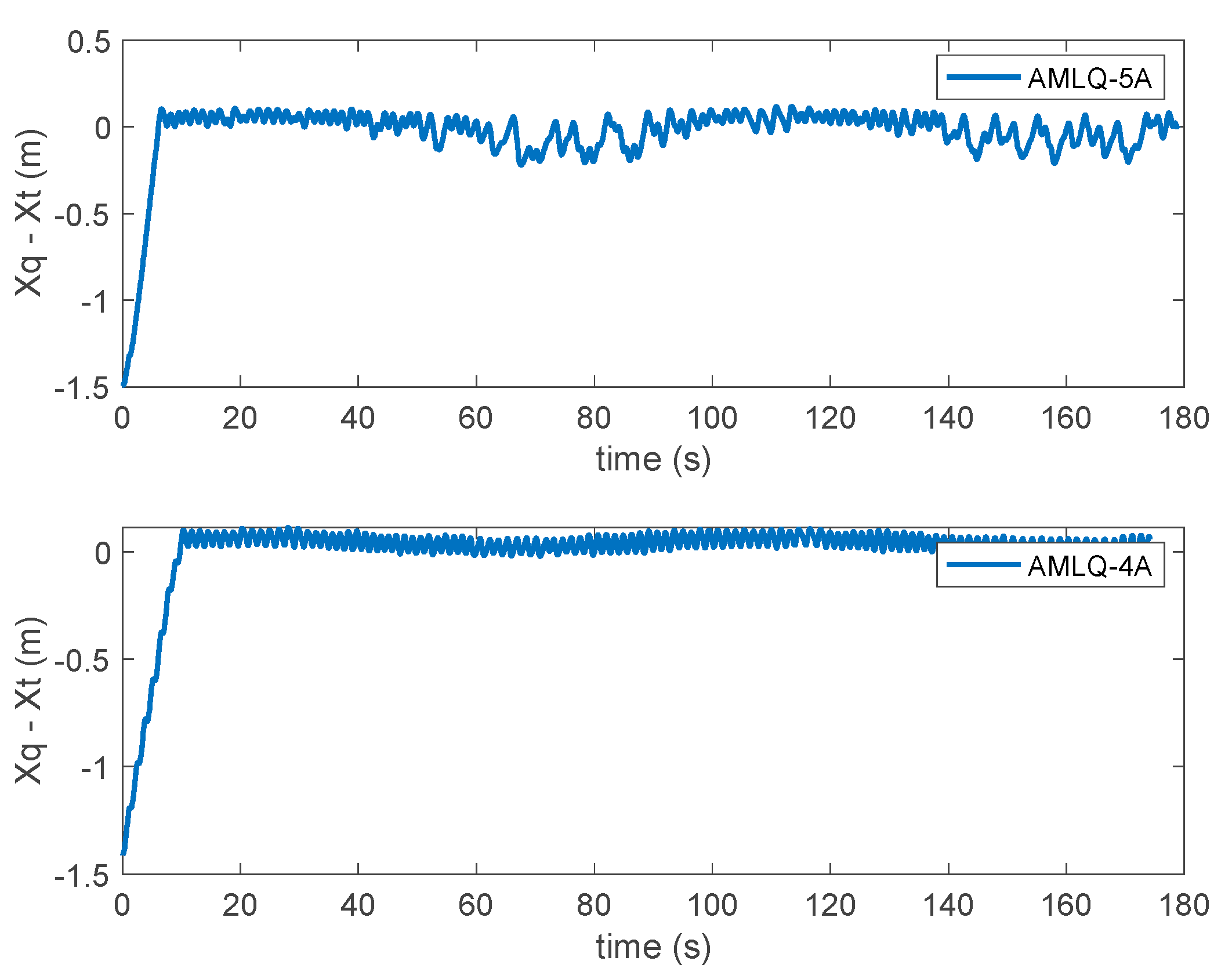
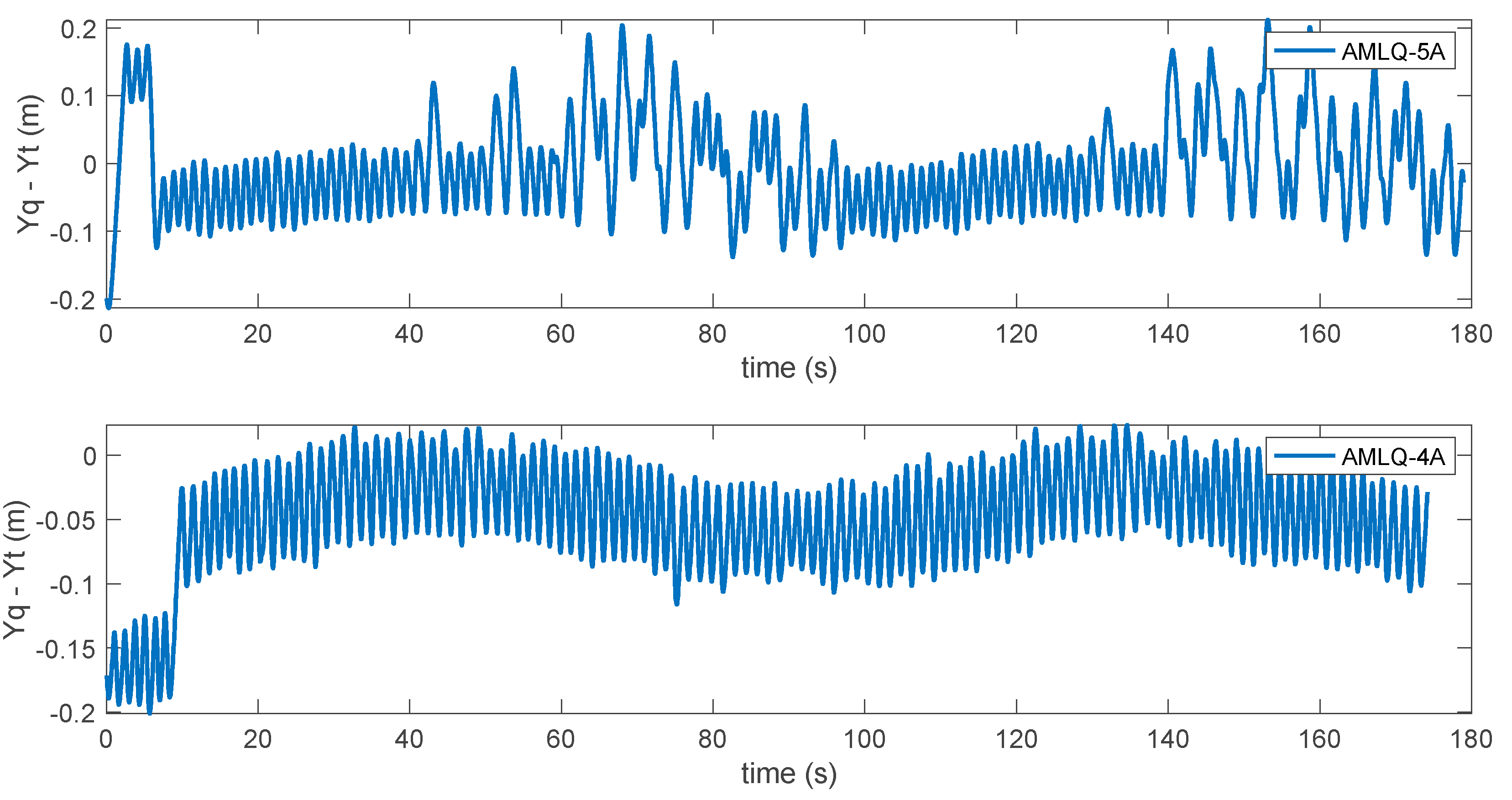
3. Results and Discussion

The evaluation results of the circular trajectory are presented in Figure 4. We used two types of the AMLQ model, the first one was with four actions, and we used the suffix 4A, the second one was with four actions, and we used the suffix 5A. The error with respect to X is presented in Figure 4. The figure shows that the AMLQ-4A model had a better performance and fewer errors than the AMLQ-5A model. This result can be explained by the less capable convergence of the five actions due to the bigger size of the latter. Similarly, we present the relative error with respect to Y-axis in Figure 5 for both the AMLQ-4A and AMLQ-5A models. It was also observed that the performance of the AMLQ-4A was better than the AMLQ-5A in terms of the magnitude of the error.
The performance of the developed AMLQ-4A and AMLQ-5A was compared with the PID control. The graphs of the relative error concerning X and Y are presented in Figure 6. It was observed that the magnitude of the error of the PID was higher than its equivalent of the AMLQ-4A and AMLQ-5A. However, the latter generated more oscillation compared with the PID. This result can be explained by the quantization of the actions in the QL. An approximating model of the Q-function via a neural network is recommended to solve this issue.
In addition to the error concerning X and Y, we present the conducted trajectory by the UAV and the target in Figure 7a–c for each of the AMLQ-5A, AMLQ4A, and PIDs. We observed that in both of the AMLQ models, the oscillation was higher for the ALMQ compared with the PIDs. However, the errors resulting from the AMLQ were fewer, as it was observed in the response graphs of the error on both X and Y. The main issue with the ALMQ was the low resolution of quantization which led to sudden actions of the UAV and more oscillation. On the other hand, increasing the resolution of the quantization led to a slow and even reduced convergence of the Q-matrix. In summary, we provided an RMSE for each of the three controllers: AMLQ-4A, AMLQ-5A, and PID, in Table 4. As is observed in Table 4, the lowest RMSE was scored by the AMLQ-5A.
The results reveal that the developed AMLQ can reduce the error of landing on the target. This issue is regarded as a valuable functionality that can be added to the UAV management software. Furthermore, it enhances human–UAV interaction and provides a safer condition for their collaboration.

4. Conclusions and Future Works

The problem of the autonomous landing of a UAV on a moving target is a nonlinear control problem with high dynamics. It includes tracking the target in the XY plane and landing on a moving target. To conduct the tracking, adaptive multi-level Q-learning was proposed. The definition of states considered quantizing the relative position between the UAV and the target in the X and Y coordinates. The definition of the action considered the quantization of the control signal in the X and Y plane using pre-defined quantization levels. One of the actions was proposed to be adaptive concerning the velocity to mitigate the problem of the low granularity of quantization which led to oscillation. The evaluation was conducted on various scenarios of trajectories of the moving target, namely linear and circular. For the evaluation, we provided the time response of the relative position of the UAV with respect to the target in the X and Y coordinates. The evaluation showed fewer resulted errors in the X and Y coordinates for the AMLQ model as compared with the PIDs-based tracking model. However, the lower levels of quantization resolution in the Q-matrix caused an oscillation performance when compared with the PIDs. Future work could involve the incorporation of a neural network to approximate the Q-function and to enable the handling of the continuous representation of states and actions, consequently obtaining smoother control and less oscillation.

Author Contributions

Conceptualization N.A.M., S.S.S. and R.O.; methodology, N.A.M., S.S.S., O.A., S.A.M., A.S. and R.O.; software, N.A.M., S.S.S., S.A.M., M.A.M. and N.A.-F.; validation, N.A.M., S.S.S., R.Q.M. and S.A.M.; formal analysis N.A.M., S.S.S., R.O. and N.A.-F.; investigation N.A.M., S.S.S., M.M.J. and S.A.M.; resources, N.A.M., S.S.S., O.A., A.S. and R.O. writing—original draft preparation, N.A.M., S.S.S. and S.A.M.; writing—review and editing, N.A.M., S.S.S., A.S. and S.A.M.; visualization and simulation N.A.M., M.M.J. and S.S.S.; supervision S.S.S., O.A., S.A.M. and R.O.; project administration, S.S.S., M.M.J., R.Q.M. and O.A., funding acquisition, S.S.S., O.A., R.O. and S.A.M. All authors have read and agreed to the published version of the manuscript.

Funding

This research was supported by the Zayed University cluster award R19046 and the Ministry of Higher Education (MoHE) through the Fundamental Research Grant Scheme (FRGS/1/2021/ICT01/UTHM/02/1) grant vot number K389. Communication of this research is made possible through monetary assistance by Universiti Tun Hussein Onn Malaysia and the UTHM Publisher’s Office via Publication Fund E15216.

Informed Consent Statement

Ethical review and approval are not applicable because this study does not involve humans or animals.

Data Availability Statement

Our data were auto-generated by the system during the training and simulation.

Acknowledgments

The authors would like to thank the College of Technological Innovation, Zayed University, Abu Dhabi, UAE, and Research Center for Unmanned Vehicles, Faculty of Mechanical and Manufacturing Engineering, Universiti Tun Hussein Onn Malaysia for supporting this work.

Conflicts of Interest

The authors declare that they have no conflict of interest to be addressed related to this work.

References

  1. Grippa, P.; Behrens, D.A.; Wall, F.; Bettstetter, C. Drone delivery systems: Job assignment and dimensioning. Auton. Robot. 2018, 43, 261–274. [Google Scholar] [CrossRef] [Green Version]
  2. Mishra, B.; Garg, D.; Narang, P.; Mishra, V. Drone-surveillance for search and rescue in natural disaster. Comput. Commun. 2020, 156, 1–10. [Google Scholar] [CrossRef]
  3. Mosali, N.A.; Shamsudin, S.S.; Alfandi, O.; Omar, R.; Al-fadhali, N. Twin Delayed Deep Deterministic Policy Gradient-Based Target Tracking for Unmanned Aerial Vehicle with Achievement Rewarding and Multistage Training. IEEE Access 2022, 10, 23545–23559. [Google Scholar] [CrossRef]
  4. You, H.E. Mission-driven autonomous perception and fusion based on UAV swarm. Chin. J. Aeronaut. 2020, 33, 2831–2834. [Google Scholar]
  5. Lygouras, E.; Santavas, N.; Taitzoglou, A.; Tarchanidis, K.; Mitropoulos, A.; Gasteratos, A. Unsupervised human detection with an embedded vision system on a fully autonomous uav for search and rescue operations. Sensors 2019, 19, 3542. [Google Scholar] [CrossRef] [PubMed] [Green Version]
  6. Joshi, G.; Pal, B.; Zafar, I.; Bharadwaj, S.; Biswas, S. Developing Intelligent Fire Alarm System and Need of UAV. In Proceedings of the International Conference on Unmanned Aerial System in Geomatics, Roorkee, India, 6–7 April 2019; pp. 403–414. [Google Scholar]
  7. Mostafa, S.A.; Mustapha, A.; Gunasekaran, S.S.; Ahmad, M.S.; Mohammed, M.A.; Parwekar, P.; Kadry, S. An agent architecture for autonomous UAV flight control in object classification and recognition missions. Soft Comput. 2021, 1–14. [Google Scholar] [CrossRef]
  8. Zhang, Y.; Yuan, X.; Li, W.; Chen, S. Automatic power line inspection using UAV images. Remote Sens. 2017, 9, 824. [Google Scholar] [CrossRef] [Green Version]
  9. Salvo, G.; Caruso, L.; Scordo, A.; Guido, G.; Vitale, A. Traffic data acquirement by unmanned aerial vehicle. Eur. J. Remote Sens. 2017, 50, 343–351. [Google Scholar] [CrossRef]
  10. Ke, R.; Li, Z.; Tang, J.; Pan, Z.; Wang, Y. Real-time traffic flow parameter estimation from UAV video based on ensemble classifier and optical flow. IEEE Trans. Intell. Transp. Syst. 2019, 20, 54–64. [Google Scholar] [CrossRef]
  11. Yahia, C.N.; Scott, S.E.; Boyles, S.D.; Claudel, C.G. Unmanned aerial vehicle path planning for traffic estimation and detection of non-recurrent congestion. Transp. Lett. 2021, 1, 1–14. [Google Scholar] [CrossRef]
  12. Bareiss, D.; Bourne, J.R.; Leang, K.K. On-board model-based automatic collision avoidance: Application in remotely-piloted unmanned aerial vehicles. Auton. Robot. 2017, 41, 1539–1554. [Google Scholar] [CrossRef]
  13. Aleotti, J.; Micconi, G.; Caselli, S.; Benassi, G.; Zambelli, N.; Bettelli, M.; Zappettini, A. Detection of nuclear sources by UAV teleoperation using a visuo-haptic augmented reality interface. Sensors 2017, 17, 2234. [Google Scholar] [CrossRef] [PubMed] [Green Version]
  14. Khadka, A.; Fick, B.; Afshar, A.; Tavakoli, M.; Baqersad, J. Non-contact vibration monitoring of rotating wind turbines using a semi-autonomous UAV. Mech. Syst. Signal. Process. 2019, 138, 106446. [Google Scholar] [CrossRef]
  15. Zhang, D.; Khurshid, R.P. Variable-Scaling Rate Control for Collision-Free Teleoperation of an Unmanned Aerial Vehicle. arXiv 2019, arXiv:1911.04466. [Google Scholar]
  16. Uryasheva, A.; Kulbeda, M.; Rodichenko, N.; Tsetserukou, D. DroneGraffiti: Autonomous multi-UAV spray painting. In Proceedings of the ACM SIGGRAPH 2019 Studio, Los Angeles, CA, USA, 28 July–1 August 2019; pp. 1–2. [Google Scholar]
  17. Beul, M.; Houben, S.; Nieuwenhuisen, M.; Behnke, S. Fast autonomous landing on a moving target at MBZIRC. In Proceedings of the 2017 European Conference on Mobile Robots (ECMR), Paris, France, 6–8 September 2017; pp. 1–6. [Google Scholar]
  18. Bähnemann, R.; Pantic, M.; Popović, M.; Schindler, D.; Tranzatto, M.; Kamel, M.; Grimm, M.; Widauer, J.; Siegwart, R.; Nieto, J. The ETH-MAV team in the MBZ international robotics challenge. J. Field Robot. 2019, 36, 78–103. [Google Scholar] [CrossRef]
  19. Lin, S.; Garratt, M.A.; Lambert, A.J. Monocular vision-based real-time target recognition and tracking for autonomously landing an UAV in a cluttered shipboard environment. Auton. Robot. 2017, 41, 881–901. [Google Scholar] [CrossRef]
  20. Fliess, M. Model-free control and intelligent PID controllers: Towards a possible trivialization of nonlinear control? IFAC Proc. Vol. 2009, 42, 1531–1550. [Google Scholar] [CrossRef] [Green Version]
  21. Sallab, A.E.; Abdou, M.; Perot, E.; Yogamani, S. Deep reinforcement learning framework for autonomous driving. IS&T Int. Electron. Imaging 2017, 29, 70–76. [Google Scholar]
  22. Kersandt, K. Deep Reinforcement Learning as Control Method for Autonomous Uavs. Master’s Thesis, Universitat Politècnica de Catalunya, Barcelona, Spain, 2018. [Google Scholar]
  23. Forster, C.; Faessler, M.; Fontana, F.; Werlberger, M.; Scaramuzza, D. Continuous on-board monocular-vision-based elevation mapping applied to autonomous landing of micro aerial vehicles. In Proceedings of the 2015 IEEE International Conference on Robotics and Automation (ICRA), Seattle, WA, USA, 26–30 May 2015; pp. 111–118. [Google Scholar]
  24. Sukkarieh, S.; Nebot, E.; Durrant-Whyte, H. A high integrity IMU/GPS navigation loop for autonomous land vehicle applications. IEEE Trans. Robot. Autom. 1999, 15, 572–578. [Google Scholar] [CrossRef] [Green Version]
  25. Baca, T.; Stepan, P.; Saska, M. Autonomous landing on a moving car with unmanned aerial vehicle. In Proceedings of the 2017 European Conference on Mobile Robots (ECMR), Paris, France, 6–8 September 2017; pp. 1–6. [Google Scholar]
  26. Gui, Y.; Guo, P.; Zhang, H.; Lei, Z.; Zhou, X.; Du, J.; Yu, Q. Airborne vision-based navigation method for UAV accuracy landing using infrared lamps. J. Intell. Robot. Syst. 2013, 72, 197–218. [Google Scholar] [CrossRef]
  27. Tang, D.; Hu, T.; Shen, L.; Zhang, D.; Kong, W.; Low, K.H. Ground stereo vision-based navigation for autonomous take-off and landing of uavs: A chan-vese model approach. Int. J. Adv. Robot. Syst. 2016, 13, 67. [Google Scholar] [CrossRef] [Green Version]
  28. Mostafa, S.A.; Mustapha, A.; Shamsudin, A.U.; Ahmad, A.; Ahmad, M.S.; Gunasekaran, S.S. A real-time autonomous flight navigation trajectory assessment for unmanned aerial vehicles. In Proceedings of the 2018 International Symposium on Agent, Multi-Agent Systems and Robotics (ISAMSR), Putrajaya, Malaysia, 27–28 August 2018; pp. 1–6. [Google Scholar]
  29. Falanga, D.; Zanchettin, A.; Simovic, A.; Delmerico, J.; Scaramuzza, D. Vision-based autonomous quadrotor landing on a moving platform. In Proceedings of the 15th IEEE International Symposium on Safety, Security and Rescue Robotics, Shanghai, China, 11–13 October 2017; pp. 200–207. [Google Scholar]
  30. Lee, D.; Ryan, T.; Kim, H.J. Autonomous landing of a VTOL UAV on a moving platform using image-based visual servoing. In Proceedings of the 2012 IEEE International Conference on Robotics and Automation, Saint Paul, MN, USA, 14–18 May 2012; pp. 971–976. [Google Scholar]
  31. Xu, Y.; Liu, Z.; Wang, X. Monocular Vision based Autonomous Landing of Quadrotor through Deep Reinforcement Learning. In Proceedings of the 2018 37th Chinese Control Conference (CCC), Wuhan, China, 25–27 July 2018; pp. 10014–10019. [Google Scholar]
  32. Lee, S.; Shim, T.; Kim, S.; Park, J.; Hong, K.; Bang, H. Vision-based autonomous landing of a multi-copter unmanned aerial vehicle using reinforcement learning. In Proceedings of the 2018 International Conference on Unmanned Aircraft Systems (ICUAS), Dallas, TX, USA, 12–15 June 2018; pp. 108–114. [Google Scholar]
  33. Araar, O.; Aouf, N.; Vitanov, I. Vision based autonomous landing of multirotor UAV on moving platform. J. Intell. Robot. Syst. 2016, 85, 369–384. [Google Scholar] [CrossRef]
  34. Polvara, R.; Sharma, S.; Wan, J.; Manning, A.; Sutton, R. Autonomous Vehicular Landings on the Deck of an Unmanned Surface Vehicle using Deep Reinforcement Learning. Robotica 2019, 37, 1867–1882. [Google Scholar] [CrossRef] [Green Version]
  35. Rodriguez-Ramos, A.; Sampedro, C.; Bavle, H.; De La Puente, P.; Campoy, P. A deep reinforcement learning strategy for UAV autonomous landing on a moving platform. J. Intell. Robot. Syst. 2019, 93, 351–366. [Google Scholar] [CrossRef]
  36. Polvara, R.; Patacchiola, M.; Hanheide, M.; Neumann, G. Sim-to-Real quadrotor landing via sequential deep Q-Networks and domain randomization. Robotics 2020, 9, 8. [Google Scholar] [CrossRef] [Green Version]
  37. Vankadari, M.B.; Das, K.; Shinde, C.; Kumar, S. A reinforcement learning approach for autonomous control and landing of a quadrotor. In Proceedings of the 2018 International Conference on Unmanned Aircraft Systems (ICUAS), Dallas, TX, USA, 12–15 June 2018; pp. 676–683. [Google Scholar]
  38. Srivastava, R.; Lima, R.; Das, K.; Maity, A. Least square policy iteration for ibvs based dynamic target tracking. In Proceedings of the 2019 International Conference on Unmanned Aircraft Systems (ICUAS), Atlanta, GA, USA, 11–14 June 2019; pp. 1089–1098. [Google Scholar]
  39. Ling, K. Precision Landing of a Quadrotor UAV on a Moving Target using Low-Cost Sensors. Master’s Thesis, University of Waterloo, Waterloo, ON, Canada, 2014. [Google Scholar]
  40. Malyuta, D.; Brommer, C.; Hentzen, D.; Stastny, T.; Siegwart, R.; Brockers, R. Long—Duration fully autonomous operation of rotorcraft unmanned aerial systems for remote—Sensing data acquisition. J. Field Robot. 2020, 37, 137–157. [Google Scholar] [CrossRef] [Green Version]
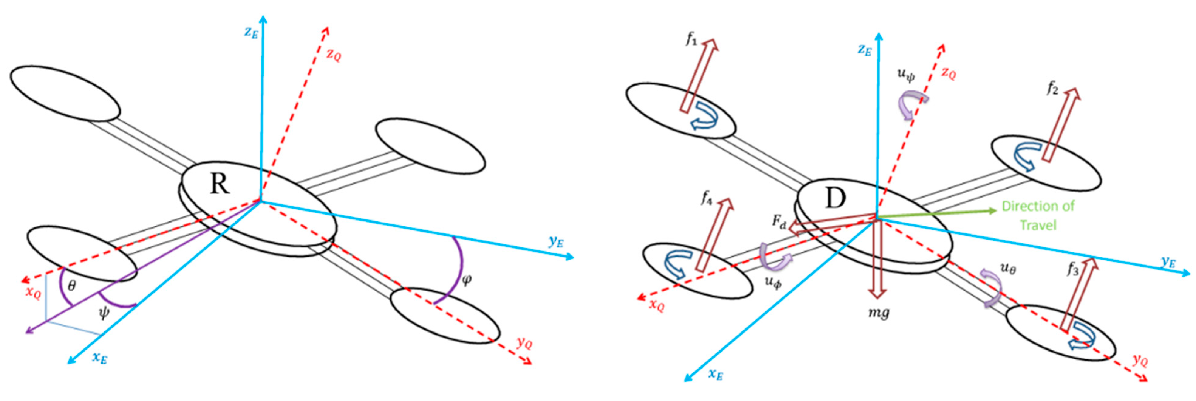
Figure 1. The classical structure of an autonomous landing control system.
Sustainability 14 08825 g001
Figure 2. The reference and the body frame of quadrotors [39].
Sustainability 14 08825 g002
Figure 3. The transformations for coordinating the frames [39].
Sustainability 14 08825 g003
Figure 4. The relative position of Y of the UAV with respect to the target for two variants of AMLQ: top AMLQ with five actions and bottom AMLQ with four actions. (the trajectory was circular at 1.5 m).
Sustainability 14 08825 g004
Figure 5. The relative position of X of the UAV with respect to the target for two variants of AMLQ: top AMLQ with five actions and bottom AMLQ with four actions (the trajectory was circular at 1.5 m).
Sustainability 14 08825 g005
Figure 6. The relative position of the UAV concerning the target based on PID control: top X coordinates and bottom Y coordinates (the trajectory was circular at 1.5 m).
Sustainability 14 08825 g006
Figure 7. The trajectory of the target and the tracking of the UAV for the preparation of the autonomous landing in (a) AMLQ-5A, (b) AMLQ-4A, and (c) PID. The orange lines represent the target movement trajectory.
Sustainability 14 08825 g007
Table 1. Symbols in the article and their interpretation.
SymbolMeaning
{ R } Reference frame
{ D } UAV frame
θ Pitch angle. This describes the orientation of the UAV with respect to Y R -axis of the reference frame
ϕ Roll angle. This describes the orientation of the UAV with respect to X R -axis of the reference frame
ψ Yaw angle. This describes the orientation of the UAV with respect to Z R -axis of the reference frame
g p The granularity level of position quantization
g v The granularity level of velocity quantization
( x d , y d , z d ) The position of the UAV
( v x d , v y d , v z d ) The velocity of the UAV
( x t a ,   y t a , z t a )The position of the target
e p = ( x d x t a , y d y t a ) The final error of the UAV with respect to the position
e v = ( v x d v x t a , v y d v y t a ) The final error of the UAV with respect to the velocity
p r e l The relative position of the UAV with respect to the target
v r e l The relative velocity of the UAV with respect to the target
N a The number of actions
s p , m a x The maximum value of the position in the state
s p , m i n The minimum value of the position in the state
s v , m a x The maximum value of velocity in the state
s v , m i n The minimum value of velocity in the state
d ϵ Decay factor of ϵ
1 , 2 Coefficients of the position and velocity rewarding term
3 , 4 , 5 , 6 Coefficients of the adaptive linear action model
7 , 8 , 9 , 10 Coefficients of the adaptive exponential action model
Table 2. PID gains used in the simulation.
PID Type P I D
x −1.0−0.05−0.005
y −1.0−0.05−0.005
z 0.80.10.1
ψ 0.80.10.1
Table 3. The parameters used for the AMLQ-based autonomous landing.
Parameter Name Parameter Value
α 0.8
γ 0.9
ϵ m a x 1.0
ϵ m i n 0.01
d ϵ 0.001
1 0.5
2 0.5
3 ,   5 4
4 , 6 0.032
7 , 8 ,   9 ,     10 0.25
Table 4. Summary of the steady error for each of the controllers.
CriterionAMLQ-4AAMLQ-5APID
RMSE8.96958.705210.0592
MSE80.452375.7811101.1883
Publisher’s Note: MDPI stays neutral with regard to jurisdictional claims in published maps and institutional affiliations.

