Article

A Calculation Model of Carbon Emissions Based on Multi-Scenario Simulation Analysis of Electricity Consumption

1
Management Science Research Institute, Guangdong Power Grid Corporation, Guangzhou 510062, China
2
School of Electric Power Engineering, South China University of Technology, Guangzhou 510641, China
3
Strategic Planning Department, Guangdong Power Grid Corporation, Guangzhou 510699, China
4
School of Accounting, Guangdong University of Foreign Studies, Guangzhou 510420, China
5
Guangzhou Power Supply Bureau, Guangdong Power Grid Corporation, Guangzhou 510630, China
*
Author to whom correspondence should be addressed.
Sustainability 2022, 14(14), 8765; https://doi.org/10.3390/su14148765
Submission received: 4 June 2022 / Revised: 10 July 2022 / Accepted: 15 July 2022 / Published: 18 July 2022

Abstract

:
In order to reach the peak of carbon emission in China by 2030 and to meet the low-carbon conversion of energy and the growing demand for electricity, this study aims to propose a more accurate and scientific method to calculate the carbon emissions of the entire power industry chain. This paper analyzes the historical actual operation data of the energy and power industry from 2000 to 2020, and originally proposes a carbon emission calculation model based on a multi-scenario simulation analysis of electricity consumption. This paper is an original study from the perspective of the whole industry chain of electricity production, transmission, and consumption. Firstly, a carbon emission model of the power system is established based on the carbon emission composition and transmission mechanism of the whole power industrial chain, which consists of calculation models for carbon emissions from overall electricity demand and carbon emissions from electricity network losses. Secondly, the concept of carbon emission coefficient is proposed, and the key parameters of the carbon emission coefficient of the power system are obtained through the econometric model. On this basis, the carbon emission coefficient is obtained by regression fitting of multiple key parameters according to historical data. Finally, electricity consumption per unit output value (ECPUOV) and per capita electricity consumption (PCEC) are used to predict electricity consumption in the next 15 years. This paper also makes a quantitative analysis of the relationship between CO 2 emissions from the power system and electricity consumption. This paper takes G province, which ranks first in total energy consumption and economic aggregate in China, as an example and calculates its CO 2 emissions and achievement of peak CO 2 emissions by multi-scenario analysis. The case study results show that the low carbon scenario(LC) is the best route for G province to peak CO 2 emissions from energy consumption. The method proposed in this paper can set an achievable goal of 2030 carbon peaking for the government and industry policymakers, and find a feasible implementation path.

1. Introduction

Being the world’s largest carbon emitter during the new era of global climate governance, China has been actively participating in the global response to climate change. In 2021, its carbon emission amounted to 11.9 billion tons, accounting for 33% of the world’s total carbon emission [1]. Therefore, China’s CO 2 emission reduction plays a vital role in the global carbon peak and carbon neutrality. China recently made major announcements concerning its more ambitious medium- and long-term climate goals. President Xi Jinping announced that China aims to have CO 2 emissions peak before 2030 and to achieve carbon neutrality before 2060 at the United Nations General Assembly in September 2020 [2].
The energy sector is the source of almost 90% of China’s greenhouse gas emissions, so energy policies must drive the transition to carbon neutrality [3]. Compared with developed countries in the world, China has not yet completed industrialization, and the growth of GDP still depends on the growth of energy consumption. Therefore, while China’s power industry has to reduce CO 2 emissions, it also needs to meet the increasing demand for electricity [4]. China accounted for nearly 30% of global electricity generation (7800TWh) in 2020, with its electricity production rising over 80%, or 6% annually, between 2010 and 2020. Despite the COVID-19 pandemic, the country saw a 3.7% annual increase in electricity generation in 2020 compared to 2019, and strong growth of 8% in 2021 to 8100 TWh [2]. The power generation sector in China emitted around 5.4 Gt of CO 2 , or around 47% of the country’s total energy sector emissions, in 2020. Power sector emissions increased by around 2% in 2020, despite the COVID-19 pandemic, and preliminary data point to a continued increase in 2021 [3]. Therefore, peak carbon emissions of the energy industry are an important prerequisite to this goal. According to the report of the IEA, in the carbon-neutral scenario, China’s final energy demand would gradually slow down and would begin to decline in around 2030, while the electricity demand would maintain continuous and rapid growth, with the total demand increasing by 60% in 2050 compared with that in 2020. Electricity would replace fossil energy to occupy a dominant position in final energy consumption [5]. McKinsey and Company estimated that power system emissions had the greatest reduction potential in China and plotted the global greenhouse gas abatement cost curve after 2030 [6]. Therefore, the process of carbon emission reduction within the power system determines the low-carbon development process directly.
In order to reach the peak of carbon emission in China by 2030 and to meet the low-carbon conversion of energy and the growing demand for electricity, this study aims to propose a more accurate and effective method to calculate the carbon emissions of the entire power industry chain, so as to quantitatively analyze the best path to achieve the carbon emission reduction goal. Previous studies on carbon emissions usually use the indirect factor influence method or the direct factor decomposition method. This paper proposes an innovative carbon emission calculation formula and the concept of electricity carbon emission factor based on the perspective of the whole electricity industry chain of energy production, transmission, and consumption. This method considers both direct factors such as installed fossil energy and electricity that affect carbon emissions, and indirect factors such as GDP and population, and makes full use of actual operational energy data to predict regional carbon emission trends and peak situations, and realize the evaluation of carbon emission and change trend of energy and power consumption in multiple scenarios.
As the largest economic province in China, G province’s green and low-carbon transformation is arduous because its energy and electricity demand increases year by year. During the 13th Five-year Plan period, G province’s GDP increased by 6% annually. In 2020, G province’s total energy consumption reached 345 million tons of standard coal. Its electricity demand increased from 406 billion kWh in 2010 to 786.7 billion kWh in 2020, ranking top in China. This paper takes G province’s actual operation data as an example to calculate carbon emissions. Therefore, it can provide an important reference for typical regions like G province to promote energy consumption transformation, formulate energy construction plans and other strategic energy transformation measures, reduce carbon emissions, and control global temperature rise. Considering the strategic goals of carbon peak in 2030 and carbon neutralization in 2060 proposed by China, this paper selects the present to 2030 as the main research period and extends to 2035 to observe the downward trend of carbon emissions. In addition, whether G Province, a large energy-consuming Province, can reach its peak in 2030 is of typical and important significance for China as a whole. Therefore, this paper takes the actual operation data of G Province as an example to calculate carbon emission reduction, which plays an important demonstration and reference role in formulating energy construction planning and other energy transformation strategic measures and controlling global temperature rise. Furthermore, it proves that the model proposed in this paper can provide scientific references for regional power systems to accurately estimate the achievement of peak carbon emissions and to design policies and paths for peak carbon emissions.

2. Literature Review

According to the studies of carbon emission, its calculation methods can be divided into those based on indirect variables and those based on direct variables.

2.1. Carbon Emission Calculation Methods Based on Indirect Variables

These methods mainly use indirect variables, which have indirect effects on carbon emissions at a macro level, to calculate carbon emissions. In other words, key indirect variables, such as GDP, population, and other factors, are selected to analyze their quantitative relationship with carbon emissions and predict the peak of CO 2 emissions. The main methods include the Kaya identity [7], the STIRPAT model [8], the environment Kuznets curve (EKC) [9], the LMDI model [10,11], etc. Fan et al. (2020) studied influencing factors and countermeasures of industrial carbon emissions in Hebei Province based on the Kaya model [7]. The Kaya identity focuses on the relationship between economic factors and carbon emission, and predicts the time to peak carbon emissions. However, carbon emission is influenced by many factors, it is not accurate to predict the time to peak carbon emissions only based on one single type of factor. Compared with the Kaya model, the STIRPAT model is more accurate as multiple parameters are used according to the actual changes of the evaluated object and the scope of calculation. Kaya and STIRPAT models are evaluated so that the latter could get more accurate analysis results [12]. The STIRPAT model is used to analyze the influencing factors and the time to peak carbon emissions in Guangdong by incorporating the service level and the degree of trade openness into the model based on Guangdong’s development [13]. However, using the LMDI model to analyze the main driving factors of carbon emissions can be found that it requires less data and has a wide application range. Wang et al. (2017) used the LMDI method to divide CO 2 emissions into those from the population, economic output, industrial structure, capacity intensity, and energy structure, and analyzed the contribution of different driving factors at national and provincial levels [14]. These methods only require macroeconomic data. Therefore, they have low data requirements and are easy to calculate. However, these indirect calculation methods only consider apparent CO 2 consumption rather than actual CO 2 consumption. In addition, as comprehensive parameters are applied, plus various losses and errors, the results may not be accurate, but can generally be used as the verification basis for the results calculated by other methods [15].

2.2. Carbon Emission Calculation Methods Based on Direct Variables

These methods mainly use direct influencing factors from resource utilization to construct carbon emission calculation models. They use direct influencing factors, including energy production, consumption, and demand, to conduct modeling in the whole process. Common methods include IPCC default method [16], regression method, system dynamics method, scenario analysis method, etc. In [17], the IPCC default method is used to evaluate CO 2 emissions from energy consumption in Guangdong Province. Peter et al. (2016) used the IPCC default method at different levels to calculate the carbon footprint of agricultural products [18]. The lower-level IPCC default method is usually used to roughly estimate emissions for it is simple and easy to operate. However, it fails to consider the resource of different regions to ensure the accuracy of carbon emissions calculation. The higher-level IPCC default method is generally considered to be too complex to be feasible. The remaining methods require screening of variables, and the selection of independent variables can be obtained by covariance and Granger test analysis [19,20], and the ARDL method can further investigate the long-run and short-run relationships between the independent and dependent variables [21,22,23,24,25]. The regression method is widely used due to its ease of calculation and the need for fewer variables. For example, Zhou et al. (2021) analyzed the relationship between the expansion of urban construction land and carbon emissions by constructing carbon emission calculation models and VAR models based on Nanchang’s time series data from 1995 to 2017 [26]. Compared with the regression-based models, the models based on system dynamics take the interaction between variables into consideration and are more accurate. Ma et al. (2019) predicted Shandong’s carbon emissions from 2017 to 2030 through a system dynamics-based model under four design schemes [27]. Although these methods fully consider the influence of variables, their models are relatively large and their calculation is complex. The interaction between variables needs to be set in advance. The quality of their models depends on whether preconditions are set accurately [28]. The scenario analysis-based method can fully use current economic and energy policies and build a carbon emission calculation model based on direct influencing factors involved in resource endowments and the whole process, including energy production, consumption, and demand. Therefore, it is more accurate and it can be combined with the above methods [29,30]. For example, ZHANG et al. (2021) combined the LMDI model and scenario analysis, firstly decomposed China’s carbon emissions exponentially, identified influencing factors, and then conducted scenario analysis on carbon intensity targets in 2020 and 2030, thus helping policy-makers evaluate the effectiveness of current policies in detail [31].
In general, the above studies have explored China’s carbon emission reduction potential and its contributing factors in the future. Still, few studies have been conducted on the carbon emission of electricity consumption from the perspective of the whole industrial chain, including electricity production, transmission, and consumption. The carbon emission measurement method based on power consumption proposed in this paper combines econometric with scenario analysis. This method comprehensively considers the direct factors such as fossil energy installation and electricity that affect carbon emissions, as well as indirect factors such as GDP and population, and makes full use of the actual operating energy data to build a carbon emission model to improve the accuracy of carbon emission measurement and uses the utilization rate of the installed capacity of fossil power generation (URICFPG), the proportion of fossil power generation (PFPG), the conversion rate of fossil power generation (CRFPG), and the grid loss rate as variables to construct an emission factor model of unit electricity. It also uses historical data from the last ten years to determine the model factor. This paper uses the model to predict G province’s carbon emissions, a typical economic and energy-consuming province, under three different energy construction scenarios, namely the reference scenario (REF) the low carbon scenario (LC), and the security constraint scenario (SC). The calculation model comprehensively considers direct factors, such as the installed capacity and power generation of fossil energy, and indirect factors, such as the GDP and population, that affect carbon emissions. A carbon emission model constructed with actual energy data improves the accuracy of carbon emission calculation. This paper hypothesizes electricity consumption scenarios in a typical region in China and studies the achievement of peak carbon emissions in different hypothetical scenarios, hoping to provide a research basis for the formulation of carbon emission reduction policies and measures.

3. Calculation Model and Scenario Design

3.1. Calculation Model of Carbon Emissions

3.1.1. Total Carbon Emission Model

Carbon emissions from the electric power system include carbon emissions from the electricity generation side and network losses. Their carbon emission composition and transmission mechanism are shown in Figure 1.
Therefore, the carbon emission model of power system can be composed of two parts of carbon emissions calculation: the one generated by the electricity generated to meet the overall electricity demand (OED) in the region; the other one generated by the network loss of grid. The specific formula is as follows:
T c t = S c t + P c t
where t represents time; T c t , the carbon emissions of power system in the year t; S c t , carbon emissions from electricity generation to meet the overall electricity demand (OED) in the year t; P c t , carbon emissions from grid losses in the year t.

3.1.2. Carbon Emissions from Electricity Generation to Meet Overall Electricity Demand

The formula for carbon emissions from society-wide electricity consumption is as follows:
S c t = ( E t + E 1 t E 2 t ) × α t
where S c t represents carbon emissions from electricity generation in the region to meet the overall electricity demand (OED) in the year t; E t , the overall electricity demand (OED) in the region in the year t; E 1 t , electricity that the region delivers to another region; E 2 t , electricity that the region receives from another region. According to inter-province long-term agreements, both E 1 t and E 2 t are constants, and α t represents the carbon emission factor of electricity in the region in the year t.
  • Overall Electricity Demand E t :
    The overall electricity demand (OED) is a key parameter in predicting carbon emissions. The electricity consumption per unit output value (ECPUOV) method [32] can be used to predict industrial electricity consumption, and PCEC can be used to predict residential electricity consumption. ECPUOV statistically analyzes the ECPUOV of the three major industries (agriculture, industry, and service sector) and determines the ECPUOV of the three industries according to economic development and industrial structure adjustment. Plus annual residential electricity consumption, it predicts the overall electricity demand (OED) in a designated area [33]. The formula is as follows:
    E t = G t i Q t i + P t K t
    where E t represents total electricity consumption in the year t; G t i , the output value of unit consumption of the industry i in the year t; Q t i , the output value of the industry i in the year t; P t , the total population in the region in the year t; K t , per capita residential electricity consumption in the year t.
  • Carbon Emission Factor α t :
    According to the results of the Pearson correlation coefficient analysis in Appendix A, and combined with the experience of industry experts and the studies of [34,35,36,37,38,39], this paper defines the carbon emission factor α t as a parameter that describes the association of the total carbon emissions in the region with the URICFPG, the PFPG and the CRFPG. The calculation formula of the carbon emission factor is as follows:
    α t = α 0 + α 1 A t + α 2 Q t + α 3 η t + ε t
    where α t (explained variable) represents the carbon emission factor in the year t; A t (key explanatory variable), the URICFPG in the year t; Q t , the PFPG in the year t; η t , the CRFPG in the year t. ε t is an error, and α 0 , α 1 , and α 2 are variation coefficients.
    In order to avoid pseudo regression of data, the sequence of each variable must be stable in the regression analysis of explanatory variables and explained variables. This paper uses Eviews to establish an econometric model for the ADF unit root test and cointegration analysis. See Appendix A for specific analysis and results. Firstly, the stationarity of each variable sequence is determined according to the results of the ADF test, and the nonstationary sequence is transformed into a stationary sequence by difference. The test results show that the carbon emission coefficient and its strongly related factors, such as A t , Q t and η t , are stable after the first-order difference (FOD). Therefore, the Johansen cointegration test can be performed between these four variables. The results of the cointegration test show that there is at least one cointegration relationship among the four variables at the 5% confidence level, so regression analysis can still be carried out even in the case of non-stationary series.

3.1.3. Carbon Emissions from Electricity Network Losses

Carbon emissions from electricity network losses mainly come from electricity transmission losses. We can get a carbon emission curve by calculating electricity losses in electricity transmission and the carbon emission factor of electricity in the region.
P c t = W t × ϕ t × α t
where P c t represents carbon emissions from network losses in the region; W t , the power supply in the region in the year t; ϕ t , the grid loss rate in the year t; α t , the carbon emission factor of the region in the year t. The main influencing factors of network loss rate include technical factors, such as load characteristics and grid structure, and management factors, such as misplaced electricity and anti-electricity stealing management. Considering both technical and management factors, the grid loss rate ϕ t has a very limited range of variation, so it is treated as a constant according to actual statistical data.

3.2. Design of Multi-Scenario

To comprehensively explore possible approaches to control global greenhouse gas in the future, this paper designs the reference scenario (REF), the low carbon scenario (LC), and the security constraint scenario (SC) based on the development of various types of renewable energy within the range of resource endowments. The above model is used to analyze carbon emissions in these three scenarios and to predict carbon emissions and the time to peak carbon emissions from the perspective of electricity.
  • REF: No climate change measures are adopted. The technology, installed structure, and structure of power generation remain at the same level as that in the year 2021, and the final electricity demand consistent with this emission scenario is met. Coal power has basically realized clean development. The coal consumption rate of generation has a limited reduction space for the generation has basically realized clean development. coal power and new energy power are developing at a low rate. The installed capacity and power generation of thermal power always dominate. According to the current power supply structure, by 2030, the installed capacity of fossil power will account for 61.8%, and electricity generated from fossil energy will account for 64%. Grid losses remain at the current level.
  • LC: The latest industrial planning, clean energy goals, and low carbon policies stipulated by the 14th Five-year Plan of G Province have been realized. Coal power gradually decreases after slow growth. New energy power generation develops at a moderate speed. Technical and management measures for reducing grid losses develop at a moderate speed. By 2030, the percentages of the installed capacity of fossil power and power generated from fossil power are expected to fall to 48.7% and 50.4% respectively.
  • SC: This scenario considers constraint factors such as rapid growth of electricity consumption and shortages of gas and water based on the low carbon scenario. China’s electricity consumption will grow rapidly and reach 920 billion kWh in 2025, 1050 billion kWh in 2030, and 1130 billion kWh in 2035. There will be a natural gas shortage, and the rise in natural gas prices will lead to an increase in electricity costs. Thus, annual power generation utilization hours are expected to experience a significant decrease. Moreover, the gap in the power supply from western China will widen. It is estimated that 190 billion kWh of electricity will be sent from western China to eastern China during the 14th Five-year Plan period. Under the above security constraints, coal power will compensate for the electricity gap to achieve electricity balance. On the power supply side, the installed capacity of non-fossil energy and power generated by non-fossil energy will gradually play a dominant role after 2025. By 2030, the percentages of the installed capacity of fossil and power generated from fossil energy are expected to drop to 48.7% and 54.6% respectively. On the electric grid side, the electric grid loss reduction level will be constantly optimized. The electric grid loss rate will be reduced to 3.75% beyond expectations and remain relatively stable.

3.3. Data Source

  • Source of data for calculating the carbon emission factor. The data of A t used in the REF are from the Brief Introduction to the Operation of Electric Power Industry of China Electricity Council. The data of Q t and η t used in the REF are calculated based on electricity generated from different types of energy and unit standard coal consumption specified in the China Energy Statistical Yearbook. The data of A t , Q t , η t , and electricity transmitted according to the West-to-East Power Transmission Project used in the LC and the SC are estimated according to the 14th Five-year Plan for Energy Development of G Province.
  • Historical output values and ECPUOV of the three major industries of the national economy used to predict electricity consumption are from the G Province Statistical Yearbook. The output values of the three major industries, unit electricity consumption, and per capita household electricity consumption (PCHEC), which are used in the REF, the LC, and the SC, are all reasonably estimated based on historical data.
  • The data of grid loss rate of G province power system used in the REF are from the Energy Statistics of G Province Electricity Trade Association, and the data used in the LC and the SC are reasonably estimated according to the 14th Five-year Plan for Energy Development of G Province.

4. Estimated Carbon Emissions of G Province Power System Based on Designed Scenarios

4.1. Calculation of Key Parameters of the Model

4.1.1. Calculation of Carbon Emission Coefficient

Based on the multiple regression model (4), using the historical data from 2010 to 2020, the evenness test of variables and the correlation analysis of multivariable are carried out by using Eviews software, and the strong correlation between their variables and dependent variables is verified according to the Pearson coefficient. Further using R software, based on the least square method (OLS), multiple linear regression analysis was carried out, and the goodness of fit was 0.967. After determining the variable coefficients of the emission coefficient model, the calculation model (6) is obtained, which shows that the increase in the installed utilization rate of fossil energy and the proportion of fossil energy electricity will increase the carbon emission coefficient, and the increase in the conversion rate of fossil energy will reduce the carbon emission coefficient. The model test results obtained through fitting calculation are shown in Table 1 below (please see the Appendix A for detailed calculation):
The carbon emission factor after fitting is calculated as follows:
α t = 0.4765 + 0.1703 A t + 0.5747 Q t 1.2024 η t
Carbon emission factors for the next 15 years are estimated based on Formula (6), as shown in Table 2 below.

4.1.2. Power Consumption Prediction of the Whole Society

According to the comprehensive analysis of the development of various industries in G Province, it is estimated that in 2025, 2030, and 2035, the unit consumption of the output value of the primary industry will be 0.033 kwh/CNY, 0.034 kwh/CNY, and 0.035 kwh/CNY respectively; the unit consumption of output value of the secondary industry is 0.103 kwh/CNY, 0.090 kwh/CNY, and 0.078 kwh/CNY respectively; the unit consumption of output value of the tertiary industry is 0.025 kwh/CNY, 0.022 kwh/CNY, and 0.018 kwh/CNY respectively; the per capita residential electricity consumption is 1200 kwh/person, 1400 kwh/person, and 1600 kwh/person respectively. Using the output value unit consumption method to predict the industrial power consumption, and using the per capita power consumption method to calculate the residential power consumption, the prediction results of the whole social power consumption in G Province are shown in Table 3 below (please see Appendix B for detailed calculation):

4.1.3. Grid Loss Rate

The 14th Five-year Plan for Energy Development of G Province estimates that grid losses may develop at high, medium, and low rates, as shown in Table 4. As for high grid losses, grid losses will maintain the current level (REF). As for medium grid losses, certain management and technical measures will be taken to improve and realize the target value stipulated by the 14th Five-year Plan (LC) and G province’s grid loss rate will be reduced to 3.8% in 2025. As for low grid losses, after the grid loss rate is reduced to 3.8% at the end of the 14th Five-year Plan, it will become more difficult to reduce grid losses. It can be slightly reduced by the demand-side response and other technical measures, and will be reduced to 3.75% in 2030.

4.2. Quantitative Evaluation Analysis in Different Scenarios

4.2.1. Reference Scenario

  • Estimated Carbon Emissions
    Carbon emissions in the REF are shown in Table 5 below.
  • Carbon Emission Curve
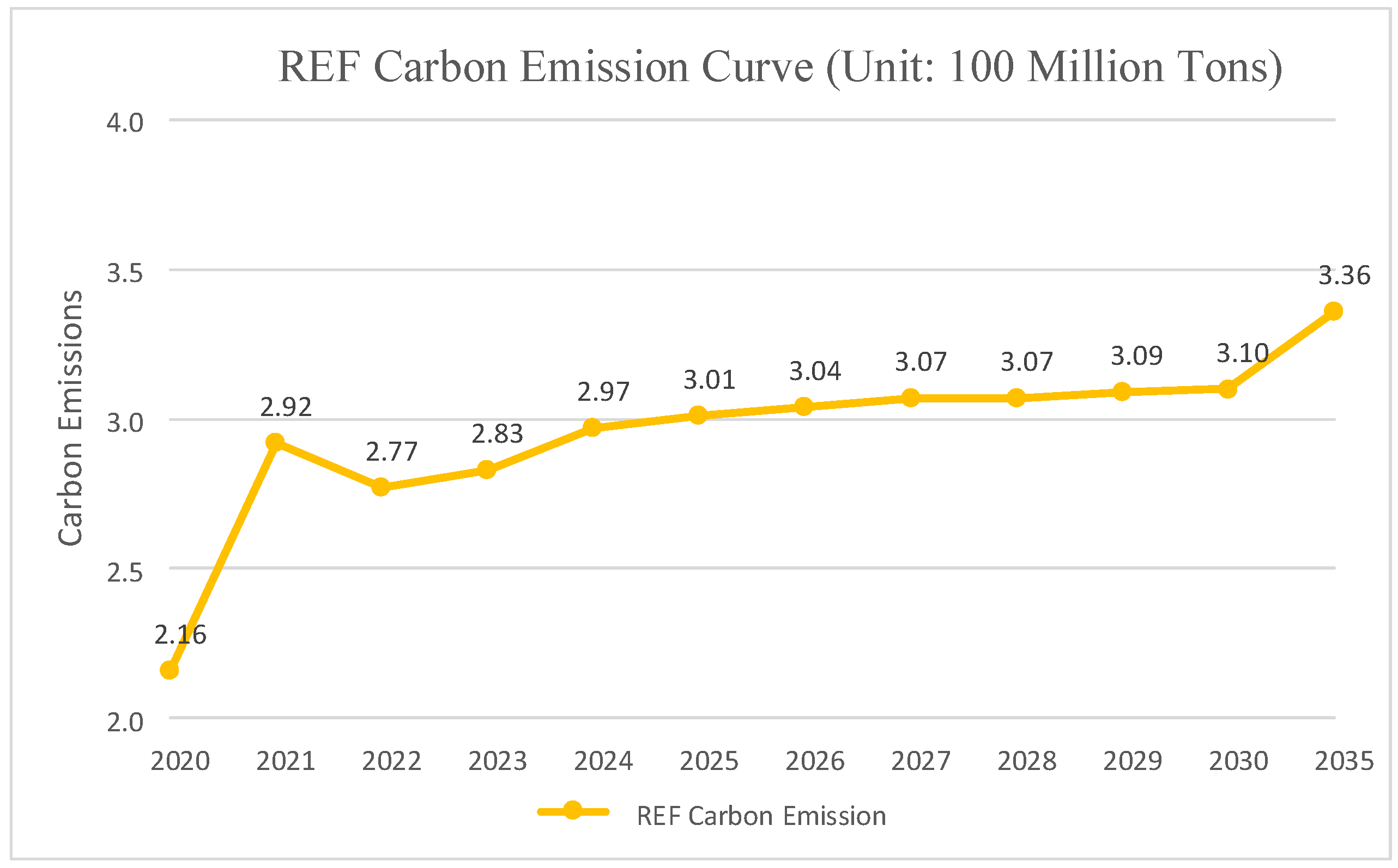
    In the REF, the carbon emission curve of G province’s power system is shown in Figure 2 below. The carbon emissions will gradually increase before 2030, but they will not peak. In 2030, the carbon emissions will stand at 310 million tons, of which 294 million tons are from total electricity consumption and 16 million tons are from grid losses.

4.2.2. Low Carbon Scenario

  • Estimated Carbon Emissions
    According to calculation results of the carbon emission factor model and the carbon emission model for the overall electricity demand (OED), estimated carbon emissions under the LC are shown in Table 6 below.
  • Carbon Emission Curve
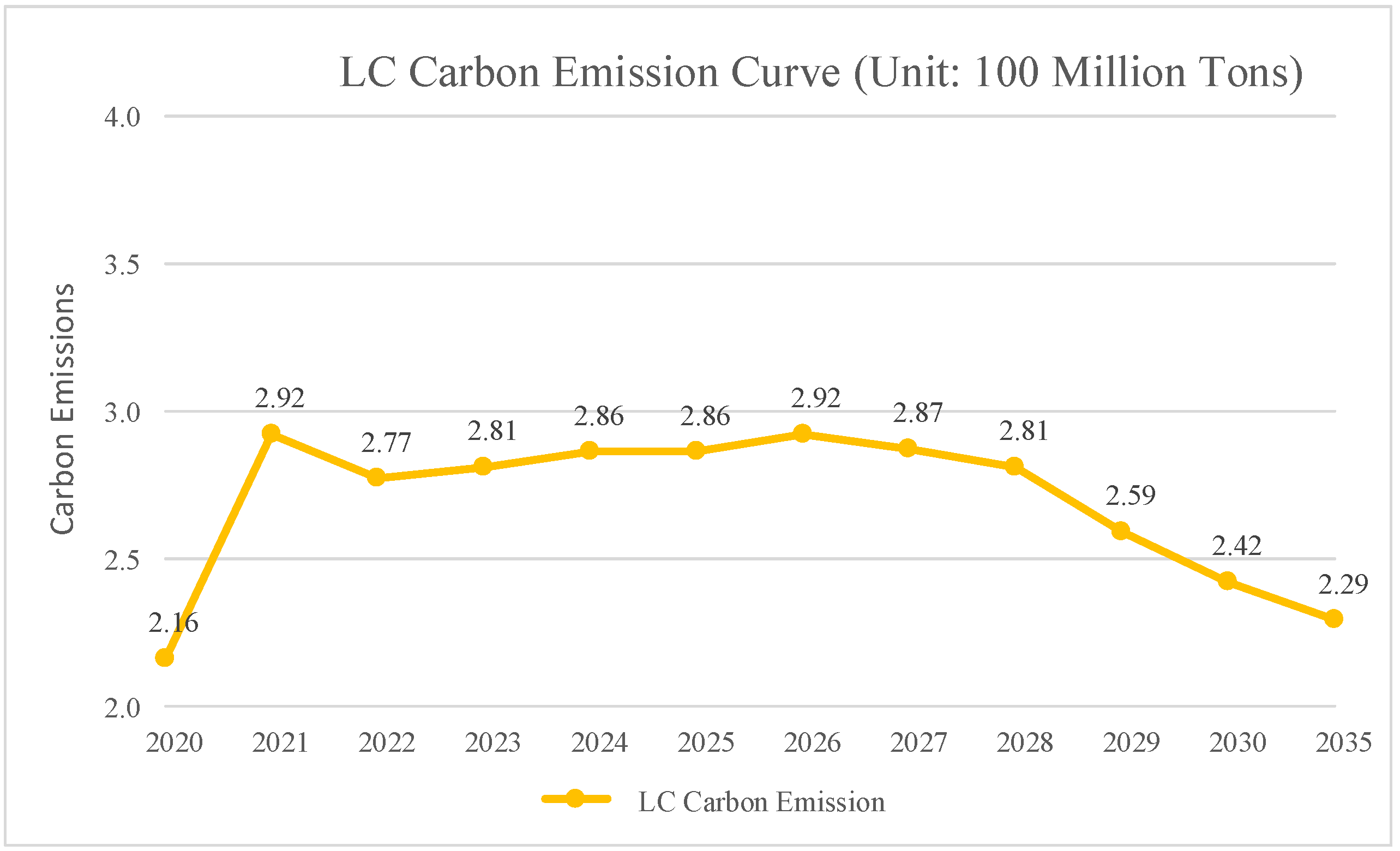
    In the LC, the carbon emission curve of G province’s power system is shown in Figure 3 below. In around 2026, G province will peak carbon emissions. In 2030, G province’s power system carbon emissions will stand at 242 million tons, of which 230 million tons are from total electricity consumption and 12 million tons are from grid losses.

4.2.3. Security Constraint Scenario

  • Estimated Carbon Emissions
    Based on the hypothesized electric quantity and power supply structure in the security constraint scenario, estimated carbon emissions in the SC are shown in Table 7.
  • Carbon Emission Curve
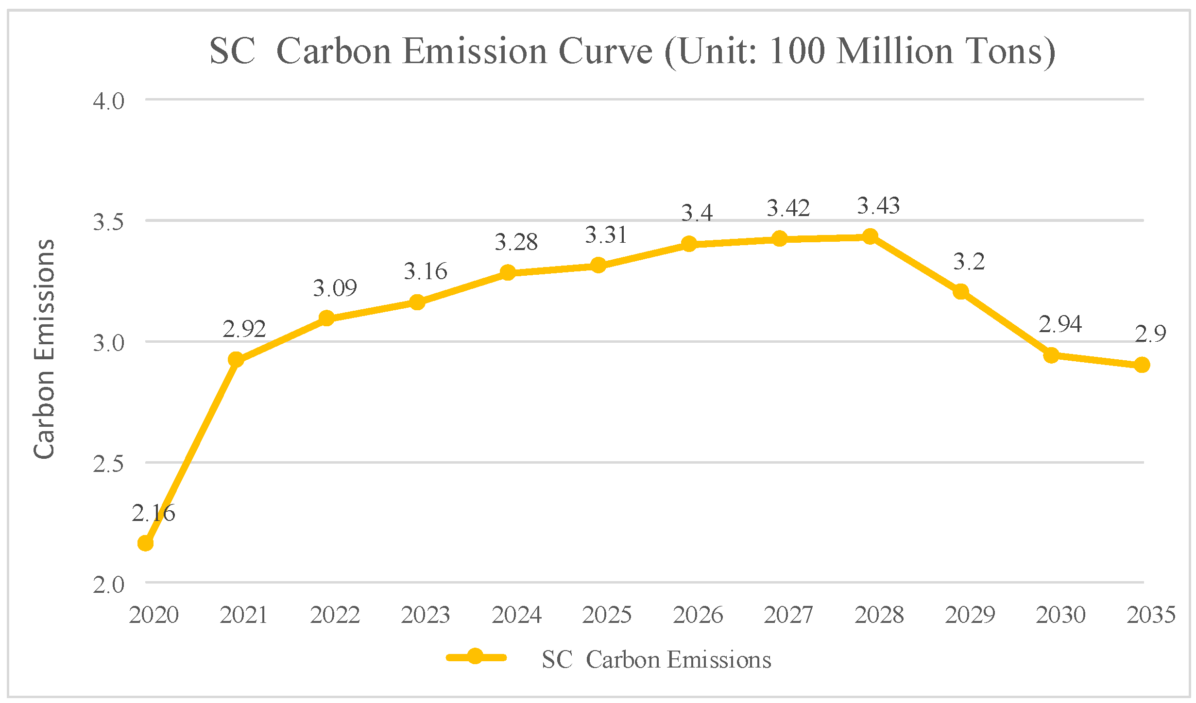
    In the SC, the carbon emission curve of G province’s power system is shown in Figure 4 below. carbon emissions from electricity consumption in G province will reach peak carbon emissions in around 2028. In 2025, carbon emissions from electricity consumption in G province will amount to 330 million tons, and in 2030, 294 million tons.

4.2.4. Summary and Discussion of Three Scenarios

To sum up, on the premise of no influence on economic and population growth. In the REF, G province’s power system will not achieve peak carbon emissions before 2030; in the LC, G province’s power system will peak carbon emissions in around 2026; in the SC, it will peak carbon emissions in 2028. The REF cannot meet China’s overall strategic deployment for peak carbon emissions by 2030. The SC can meet the target of peak carbon emissions by 2030, but the overall progress is a little slow. Therefore, it should be used as a special countermeasure in extreme climates. The LC can meet the target of peak carbon emissions and features a more positive climate strategy. Moreover, it is designed based on the 14th Five-year Plan for Energy Development. It fully considers the development potential of new energy and the planning and construction of electric grid supply and consumption facilities. Therefore, it can make up for volatility, randomness, and intermittent in new energy power generation. It is safer and more stable. So it is the best solution for regular operation.
In the three scenarios designed by this paper (the REF, the LC, and the SC), according to the resource endowment of G Province, change the values of different influencing factors, and calculate the time of carbon peak in G Province. The study of this paper shows that economic development and population growth are the key driving factors for CO 2 emissions from the power sector. URICFPG, PFPG, and CRFPG are the most important restraining factors in the CO 2 emission growth of the power system.

5. Discussion

The quantitative carbon emission calculation model proposed in this paper effectively estimates the carbon emissions and the peak time of G province’s power carbon emissions in three energy scenarios. The calculation model comprehensively takes the direct and indirect influencing factors into account, such as the actual operating parameters of the whole power chain and national economic parameters, and so on. Compared with Yuan Tao et al. [9], both consider the influence of renewable energy on the power sector’s peaking carbon emissions. Yuan Tao et al. constructed a bottom-up carbon emission reduction model for the power sector based on resource utilization, while this paper comprehensively considers the influence of the economy, population, and other factors on total electricity consumption. The study of Yuan Tao et al. proves that based on control policies against the background of low-level macroeconomic development and medium technical development, total carbon emissions of the power sector will peak by 2030, in which case, carbon emission reduction costs stand at the lowest. Based on their study, this paper conducts in-depth research on a typical region with relatively high energy consumption intensity in China, and analyzes whether a province with high economic development and energy consumption can peak carbon emissions before 2030. The conclusion shows that a province with large energy consumption can also peak carbon emissions before 2030, which is consistent with the overall trend in the power sector studied by Yuan Tao et al., and further proves that China can comprehensively achieve peak carbon emissions by 2030. Compared with the study on G province’s peak carbon emissions by Ping et al. [14], both Ping and this paper take into account factors such as the population and GDP. Ping incorporates the service level and the degree of trade openness into the calculation model. In contrast, this paper includes the URICFPG and the PFPG in the calculation model. Both studies agree that G province can reach peak carbon emissions by 2030.

6. Conclusions

This paper originally proposes a carbon emission calculation model based on a multi-scenario simulation analysis of electricity consumption. It constructs G province’s carbon emission model based on the perspective of the whole power system chain, accurately fits the carbon emission factor, and quantitatively estimates the carbon emissions and the peak time in the REF, the LC, and the SC situation. The calculation model comprehensively takes into account the direct influencing factors such as the actual operating parameters of the whole power chain and the indirect influencing factors such as the national economic parameters. This model makes up for the shortcomings of used calculation models which only consider indirect factors such as the population, technology, and economy. It is more scientific and accurate to calculate carbon emissions and the peak of carbon emissions. The model proposed in this paper has a positive reference value for the study of carbon emissions in different industries and regions. It has practical value for the future assignment of regional carbon emission responsibility and the establishment of a corresponding assignment system.

Author Contributions

Conceptualization, X.C. and Z.L.; methodology, Q.L.; software, G.Z.; validation, X.C. and G.Z.; formal analysis, P.L.; data curation, K.Y.; investigation, P.L.; writing—original draft preparation, X.C.; writing—review and editing, Z.L.; supervision, Z.G.; project administration, Z.G. All authors have read and agreed to the published version of the manuscript.

Funding

Xiaoli Chen was financially supported by the Key innovation Projects of China Southern Power Grid (GDKJXM20212083). Qian Li was financially supported by the Key Program of the National Social Science Fund of China (20AZD092).

Institutional Review Board Statement

Not applicable.

Informed Consent Statement

Not applicable.

Data Availability Statement

The calculation data used in this paper have been explained in Section 3.3.

Conflicts of Interest

The authors declare no conflict of interest.

Abbreviations

The following abbreviations are used in this manuscript:
EKCEnvironment Kuznets Curve
OEDOverall Electricity Demand
PCECPer Capita Electricity Consumption
PCHECPer Capita Household Electricity Consumption
URICFPGUtilization Rate of the Installed Capacity of Fossil Power Generation
PFPGProportion of Fossil Power Generation
CRFPGConversion Rate of Fossil Power Generation
FODFirst-Order Differential
SODSecond-Order Differential
TODThird-Order Differential
REFReference Scenario
LCLow Carbon Scenario
SCSecurity Constraint Scenario
CPUOVConsumption per Unit Output Value
ECPUOVElectricity Consumption per Unit Output Value

Appendix A. Introduction to Fitting of Carbon Emission Factor

Appendix A.1. Correlation Analysis of Driving Factors

The driving factors of carbon emission are related to a series of factors, such as the power system, energy, and social development. To determine the influence relationship and degree between different driving factors and the carbon emission factor of electricity, the correlation degree between variables is measured by correlation analysis and chose effective factor indicators for the carbon emission calculation model.
Pearson’s correlation coefficient, the most commonly used correlation coefficient, can measure the linear correlation between variables. The calculation formula is shown in Formula (A1):
ρ ( X , Y ) = cov ( X , Y ) σ X σ Y = E [ ( X μ x ) ( Y μ y ) ] σ X σ Y
where μ x =E(X) and σ X = E [ ( X E ( X ) ) 2 ] .
ρ ( X , Y ) represents the degree of correlation between variables X and Y. Its value is in the range [−1,1]. The greater the absolute value, the stronger the correlation. If ρ ( X , Y ) > 0, X is positively correlated with Y. If ρ ( X , Y ) < 0, X is negatively correlated with Y. Results of Pearson’s correlation coefficient are shown in Table A1:
Table A1. Correlation Analysis.
Type of Variable ρ (X,Y)
URICFPG0.9029
PFPG0.9839
CRFPG−0.8542
Electricity Consumption Elasticity Coefficient−0.4308
Energy Consumption Elasticity Coefficient−0.1581
Natural Population Growth Rate (%)−0.7436
Contribution Rate of Tertiary Industry to Regional GDP−0.8509
Growth Rate of Electricity Consumption Per Unit GDP (%)−0.3342
Results of the correlation analysis of direct and indirect factors of the carbon emission factor are shown in Table A2:
Table A2. Correlation with Different Variables.
Type of VariableVariablesCorrelationType
Explained VariableCarbon Emission Factor
URICFPGStrong Positive CorrelationDirect
PFPGStrong Positive CorrelationDirect
CRFPGStrong Negative CorrelationDirect
Explanatory VariableElectricity Consumption Elasticity CoefficientNegative CorrelationIndirect
Energy Consumption Elasticity CoefficientWeak Negative CorrelationIndirect
Natural Population Growth Rate (%)Negative CorrelationIndirect
Contribution Rate of Tertiary Industry to Regional GDPNegative CorrelationIndirect
Growth Rate of Electricity Consumption Per Unit GDP (%)Negative CorrelationIndirect
The results shown in the above table prove that the carbon emission factor is strongly correlated with three direct influencing factors, the URICFPG, the PFPG, and the CRFPG, which is consistent with the internal experts and the studies of [28,29,30,31,32,33]. Therefore, regression analysis was performed using the time series of the above impact factors.
In econometric modeling with time series, generally, the time series should be stationary to avoid pseudo regression. The ADF test checks whether there is a unit root in the series and then checks the stationarity of the series. A stationary series does not have a unit root, while a non-stationary series does. The null hypothesis (H0) of the ADF test is that there is a unit root. In this paper, the null hypothesis can be rejected when the significance test statistic (t) is less than 5% of the confidence level. Results of the unit root test on the influencing factors after the screening of the carbon emission factor are shown in Table A3:
Table A3. Unit Root Test Results.
Variablet-Statistic5%-LevelPConclusion
Carbon Emission Factor−0.2098−3.259810.9043Non-stationary
Carbon Emission Factor (FOD)−6.0512−3.25980.0014Stationary
URICFPG−0.6642−3.21270.8123Non-stationary
URICFPG (FOD)−3.8076−3.25980.0231Stationary
PFPG−0.6509−3.21270.8157Non-stationary
PFPG (FOD)−5.3281−3.32090.0043Stationary
CRFPG−0.7831−3.25980.7738Non-stationary
CRFPG (FOD)−5.3894−3.25980.003Stationary
According to the ADF test results, the four variables are all unstable sequences, but after the FOD, it is found that the sequences are all stable, that is, the four variable sequences are all single integration of the same order, so cointegration analysis can be carried out. When the linear combination of several non-stationary variables is a stationary variable, there is a cointegration relationship between these non-stationary variables, in other words, there is a long-term equilibrium relationship between the the variables.
The Johansen cointegration test of Eviews is used to test the cointegration relationship. The results are shown in Table A4:
Table A4. Cointegration Test Results.
Hypothesized No. of CE(s)t-Statistic5%-LevelP
None69.33347.8560.0002
At most 131.19129.7970.0343
At most 214.75115.49950.0645
At most 32.4233.8410.1196
According to the results of the cointegration test, at least one cointegration relationship exists among the four variables at the 5% confidence level, so regression analysis can still be carried out even in the case of non-stationary series.

Appendix A.2. Hypothesized Method to Estimate Carbon Emission Factor

Regression analysis is chosen for numerical fitting. The calculation formula of the carbon emission factor is shown in Formula (A2):
α t = α 0 + α 1 A t + α 2 Q t + α 3 η t + ε t
where α t (explained variable) represents the carbon emission factor in the year t; A t (key explanatory variable), the URICFPG in the year t; Q t , the PFPG in the year t; η t , the CRFPG in the year t. ε t is an error, and α 0 , α 1 , and α 2 are variation coefficients.

Appendix A.3. Calculation of Carbon Emission Factor

A fitting calculation is made with G province’s historical data from 2010 to 2020, the data of A t from the List of Data Assets of G Province Power Grid Co., Ltd., and calculated with actual and theoretical time for fossil power generation to generate power, and the data of Q t and η t calculated based on electricity generated from different types of energy and unit standard coal consumption specified in the China Energy Statistical Yearbook. G province’s data from 2010 to 2020 are shown in Table A5.
Table A5. G province’s Energy Consumption Data from 2010 to 2020.
Year A t Q t η t α t α t -Model ( R 2 ) 1
201068.50%80.58%40.32%0.56720.57140.967
201177.22%82.41%40.86%0.57930.5903
201270.73%78.16%41.13%0.55520.5515
201365.07%78.42%41.27%0.55380.5418
201461.05%77.08%41.69%0.5140.5222
201555.68%75.32%41.00%0.50580.5113
201652.73%70.61%41.69%0.45690.4708
201758.21%72.79%42.41%0.46460.484
201857.66%71.79%43.61%0.45520.4629
201953.77%66.58%43.00%0.4110.4337
202051.25%67.87%42.70%0.43380.4403
1 Goodness of Fit.
Based on the above data, the R software is used for regression analysis. The fitting output results are shown in Table A6:
Table A6. Regression Analysis Results.
Coefficients Regression Statistics
α 0 0.4765Multiple R0.977
α 1 0.1703R Square0.967
α 2 0.5747Standard Error0.0097
α 3 −1.2024
The calculation formula of the carbon emission factor after fitting is shown in Formula (A3):
α t = 0.4765 + 0.1703 A t + 0.5747 Q t 1.2024 η t
Estimated carbon emission factors for the next 15 years by the calculation model to calculate the carbon emission factor are shown in Table A7.
Table A7. Estimated Carbon Emission Factors.
Item2021202220232024202520302035
REF0.44970.43020.42040.42270.41380.39580.3993
LC0.44970.43070.41680.40810.3940.3090.2727
SC0.44970.45150.43820.43250.42070.34460.315

Appendix B. Introduction to Estimation of Total Electricity Consumption

Appendix B.1. ECPUOV Method

The ECPUOV method is an analysis and calculation of electric power consumption per unit output value of the three major industries of the national economy. According to the economic and industrial development, the electricity power consumption per unit output value of the three major industries in the future is determined. Then, according to the indexes of the national economic and social development plan, the forecast value of electricity demand in the planning period is calculated. The forecasting steps of the ECPUOV method are as follows. Based on social development and policy adjustments, the total amount of GDP G ^ t in each future year is determined. According to the trend of the proportional changes of the three major industries in the planning period, the proportion of the three major industries in each year is determined, m ^ i , t , i = 1 , 2 , 3 , and m ^ i , t = 1 . Thus, the added value of the three major industries in each year is obtained: G ^ i , t = G ^ t m ^ i , t , i = 1 , 2 , 3 . Firstly, based on the historical data of the three major industries and analysis of industry development, the ECPUOVs of the three major industries in each year are predicted. Secondly, the added value of the three major industries in each year is multiplied by the unit power consumption of the three major industries in the corresponding year, and the predicted value of the industry’s power consumption in each year can be obtained: W ^ i , t = G ^ i , t g ^ i , t , i = 1 , 2 , 3 . Thirdly, the projected electricity consumption of the three major industries is added to obtain the industry-wide electricity consumption for each year: W ^ t = W ^ i , t , i = 1 , 2 , 3 .
The primary industry is vulnerable to weather, natural disasters, and market demand. In the medium and long term, G province will vigorously adjust the structure of agriculture, fishery, and rural economy and comprehensively improve the industrialization, marketization, and modernization level of agriculture and fishery. Its productivity and production efficiency will be steadily improved. With the accelerated formation of agricultural industrialization and the continuous improvement of agricultural mechanization, the ECPUOV will gradually increase. At the same time, considering the overall development requirement of energy saving and consumption reduction, it is expected that the ECPUOV in the primary industry will be increased at a low speed with a slight increase. Energy consumption per output value in 2025, 2030, and 2035 is estimated at respectively 0.033 kWh/CNY, 0.034 kWh/CNY, and 0.035 kWh/CNY. During the 14th, 15th, and 16th Five-year Plans, the annual growth rates will average 0%, 0.6%, and 0.6% respectively.
With the transformation of economic and social development models during the 11th Five-year Plan and 12th Five-year Plan, the energy consumption of the secondary industry has been gradually reduced. During the 11th Five-year Plan, energy consumption per output value unit of the secondary industry decreased from 0.146 kWh/CNY in 2005 to 0.113 kWh/CNY in 2015. In the first four years of the 13th Five-year Plan, energy consumption per output value unit of the secondary industry was basically maintained at 0.112–0.113 kWh/CNY, with little change, and stood at 0.112 kWh/CNY in 2019. From the perspective of medium- and long-term development, the high-tech industry, traditional competitive industries, basic industries, and the advanced manufacturing industry will become the pillar of the modern industrial system. The industrial structure will get stable. Moreover, the continuous application of high-tech, the optimization and upgrading of traditional industries, and the in-depth implementation of energy-saving and consumption reduction policies will further bring down energy consumption per output value unit of the secondary industry. Although energy consumption per output value unit of the secondary industry in G province stands at a low level in China, there is still a gap compared with developed countries and there is a certain space for further decline. However, the moderately heavy chemical projects, such as petrochemical, iron, and steel that G province has planned for the 13th Five-year Plan and the 14th Five-year Plan will pose pressure to reducing G province’s industrial energy consumption per output value unit. Considering the above factors, industrial energy consumption per output value unit will decrease slightly during the 14th Five-year Plan period. During the 14th and 15th Five-year Plans, energy consumption per output value unit of the secondary industry will decrease greatly with the application of hi-tech and the elimination of backward industries with high energy consumption. It is estimated that gradual industrial structure adjustment and vigorous energy conservation and emission reduction will get good results. Energy CPUO value of the secondary industry will decrease by 1.6%, 2.7%, and 2.8% annually during the 13th, 14th, and 15th Five-year Plans respectively. In 2025, 2030, and 2035, energy consumption per output value will reach 0.103 kWh/CNY, 0.090 kWh/CNY, and 0.078 kWh/CNY respectively.
With the initial implementation of energy-saving and emission reduction policies and the application of advanced energy-saving technologies since the 11th Five-year Plan, energy consumption of the tertiary industry gradually decreased to 0.024 kWh/CNY in 2017, and edged up to 0.027 kWh/CNY in 2018 and 2019. From the perspective of medium- and long-term development, to achieve the two centenary goals, the development of G province’s tertiary industry will improve service quality, expand service business and improve service efficiency. In the modernization process, the tertiary industry will witness the following internal changes: The traditional service industry will continue to develop rapidly and expand its total volume. Knowledge-intensive sectors such as education, science and technology, and information services will become new economic growth points. The modern service industry will gradually become a leading industry in the tertiary industry. ECPUOV of the tertiary industry will continue to decline. Considering that G province’s current service is still at a relatively low level, there is limited room for reducing ECPUOV of the tertiary industry. The average annual decline of Energy CPUOV of the tertiary industry during the 13th, 14th, and 15th Five-year Plans will stand at 1.7%, 2.5%, and 3.9% respectively. In 2025, 2030 and 2035, Energy CPUOV of the tertiary industry will stand at 0.025 kWh/CNY, 0.022 kWh/CNY, and 0.018 kWh/CNY respectively. The estimated energy CPUOVs of the three industries are shown in Table A8 below:
Table A8. Estimated ECPUOV of the Three Industries.
Item202520302035
ECPUOV of Primary Industry0.0330.0340.035
ECPUOV of Secondary Industry0.1030.090.078
ECPUOV of Tertiary Industry0.0250.0220.018

Appendix B.2. Estimated PCHEC

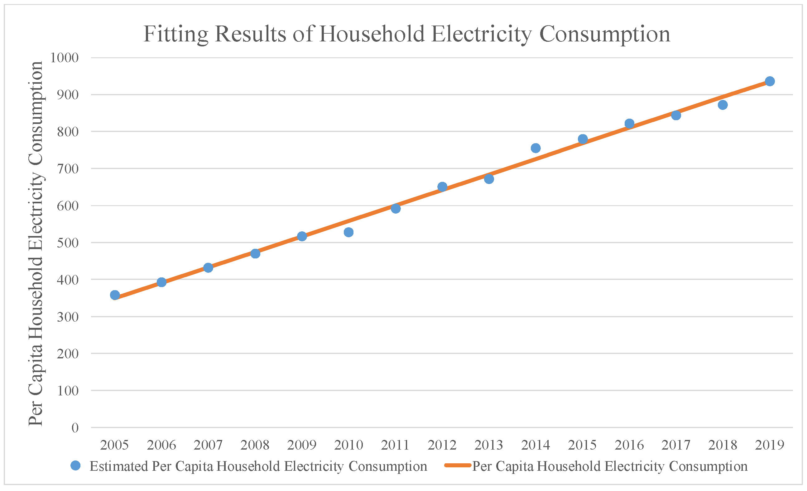
G province’s PCHEC data from 2005 to 2019 are used to fit and estimate PCHEC, and 15 years’ data as research samples are acquired.
EXCEL and R software are used for data processing in this part. A linear regression model is constructed to fit the time series of electricity consumption, and then predict G province’s household electricity consumption in 2025, 2030, and 2035. The time series function formula of household electricity consumption is assumed in Formula (A4):
Y t = a + b X t
where Y t represents PCHEC in the year t; X t , the length of time (year). Results of PCHEC are shown in Table A9:
Table A9. Historical Data of PCEC.
Year20052006200720082009201020112012
PCEC (kWh)359393432471517529593651
Year2013201420152016201720182019
PCEC (kWh)672756780822845873937
Based on the above data, the R software is used for regression analysis. Fitting output results are shown in Table A10:
Table A10. Data Fitting Results.
Coefficients Regression Statistics
Intercept307.06Multiple R0.997
X t 41.855R Square0.994
Standard Error15.089
Fitting results of household electricity consumption data are shown in Figure A1:
Figure A1. Fitting Results of Household Electricity Consumption.
Sustainability 14 08765 g0a1
The calculation formula of household electricity consumption after fitting is shown in Formula (A5):
Y t = 307.06 + 41.855 X t

Appendix B.3. Estimated Total Electricity Consumption

Based on historical data and policy adjustments, reasonable forecasts of industrial output value and population are made. Considering the above-estimated ECPUOV of the three industries, national output value structure, population, and PCHEC, estimates of G province’s total electricity consumption are shown in Table A11.
Table A11. Estimated Total Electricity Consumption of G Province.
Item2025 (Estimated)2030 (Estimated)2035 (Estimated)
G province’s GDP (CNY 100 Million) 1126,182161,043195,934
Population (10,000 Persons)12,24012,70013,000
ECPUOV of Primary Industry (kWh/CNY)0.0330.0340.035
ECPUOV of Secondary Industry (kWh/CNY)0.1030.090.078
ECPUOV of Tertiary Industry (kWh/CNY)0.0250.0220.018
PCHEC (kWh/Person/Year)118613961605
Total Electricity Consumption920010,50011,300
1 Based on 2010 Price.

References

  1. International Energy Agency. Global Energy Review: CO2 Emissions in 2021. Available online: https://www.iea.org/reports/global-energy-review-CO2-emissions-in-2021-2 (accessed on 20 May 2022).
  2. International Energy Agency. Enhancing China’s ETS for Carbon Neutrality: Focus on Power Sector. Available online: https://www.iea.org/reports/enhancing-chinas-ets-for-carbon-neutrality-focus-on-power-sector (accessed on 20 May 2022).
  3. International Energy Agency. An Energy Sector Roadmap to Carbon Neutrality in China. Available online: https://www.iea.org/reports/an-energy-sector-roadmap-to-carbon-neutrality-in-china (accessed on 20 May 2022).
  4. Zheng, B.; Wang, S.; Xu, J.X. A Review on the CO2 Emission Reduction Scheme and Countermeasures in China’s Energy and Power Industry under the Background of Carbon Peak. Sustainability 2022, 14, 879. [Google Scholar] [CrossRef]
  5. International Energy Agency. Net Zero by 2050: A Roadmap for the Global Energy Sector. Available online: https://www.iea.org/reports/net-zero-by-2050 (accessed on 20 May 2022).
  6. McKinsey & Company. Pathways to a Low-carbon Economy: Version 2 of the Global Greenhouse Gas Abatement Cost Curve. Available online: https://www.mckinsey.com/business-functions/sustainability/our-insights/pathways-to-a-low-carbon-economy (accessed on 20 May 2022).
  7. Fan, Z.G.; Hu, Q. Research on influencing factors and countermeasures of industrial carbon emission in Hebei province based on Kaya model. IOP Conf. Ser.-Earth Environ. Sci. 2020, 450, 012068. [Google Scholar] [CrossRef]
  8. Tao, Y.; Wen, Z.G.; Xu, L.; Zhang, X.; Tan, Q.L.; Li, H.F.; Evans, S. Technology options: Can Chinese power industry reach the CO2 emission peak before 2030? Resour. Conserv. Recycl. 2019, 147, 85–94. [Google Scholar] [CrossRef]
  9. Zoundi, Z. CO2 emissions, renewable energy and the Environmental Kuznets Curve, a panel cointegration approach. Renew. Sustain. Energy Rev. 2017, 72, 1067–1075. [Google Scholar] [CrossRef]
  10. Chang, K.; Chen, G.J.; Du, Z.F.; Hou, F.J.; Li, J.Q.; Chen, F. Decomposition and decoupling research of Chinese power sector carbon emissions through the consumption accounting principle. Environ. Sci. Pollut. Res. 2022, 29, 9080–9096. [Google Scholar] [CrossRef] [PubMed]
  11. Liu, J.P.; Wei, D.L. Analysis and Measurement of Carbon Emission Aggregation and Spillover Effects in China: Based on a Sectoral Perspective. Sustainability 2020, 12, 8966. [Google Scholar] [CrossRef]
  12. York, R.; Rosa, E.A.; Dietz, T. STIRPAT, IPAT and ImPACT: Analytic tools for unpacking the driving forces of environmental impacts. Ecol. Econ. 2003, 46, 351–365. [Google Scholar] [CrossRef]
  13. Wang, P.; Wu, W.S.; Zhu, B.Z.; Wei, Y.M. Examining the impact factors of energy-related CO2 emissions using the STIRPAT model in Guangdong Province, China. Appl. Energy 2013, 106, 65–71. [Google Scholar] [CrossRef]
  14. Wang, M.; Feng, C. Decomposition of energy-related CO2 emissions in China: An empirical analysis based on provincial panel data of three sectors. Appl. Energy 2017, 190, 772–787. [Google Scholar] [CrossRef]
  15. Liu, Z.; Guan, D.B.; Wei, W.; Davis, S.J.; Ciais, P.; Bai, J.; Peng, S.S.; Zhang, Q.; Hubacek, K.; Marland, G.; et al. Reduced carbon emission estimates from fossil fuel combustion and cement production in China. Nature 2017, 524, 335–338. [Google Scholar] [CrossRef] [Green Version]
  16. IPCC. 2006 IPCC Guidelines for National Greenhouse Gas Inventories. Available online: https://www.ipcc.ch/report/2006-ipcc-guidelines-for-national-greenhouse-gas-inventories (accessed on 20 May 2022).
  17. Wang, W.X.; Kuang, Y.Q.; Huang, N.S. Study on the decomposition of factors affecting energy-related carbon emissions in Guangdong province, China. Energies 2011, 4, 2249–2272. [Google Scholar] [CrossRef] [Green Version]
  18. Peter, C.; Fiore, A.; Hagemann, U.; Nendel, C.; Xiloyannis, C. Improving the accounting of field emissions in the carbon footprint of agricultural products: A comparison of default IPCC methods with readily available medium-effort modeling approaches. Int. J. Life Cycle Assess. 2016, 21, 791–805. [Google Scholar] [CrossRef] [Green Version]
  19. Wang, S.J.; Zhou, C.S.; Li, G.D.; Feng, K.S. CO2, economic growth, and energy consumption in China’s provinces: Investigating the spatiotemporal and econometric characteristics of China’s CO2 emissions. Ecol. Indic. 2016, 69, 184–195. [Google Scholar] [CrossRef]
  20. Jian, J.H.; Fan, X.J.; He, P.L.; Xiong, H.; Shen, H.Y. The Effects of Energy Consumption, Economic Growth and Financial Development on CO2 Emissions in China: A VECM Approach. Sustainability 2019, 11, 4850. [Google Scholar] [CrossRef] [Green Version]
  21. Sahoo, M.; Sahoo, J. Effects of renewable and non-renewable energy consumption on CO2 emissions in India: Empirical evidence from disaggregated data analysis. J. Public Aff. 2020, 22, e2307. [Google Scholar] [CrossRef]
  22. Sahoo, M.; Gupta, M.; Srivastava, P. Does information and communication technology and financial development lead to environmental sustainability in India? An empirical insight. Telemat. Inform. 2021, 60, 101598. [Google Scholar] [CrossRef]
  23. Mohini, G.; Seema, S.; Malayaranjan, S. Determinants of ecological footprint and PM2.5: Role of urbanization, natural resources and technological innovation. Environ. Chall. 2022, 7, 100467. [Google Scholar] [CrossRef]
  24. Ali, H.S.; Sahoo, M.; Alam, M.M.; Tijjani, I.I.; Al-Amin, A.; Ahmed, A. Structural transformations and conventional energy-based power utilization on carbon emissions: Empirical evidence from Pakistan. Environ. Dev. Sustain. 2022. [Google Scholar] [CrossRef]
  25. Villanthenkodath, M.A.; Gupta, M.; Saini, S.; Sahoo, M. Impact of Economic Structure on the Environmental Kuznets Curve (EKC)hypothesis in India. Econ. Struct. 2021, 10, 28. [Google Scholar] [CrossRef]
  26. Zhou, L.Y. Study on the influence of urban construction land expansion on carbon emission based on VAR Model—A case study of Nanchang City. IOP Conf. Ser. Earth Environ. Sci. 2021, 769, 022071. [Google Scholar] [CrossRef]
  27. Ma, Y.Y.; Zhang, Z.X.; Zhang, F.F.; Liu, Z.Y. How might Shandong achieve the 2030 CO2 emissions target? A system dynamics analysis from the perspective of energy supply-side structural reform in China. Int. J. Glob. Warm. 2019, 17, 357–372. [Google Scholar] [CrossRef]
  28. Leitao, J.; Ferreira, J.; Santibanez-Gonzalez, E. New insights into decoupling economic growth, technological progress and carbon dioxide emissions: Evidence from 40 countries. Technol. Forecast. Soc. Chang. 2022, 174, 121250. [Google Scholar] [CrossRef]
  29. Huang, Y.S.; Xu, J. Research on Carbon Emission Measurement of Electricity Sector Based on Scenario Analysis Method. Appl. Mech. Mater. 2013, 367, 327–332. [Google Scholar] [CrossRef]
  30. Song, C.; Zhao, T.; Wang, J. Analyzing driving forces of China’s carbon emissions from 1997 to 2040 and the potential emission reduction path: Through decomposition and scenario analysis. Clean Technol. Environ. Policy 2021, 24, 1219–1240. [Google Scholar] [CrossRef] [PubMed]
  31. Zhang, C.; Su, B.; Zhou, K.L.; Yang, S.L. Decomposition analysis of China’s CO2 emissions (2000–2016) and scenario analysis of its carbon intensity targets in 2020 and 2030. Sci. Total Environ. 2019, 668, 432–442. [Google Scholar] [CrossRef]
  32. Li, L.C.; Meinrenken, C.J.; Modi, V.; Culligan, P.J. Short-term apartment-level load forecasting using a modified neural network with selected auto-regressive features. Appl. Energy 2021, 287, 116509. [Google Scholar] [CrossRef]
  33. Seker, M. Long term electricity load forecasting based on regional load model using optimization techniques: A case study. Appl. Energy 2021, 44, 21–43. [Google Scholar] [CrossRef]
  34. Wang, H.; Zhou, P.; Xie, B.C.; Zhang, N. Assessing drivers of CO2 emissions in China’s electricity sector: A metafrontier production-theoretical decomposition analysis. Eur. J. Oper. Res. 2018, 275, 1096–1107. [Google Scholar] [CrossRef]
  35. Jiang, H.J.; Geng, Y.; Tian, X.; Zhang, X.; Chen, W.; Gao, Z.Y. Uncovering CO2 emission drivers under regional industrial transfer in China’s Yangtze River Economic Belt: A multi-layer LMDI decomposition analysis. Front. Energy 2020, 15, 292–307. [Google Scholar] [CrossRef]
  36. Harrathi, N.; Almohaimeed, A. Determinants of Carbon Dioxide Emissions: New Empirical Evidence from MENA Countries. Int. J. Energy Econ. Policy 2022, 12, 469–482. [Google Scholar] [CrossRef]
  37. Sadr, N.R.; Bahrdo, T.; Taghizadeh, R. Impacts of Paris agreement, fossil fuel consumption, and net energy imports on CO2 emissions: A panel data approach for three West European countries. Clean Technol. Environ. Policy 2022, 24, 1521–1534. [Google Scholar] [CrossRef]
  38. Shi, H.T.; Chai, J.; Lu, Q.Y.; Zheng, J.L.; Wang, S.Y. The impact of China’s low-carbon transition on economy, society and energy in 2030 based on CO2 emissions drivers. Energy 2021, 239, 122336. [Google Scholar] [CrossRef]
  39. Li, A.J.; Zhang, A.Z.; Zhou, Y.X.; Yao, X. Decomposition analysis of factors affecting carbon dioxide emissions across provinces in China. J. Clean. Prod. 2017, 141, 1428–1444. [Google Scholar] [CrossRef]
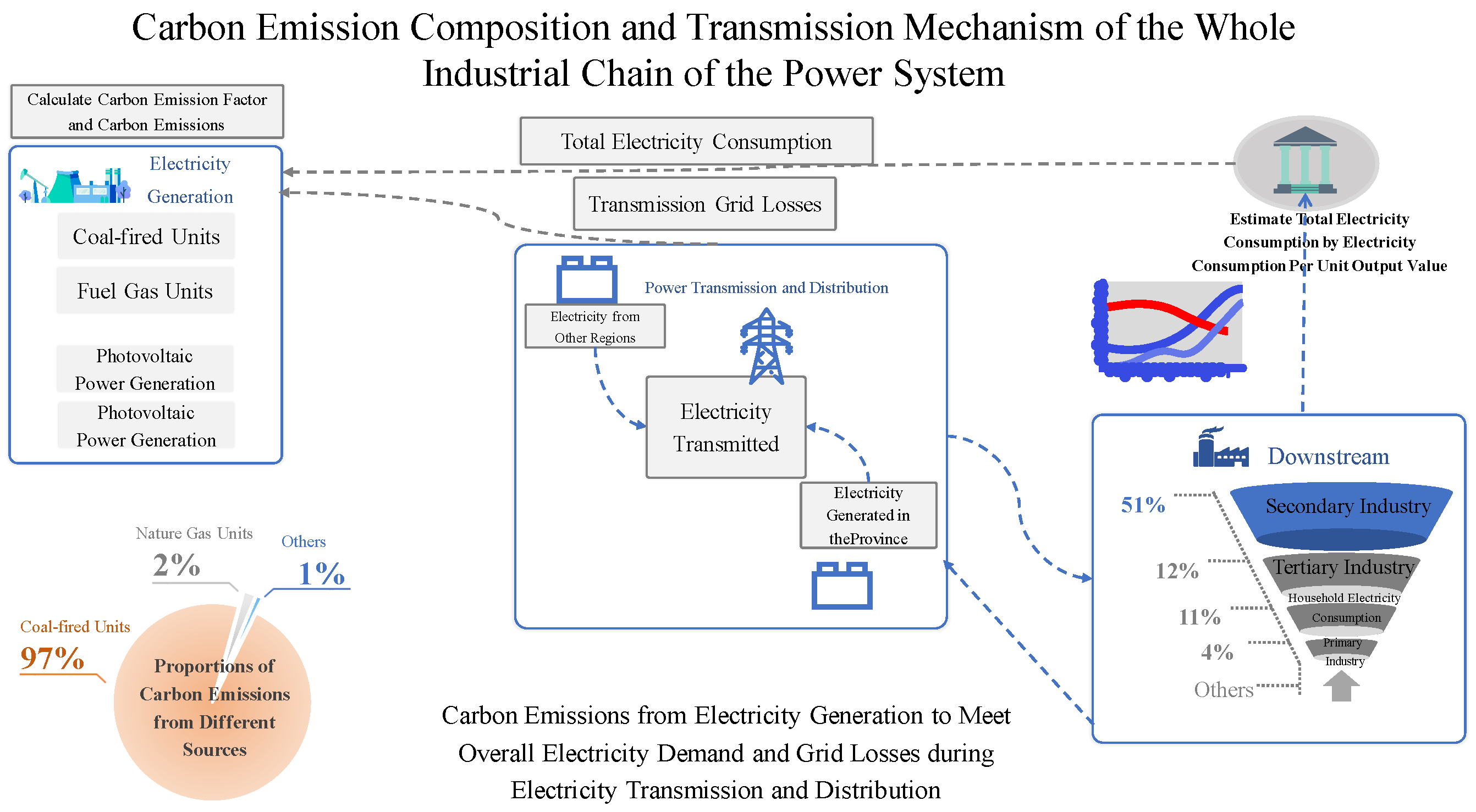
Figure 1. Carbon Emission Composition and Transmission Mechanism of the Power Whole Industrial Chain.
Sustainability 14 08765 g001
Figure 2. REF Carbon Emission Curve.
Sustainability 14 08765 g002
Figure 3. LC Carbon Emission Curve.
Sustainability 14 08765 g003
Figure 4. SC Carbon Emission Curve.
Sustainability 14 08765 g004
Table 1. Historical Data of Carbon Emission Factor.
Year A t Q t η t α t α t -Model ( R 2 ) 1
201068.50%80.58%40.32%0.56720.57140.967
201177.22%82.41%40.86%0.57930.5903
201270.73%78.16%41.13%0.55520.5515
201365.07%78.42%41.27%0.55380.5418
201461.05%77.08%41.69%0.5140.5222
201555.68%75.32%41.00%0.50580.5113
201652.73%70.61%41.69%0.45690.4708
201758.21%72.79%42.41%0.46460.484
201857.66%71.79%43.61%0.45520.4629
201953.77%66.58%43.00%0.4110.4337
202051.25%67.87%42.70%0.43380.4403
1 Goodness of Fit.
Table 2. Estimated Carbon Emission Factors.
Item2021202220232024202520302035
REF0.44970.43020.42040.42270.41380.39580.3993
LC0.44970.43070.41680.40810.3940.3090.2727
SC0.44970.45150.43820.43250.42070.34460.315
Table 3. Estimated Total Electricity Consumption in G Province Based on ECPUOV.
Item 20192020202520302035
Total Population (10,000 Persons) 11,52111,64012,24012,70013,000
PCHEC (kWh/Person) 937972120014001600
Primary Industry36643772441648475310
Economy (CNY 100 Million)Secondary Industry36,66837,71648,95859,68369,106
Tertiary Industry50,33252,80373,05996,46512,1518
Primary Industry0.0320.0330.0330.0340.035
CPUOV (kWh/CNY)Secondary Industry0.1120.1120.1030.0900.078
Tertiary Industry0.0270.0270.0250.0220.018
Primary Industry117124146165186
Electricity Consumption (100 Million kWh)Secondary Industry41204209504353715390
Tertiary Industry13801435182621222187
Residents10791132146917782080
Total Electricity Consumption (100 Million kWh) 66966926920010,50011,300
Table 4. G province’s Grid Loss Rate.
Item2021202220232024202520302035
REF3.98%3.98%3.98%3.98%3.98%3.98%3.98%
LC3.96%3.95%3.94%3.90%3.80%3.80%3.80%
SC3.96%3.95%3.94%3.90%3.80%3.75%3.75%
Table 5. REF Carbon Emissions.
Variable20202021202220232024202520302035
T c t (100 Million Tons)2.162.922.772.832.973.013.103.36
S c t (100 Million Tons)2.042.772.632.692.822.862.943.18
P c t (100 Million Tons)0.120.150.140.140.150.150.160.18
Table 6. LC Carbon Emissions.
Variable20202021202220232024202520302035
T c t (100 Million Tons)2.162.922.772.812.862.862.422.29
S c t (100 Million Tons)2.042.772.632.672.722.722.302.17
P c t (100 Million Tons)0.120.150.140.140.140.140.120.12
Table 7. SC Carbon Emissions.
Variable20202021202220232024202520302035
T c t (100 Million Tons)2.162.923.093.163.283.312.942.90
S c t (100 Million Tons)2.042.772.943.013.123.162.802.76
P c t (100 Million Tons)0.120.150.150.150.160.150.140.14
Publisher’s Note: MDPI stays neutral with regard to jurisdictional claims in published maps and institutional affiliations.