Abstract
Eco-driving is a keystone in energy reduction in railways and a fundamental tool to contribute to the Sustainable Development Goals in the transport sector. However, its results in real applications are subject to uncertainties such as climatological factors that are not considered in the train driving optimisation. This paper aims to develop an eco-driving model to design efficient driving commands considering the uncertainty of climatological conditions. This uncertainty in temperature, pressure, and wind is modelled by means of fuzzy numbers, and the optimisation problem is solved using a Genetic Algorithm with fuzzy parameters making use of an accurate railway simulator. It has been applied to a realistic Spanish high-speed railway scenario, proving the importance of considering the uncertainty of climatological parameters to adapt driving commands to them. The results obtained show that the energy savings expected without considering climatological factors account for 29.76%, but if they are considered, savings can rise up to 34.7% in summer conditions. With the proposed model, a variation in energy of 5.32% is obtained when summer and winter scenarios are compared while punctuality constraints are fulfiled. In conclusion, the model allows the operator to estimate better energy by obtaining optimised driving adapted to the climate.
1. Introduction
The current global context of sustainable development urges all countries to mitigate the consequences of climate change. It is also a time when the current trend of societies in developed countries is to concentrate the population in huge metropolia. The railway sector plays a vital role in transporting people between these large metropolitan areas. Its immediate future lies in making the train more attractive to potential users. In this regard, high-speed railways (HSR) has been an advance, providing a fast and comfortable transport mode for long-distance services. HSR is considered an efficient transport mode and is part of the strategy to avoid the pollution produced by the massive use of private vehicles. Europe is leading among the developed countries in managing decarbonisation in all sectors with imminent effect. In this way, the Sustainable Development Goals (SDGs) are the main framework in which measures have to be taken. Therefore, the most immediate action to carry through by society, administrations, and companies is to develop technology by making it more efficient in terms of emissions of greenhouse gases.
This rational use of energy is particularly relevant for the transport sector because of the massive amount of energy required in developed countries [1,2], especially when the trend is towards unification into an electrified system. In this manner, railway transport is the most efficient in energy consumption and pollution emission. Railway operations account for a low percentage of energy consumption, but, even so, it is a large consumer and, therefore, its efficiency is susceptible to being improved [3]. Railway operators, national infrastructure managers, and other companies in the sector apply all kinds of technological developments in order to minimise the energy consumption associated with train operations, always considering the comfort and safety requirements.
Eco-driving is one of the most popular methods for optimising energy consumption in railway operations because it can be applied in the short term, providing important energy reduction results [4]. Eco-driving is the obtention of the speed profile with the minimum energy consumption associated. The eco-driving speed profile is calculated for a specific target running time considering the previously designed timetable [3,5,6,7,8,9,10,11].
Different eco-driving strategies have been analysed in the academic literature. In some simple scenarios, driving through speed regulation has been simulated [1,12,13,14]. Other studies have proposed design by coast-remotoring cycles, having upper and lower speed limits [15,16,17] or considering coasting points along the railway line [18,19,20,21,22]. Previous strategies are appropriate for short routes on metro lines but are not very efficient for longer railway lines as the HSR lines. The speed regulation without braking has been demonstrated as an efficient and easily executed eco-driving strategy for high-speed railway lines [23,24].
The production of speed profiles with the minimum energy consumption requires an optimisation model that can return the best combination of eco-driving strategies. In study [18], the initial study on eco-driving was developed. This work applies Pontryagin’s Maximum Principle to a simplified train dynamics model, obtaining optimal driving modes as maximum acceleration, cruising, coasting, and maximum braking. The studies developed subsequently to [18] have improved the dynamic model of simulation, and the different optimisation techniques implemented are classified in study [25] as analytical and numerical methods.
Most of the analytical methods are developed based on the optimal control theory. Pontryagin’s Maximum Principle is used in these methods to find the best energy efficiency solutions and apply algorithms to obtain the optimal switching points between the efficient regimes. These algorithms are based on Dynamic Programming [26,27,28,29], constructive algorithms [1,21,30,31], Sequential Quadratic Programming [32], and the method of Lagrange Multipliers over the discretised problem [33]. Other methods transform the situation into a non-linear problem [34]. The analytical methods are used to provide the optimal solution but, considering the complexity of the problem to be solved, a series of simplifications have to be made in the train model. Due to the simplifications, inaccuracies can be obtained in the results generated, and may require recalculations in real applications [13].
On the other hand, numerical methods have been used for solving the problem of efficient driving in railway operations as well. These methods are flexible enough to be used without reducing the complexity of the train model by using detailed simulation models, adjusting the comfort and driving requirements. Thus, these methods can be used to fulfil any need or constraint in real situations.
Among these numerical methods are Artificial Neural Networks, being used for the optimisation of the coasting points [35], the optimisation of the coasting speed for a Mass Rapid Transit System considering energy cost and travelling time cost [36], and for calculating a new indicator to characterise a railway traffic driving smoothness [37]. Nature-inspired optimisation algorithms such as Genetic Algorithm (GA) have been widely applied for determining the speed profile which minimise the energy consumption [2], the optimal coasting points [19], and the optimum train speed along the journey [27]. A single optimise train trajectory considering net energy between adjacent DC substations is described in [38]. In study [39], it is jointly optimised by means of a GA for the timetable and the speed profile. A coasting point control method is developed in [40,41,42] based on GA to determine its number and position. Multi-population Genetic Algorithm (GA) is used in [43] to reduce energy consumption in a subway system with multiple stations, and in [44] in order to determine the acceleration, cruising and coasting points. GA combined with fuzzy logic is used in [16] to optimise energy traction by trading-off reductions in energy against time, in study [23] to find the economical pattern for an HSR balancing energy and running time, and used in studies [45,46] to calculate optimal speed profiles considering uncertainty in manual driving. Direct search algorithms have been applied to minimise energy traction in [47] while Brute Force algorithm is used in [48] to minimise energy consumption in substations. A Monte Carlo Simulation model was proposed to determine the system energy flow considering regenerative braking trains [49]. Differential Evolution has been presented in [50] to optimise railway operation. Optimisation by minimising energy traction is carried out by Simulated Annealing in [51] and searching optimal coasting points in [52]. On the other hand, multi-objective models have been developed using numerical methods. Among them, Indicator Based Evolutionary Algorithm (IBEA) was proposed to optimise both the running time and energy consumption [53]. Non-dominated Sorting Genetic Algorithm II (NSGA-II) is used in [54] to design ATO CBTC speed profiles to minimise energy traction and in [55], its performance is compared with Multi-Objective Particle Swarm Optimisation (MOPSO) generating the Pareto curve for real cases of the Madrid Underground. Ant Colony Optimisation can be seen in [27], proposing a distance-based train trajectory optimising the train trajectory, and in [56] to achieve the optimal driving strategy. Finally, a MOPSO algorithm is used in [57] to design efficient speed profiles for the ATO of the trains of a metro line.
With the purpose to obtain accurate results, it is important not only to use detailed simulation models but also to take into account the possible uncertainties that emerge from the HSR operation. These uncertainties can be classified in three groups: limitations in the movement authority produced by signals or preceding trains [58,59], variability in the manual operation of the train [45], and the climate conditions. While the first two uncertainty sources have been widely studied, climate conditions have not been deeply considered in the eco-driving problem.
Most academic works focus on winter scenarios in Northern Europe to forecast delays or disruptions in traffic operation. Some studies have reviewed the issues during winter railway operations caused by snow and ice in Nordic countries [60]. In study [61], impact of humidity, temperature, ice, and snow depth on the occurrence of delays in high-speed operation in Sweden has been analysed through a Cox model and Markov chain model. A train delay prediction model with weather data has been designed in [62] and tested on two high-speed railway lines in China. The Nordland railway line has been assessed in [63], where extreme cold weather is a crucial factor related to delays and low punctuality. Other papers have focused on service delay time and its exposure time to bad weather [64]. A combination of fuzzy theory and rough sets under adverse weather conditions has been used to contribute to the forewarning method for train operation in [65]. Causal relationships between extreme weather patterns and derailments on railway turnouts have been investigated by means of Fuzzy Bayesian Network model [66]. The impact on freight railways in winter weather in Northern Europe has been discussed [67]. In study [68], an estimation of the effects of weather conditions on railway operator performance of passenger train services has been carried out, focusing on infrastructure disruptions. In study [69], a model to capture the cascade dynamics of delay propagation on railway networks under inclement weather has been presented.
As a general rule, climatological factors are considered random variables and instantly excluded from the models considered by railway operators. However, in HSR, the running resistance is the major factor determining the trains’ energy consumption. Climatic conditions such as wind or air density can produce significant variations in running resistance value. Therefore, climatology plays an important role in the energy that high-speed trains demands. Previous reasons motivate this paper to generate a new model to quantify the climatological affection in railway operation, both in energy consumption and in running time. Climatology has a great variability due to the impossibility of having complete knowledge of all the variables that model its behaviour. Therefore, climatic conditions such as pressure, temperature, and wind have been modelled by means of fuzzy logic [70]. This way, this affection is included in the running resistance, given the vagueness in the knowledge of these variables.
The main advantage of fuzzy logic modelling is the ability to handle imprecise or incomplete information. Additionally, a positive feature is its flexibility and simplicity to be developed and implemented to obtain efficient calculations. That is why many studies have applied fuzzy logic in train operation models. In study [71], the train service provider and the infrastructure provider have been modelled as software agents, and the negotiation for a train schedule and the associated track access charge as a prioritised fuzzy constrain satisfaction problem. In study [72], predictive fuzzy control is used for carrying out the train dwell-time control in an event-driven framework. A methodology for predictive fuzzy control in an event-driven environment for multi-objective decision making on DC railway systems has been presented in [73]. In study [74], an approach within the fuzzy framework for tackling the complexity of multidimensional service evaluations and the judgment on the goodness of the schedule has been proposed. In study [75], the authors investigated a passenger train timetable problem with fuzzy passenger demand. The paper presented by [76] exposed a framework to evaluate the logistics performance of intermodal freight transportation by applying fuzzy set techniques. A multilevelled distributed railway traffic fuzzy control system is proposed in [77]. An assistant support system for railway traffic control is described in [78] making use of fuzzy knowledge. A fuzzy optimisation model for rescheduling high-speed timetables is proposed in [11], focusing this work on punctuality and passengers’ affection without considering energy minimisation. In studies [79,80], a fuzzy model is proposed for an Automatic Train Control system. In studies [45,59], uncertainty in the manual driving application of the speed regulation command is modelled using fuzzy numbers. In study [16], the optimal speed profile in urban DC railways is found with a GA, where the energy consumption and the running time are the fuzzy results. A fuzzy model of delays and punctuality constraints is proposed in [46] for the offline design of timetables when efficient driving is applied. The algorithm proposed in [54] is used for urban ATO operation including uncertainty in the mass, generating optimal energy–time Pareto curves of speed profiles. Fuzzy logic is applied in [81] to detect the railway wheelset conicity as a measure of the deterioration. In study [82], a fuzzy model is used to evaluate the potential risks of railway crossings. As can be seen, climatological parameters and their associated uncertainty have not been modelled previously; therefore, this possible affection to the railway operation has not been considered.
The main contribution of this paper is the introduction of climatological parameters in the eco-driving optimisation model. The proposed model allows an efficient driving design considering the uncertainty due to climate conditions by means of fuzzy modelling. Climatological parameters are not typically considered in the design of speed profiles, and they could affect the running time and energy consumption.
The optimisation model is based on a Genetic Algorithm combined with fuzzy parameters. This algorithm applies a search process that optimises a driving holding speed without a braking commands set that can be easily applied by human drivers. Applying these commands generates the efficient driving with punctuality requirements at the destination. Using a detailed simulation platform makes solving all possible scenarios possible when the climatological parameters vary according to the proposed model. This methodology can also be applied to quantify the error obtained in the expected energy saving if climate conditions are not initially considered in the optimisation of the railway operation. The model has been applied in a simulation test based on real data of a Spanish HSR, to compare scenarios where different wind and air pressure conditions are considered.
The paper is organised as follows: Section 2 describes the simulation model in which the weather parameters are included. The uncertainty associated with the climatological parameters is modelled in Section 3. Section 4 is a description of the optimisation model developed to generate efficient driving. Section 5 analyses the case study and presents the results obtained for a real high-speed railway line using the models proposed in previous sections. A discussion of the proposed procedure and the results are presented in Section 6. At the end of the document, the bibliographical references and previous academic studies from which information for the present analysis has been obtained are presented.
2. Simulation
2.1. Simulation Model
The simulation model is described in this section. This model is detailed in [45], and the results provided by the simulation were compared with real data of a Spanish HSR to validate the simulator. Differences of 1.2% for the running time and differences of 0.4% when compared with the energy consumption were shown. The model was used from [45] to design eco-driving in a high-speed line, and measurements were recorded. As a result, energy savings between 20% and 34% were measured in commercial services. It was a detailed discrete event deterministic simulation model, that combines next-event and fixed-discrete time steps for advancing the simulation clock [83,84]. The simulation model takes several input data related to the rolling stock involved in the operation and related to the railway line:
- ❖
- Rolling stock.
- i.
- Physical parameters: mass of the train, the mass of the load, length, maximum speed, rotatory inertia, and adhesion traction.
- ii.
- Traction effort curve, braking effort curve, running resistance coefficients, energetic and power systems and auxiliary systems consumptions.
- ❖
- Railway line. Includes Kilometric Points of relevant information as stations (K.P.), grades, track curvatures, speed limits, tunnels, and grade transitions considering the length of the train and the electric neutral zones.
The equation that models the motion of the train at each simulation step considering the forces acting on the train is:
where
- a is the acceleration of the train.
- Fm is the motor force.
- R is the running resistance of the train defined by the Davis formula (Equation (7)).
- Fg is the force due to the railway grades.
- Fr is the force due to track curvature.
- meq is the equivalent mass.
By definition, the acceleration of the train in every step of the simulation is:
The equivalent mass, effective mass or inertial mass can be calculated by:
where
- m0 is the empty train mass.
- ml is the load mass.
- λ is the dimensionless rotating mass factor.
Force due to gradient (Equation (4)) shows acceleration due to gravity effect, considering uphill or downhill motion. Therefore, the force due to gradient profile can be written as:
where
- g is the gravity acceleration.
- θ is the slope angle.
Given the small values of slope angle in typical railway tracks, Equation (4) can be written as:
where
• p is the gradient of the track (mm/m or ‰).
Likewise, the force due to the track curvature can be expressed as follows:
where
- Kr is an empirical constant defined by track gauge.
- r is the radius of track curvature.
The traction effort or motor force (Fm) is bounded by a maximum value of the electrical traction effort curve and a maximum electrical braking effort curve both dependent on the train speed. The simulation model considers at every moment the speed limits established along the rail track by the railway administration. Speed limits are defined by stretches along the railway where the train must drive respecting the maximum speed limit considering the total length of the train. When a train passes through a neutral zone, auxiliary systems cannot be fed from a catenary, and motors apply at least a constant braking effort to maintain the charge of the batteries that feed auxiliary systems along neutral zones.
Running resistance is the model that defines and groups a series of resistances opposing the train’s movement. These include mechanical resistances (rolling and internal friction), air intake resistances (for engine cooling and passenger air renewal), and aerodynamic resistance [85]. The running resistance is modelled with a second-degree equation dependent on the instantaneous velocity and defined by the Davis expression [86]:
where
- a is a constant related to the mechanical resistance to the motion.
- b is a constant related to the resistance due to the air inlet in the train.
- c is a constant related to the aerodynamic resistance.
- k is the tunnel factor.
- vtrain is the velocity of the train.
The Davis formulae and similar expressions of a polynomial nature are models of reality. Each term of this equation refers to different physical components of the total running resistance. However, it must be considered that these polynomials are fitted models of highly complex phenomena that interact themselves. Therefore, although for general purposes certain approximations can be estimated, in reality, they are not completely accurate and do not represent reality in its entirety. Likewise, within the running resistance model, there are parameterised coefficients (a, b and c) that represent different oppositions to the movement of the train. These values are experimental, complex to define, and depend on the physical characteristics of the rolling stock. In order to obtain them, manufacturers test their trains and their relationships with the resistances generated. These coefficients are the nominal values, so they have been evaluated under standard conditions of pressure and temperature given by the International Standard Atmosphere, ISA (ISO, 1975: T = 15 °C; ρ = 1.225 kg/m3).
The term of the running resistance model (Equation (7)) that is not related to the effect of the air outside the train is called mechanical resistance. In this term, the coefficient a is involved. In the most general case, it is derived from the frictional resistance between mechanical components, rail-to-wheel contact, track irregularities, and energy losses in the traction and suspension equipment of the vehicles due to the oscillating or parasitic movements of the suspended mass.
The term of the train speed-dependent running resistance corresponds, mainly, to the resistance caused by the air intake of the train. In trains, there is a constant and noticeable air flow, necessary for cooling engines and other equipment as well as that required for air renewal for passengers. This term is related to the b coefficient of the running resistance model.
The so-called aerodynamic running resistance is the longitudinal force that opposes the train’s movement as a consequence of the interaction between the train and the surrounding air with which it collides and envelops it. The coefficient c is responsible for modelling this resistance.
The tunnel factor k increases the quadratic term of the running resistance model when the train runs through a tunnel due to the increased air friction against the outer surface of the train. When a tunnel is not involved in the simulation, the factor takes the value 1.
Equations (1)–(7) describe the motion of the train in next-event and fixed-discrete simulation steps, limited by speed limits, calculating braking curves to stop at the arrival point or station point with comfort and safety requirements.
The model related to the energy consumed by the train measured at the pantograph Epantograph is expressed as shown in Equation (8) while the train energy consumption estimated at the electrical substation (Esubstation) is defined by means of Equation (9):
where
- Ppantograph is the electrical power consumed by the train measured at the pantograph.
- Psubstation is the estimation of the power consumed at the substation.
Previous calculus requires some other equations to complete the model:
where
- Pmec is the mechanical power.
- Paux is the power consumed by the auxiliary systems.
- ηT is the electrical chain efficiency for the traction case.
- ηB is the electrical chain efficiency for the braking case.
- V is the nominal line voltage.
- cos φ is the power factor.
- r(s) is the electrical line resistance.
- nzstart and nzend are the initial and final position of every neutral electrical zone.
2.2. Climatological Model
The following section focuses on the running resistance variation when the railway operation is developed under real climatological circumstances. Initially, the influence of the variation of density along the railway line due to altitude changes has been modelled. Then, the wind’s influence on the running resistance model is incorporated. When motion equations are applied (Equations (1)–(7)) for simulating the train’s driving in a railway line, it is supposed that pressure and temperature values are constant along the whole line under standard conditions, given by the International Standard Atmosphere [87]. Thus, Equation (7) is just modified by the velocity of the train and it incorporates coefficients, b and c given by the manufacturer. For that reason, previous coefficients are also constant along the railway operation in absence of wind and they are always the same for each line, no matter the geographical location and the season of the year considered for the railway operation. The purpose of this section is to include in the simulation model the influences on the running resistance with climatological considerations of pressure, temperature, and wind.
The railway operation can occur between points of different altitudes, and it is, therefore, to be expected that the model must deal with this variation along the railway line. In summary, throughout the journey, the air density will vary due to the change in altitude and this variation will modify the running resistance equation according to the model described below. When the train runs on a line without wind, the running resistance term can be defined by Equation (7). In the running resistance model, lineal and quadratic terms vary as a function of train speed. In the quadratic term, the coefficient can be defined by the general aerodynamics equation as shown below, according to the quasi-steady theory [88]:
where
- c is the aerodynamic coefficient of the running resistance model (Equation (7)).
- ρISA is the density of the air under standard conditions [87].
- A is the cross-sectional area.
- Fd is the drag force.
From Equation (15), it is deduced that factor c of the Davis formula is dependent on the density of the air and, therefore, on its variation. Finally, with the previous information, the coefficient c is parameterised as follows, varying with density and considering standard weather conditions as a reference [89]:
Finally, when all information related is considered, the running resistance model can be written as follows. However, this equation models the situation where the train is running without being influenced by the wind:
In this manner, a main and essential task is to know the air density at every point or analyse the stretch along the railway line. The density is a function of the temperature and pressure of the air, and its relationship can be expressed by the equation of state defined in the ideal gas law as follows:
where
- ρ is the density.
- p is the pressure.
- R is the ideal gas constant.
- T is the temperature.
Pressure and temperature values strongly depend on the meteorological conditions given a specific area due to its geographical characteristics and the year’s season. Therefore, considering the climatological model, they can be significantly different from one area to another. This work analyses these differences, which are present in the variations along the railway line.
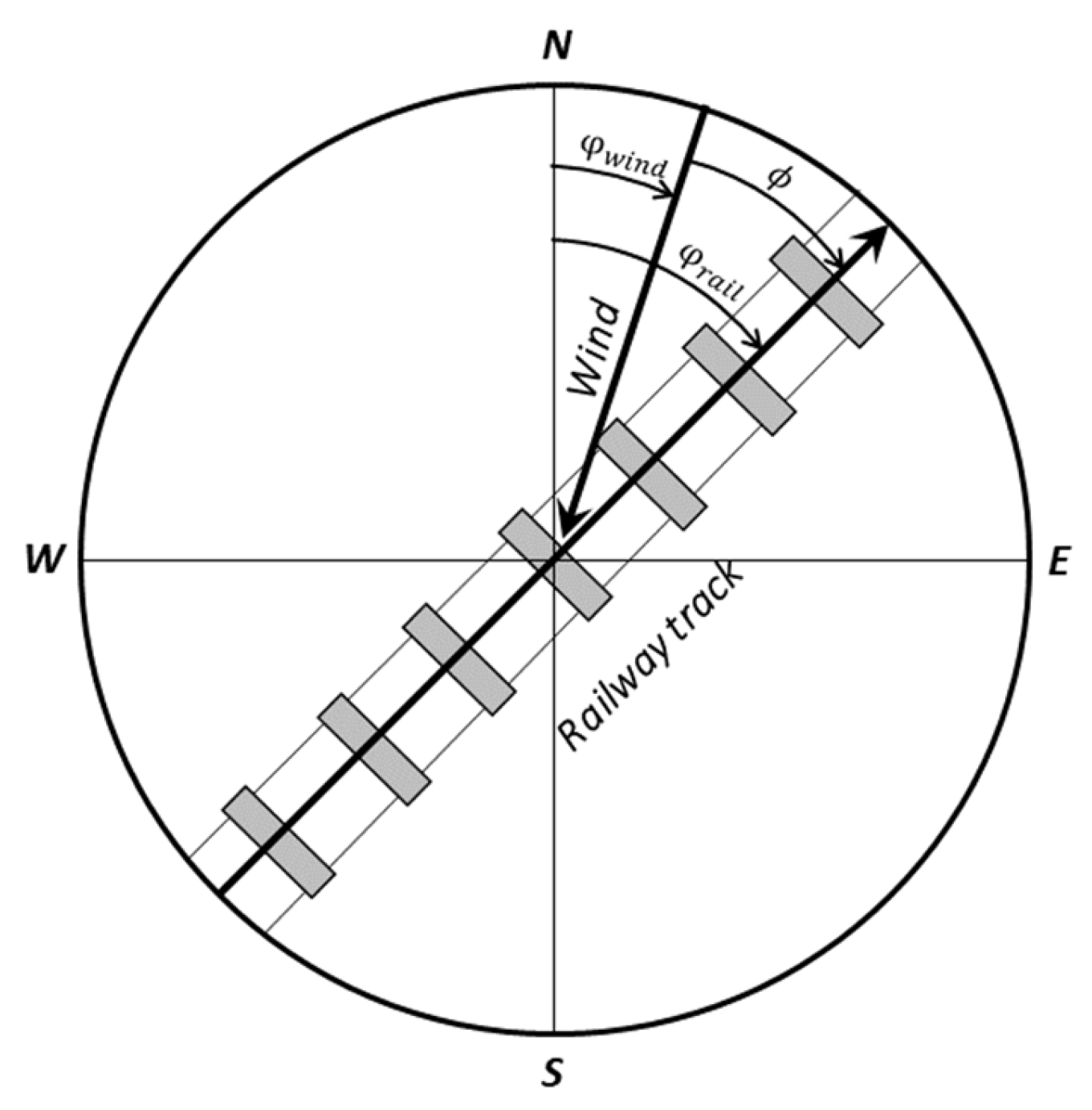
On the other side, the running resistance force is also significantly affected by the wind and its variation along the route. The influence of the wind is modelled by the combination of its intensity, or wind speed, and the angle of incidence in each stretch relative to the train () [88,89,90]. The train speed relative to the wind is the train speed minus the wind speed vectors, as it can be seen in Figure 1. Figure 2 shows the reference frame considered in this work where angle (Equation (19)) is the principal parameter to model the wind influence in the railway operation.
where
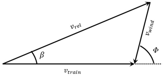
Figure 1.
Velocities diagram.

Figure 2.
Reference frame.
Running resistance model, given by Equation (7), is valid just when the wind has not been considered, so the model has to be modified, now influenced by the speed of the train and wind vectors, as shown in Figure 1. The modification consists of replacing the train speed in Equation (7) by the train speed relative to the wind, which is equivalent to considering zero wind in the original equation:
Besides and in addition to the previous model, it has to be considered that factor c also depends on the angle β as shown in Figure 1. Yaw angle can be calculated using Equation (21).
To get the final model for the running resistance of a train, the relative train speed must be calculated, determining the simulation model as follows:
Equation (23) is proposed in [91]. This expression establishes the variation of the constant according to the angle β. This is an empirical expression and becomes meaningless when β > 30°. An angle with such magnitude for typical speed values in operation would imply extreme winds, which would affect the train operation or could lead to the total suspension of the service.
where
• c(ρ) is the value of c when density variation is considered according to Equation (16).
Finally, the variable running resistance considering climatological factors is modelled as:
When the train runs through a tunnel, the force exerted by the influence of the wind shall not be considered. Therefore, for the sections simulated in a tunnel, the expression for the running resistance must be modelled with an expression that considers the train speed as input data, including the tunnel factor in the quadratic term. As applicable, it is used a k parameter as the tunnel factor:
Pressure, temperature and wind models have been discretised along the railway line. If the altitude suffers any variation along the journey, the model can deal with the change by measuring the impact of the air density variance. Two different reasons have justified the division or discretisation along the railway line. Firstly, the variability of the wind makes necessary a partition along the line where the climatological and geographical characteristics determine the main direction in which the wind blows. And secondly, the change of directions taken by the train along the railway line has been dealt implementing stretches where it can be supposed that the relative angle between the wind and the train movement is approximately constant along a straight line. Hence, the proposed wind model considers both the railway track angle and the incidence wind angle to be parametrised. In conclusion, previous considerations allow the simulation model of the train movement to deal with the wind behaviour’s complexity without compromising the final results’ accuracy.
3. Fuzzy Climatological Model
This paper quantifies the relevance of the climatological factors and their variation by modelling them with their associated uncertainty during railway operation by means of a climate fuzzy model.
The parameters modelled by fuzzy numbers [92] are defined in Section 2.2: the pressure and temperature defining, consequently, the density, and the intensity and the angle of incidence of the wind.
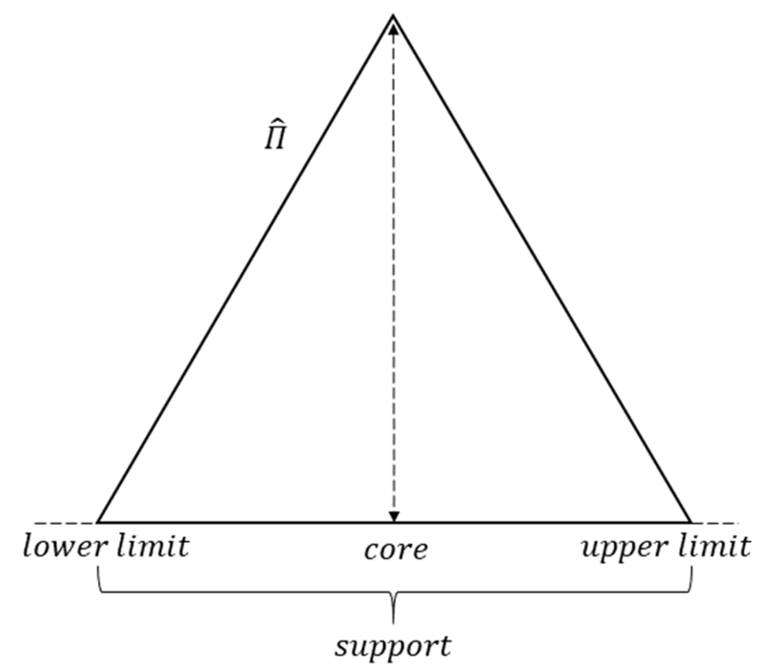
Among the many possibilities for the membership function of the fuzzy numbers: piece-wise linear [93], linear, hyperbolic, exponential and S-shaped [94,95], climatological factors have been defined as triangular fuzzy numbers. But the model proposed in this paper would be applicable if any other shape is utilised to model climatological parameters’ uncertainty. Each of the fuzzy numbers, the temperature, barometric pressure, air density, wind intensity (or speed) and the angle of incidence of wind are defined by the shape shown in Figure 3. Therefore, a fuzzy number is defined by its core, its lower limit and its upper limit of the support.

Figure 3.
Triangular fuzzy number.
Fuzzy pressure (), fuzzy temperature (), fuzzy wind speed () and fuzzy angle of incidence () have been defined for every division realised along the railway line in order to get a more detailed climatological model on railway track sections as explained in Section 2.2.
The running time is calculated from the indicated fuzzy parameters and the model input data (train and railway line, Section 2.1). This result will be a fuzzy parameter due to the uncertainty associated with some of the calculation parameters. In the proposed fuzzy model, the punctuality constraint is imposed on the fuzzy running time, which must be less or equal to the objective running time:
The punctuality constraint can be expressed either as a measure of the possibility of arriving at the scheduled time or as a measure of the necessity of fulfiling that objective. Thus, if it is expressed as a measure of the possibility αρ, the expression is:
The corresponding necessity measure, in this case, is 0:
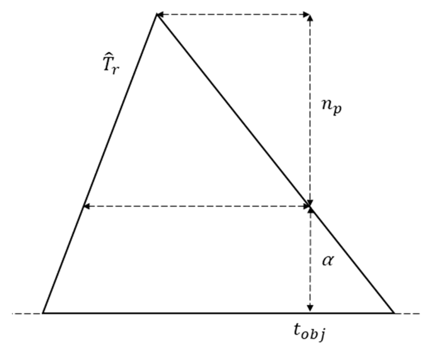
If the punctuality constraint is expressed as a measure of the required necessity , (Figure 4) the expression is:
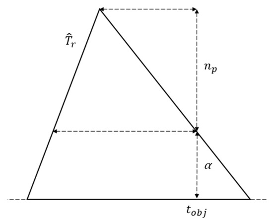
Figure 4.
Fuzzy running time.
The corresponding possibility measure, in this case, is 1:
4. Eco-Driving Optimisation with Fuzzy Parameters
Having introduced the climatological fuzzy model and how it affects the train motion simulation model, the objective is now to present the driving optimisation model. This optimal driving will be constructed as a combination of efficient commands considering coasting points known as Command Matrix (Cm). Then, the problem and proposed algorithm for the problem resolution will be presented: Genetic Algorithm with Fuzzy Parameters (GA-F).
4.1. Efficient Driving Commands
In order to design the eco-driving, it is necessary to make use of efficient commands. These commands are based on the coasting application and will be used in this paper with the speed regulation without braking strategy. This driving is the efficient version of the speed regulation strategy and it is easily applied by the drivers on long distance and high-speed railway lines. To execute this strategy, the constant regulation speed is applied as long as it is needed for the traction. It occurs in horizontal or non-steep track alignment. Moreover, braking is not applied if needed to maintain the cruising speed and the maximum speed limits allow it [23,24]. It occurs in steep downhill alignments. This way, the train uses the track grades to increase speed without consuming energy. It allows gaining time that can be used to drive the train at a lower speed at other track sections where energy is needed to maintain the cruising speed. Braking is applied just to observe maximum speed limitations and braking curves up to reductions of maximum speed profile or up to stopping points.
Commands are modelled in the form of Command Matrix (Cm) [24]. The matrix is the result of the optimisation process and means the division of the railway line where the driver is required to apply certain driving commands. The Cm is defined as a matrix formed with the values of the points where every stretch end and the value of the regulation speed without braking are applied in every section. The end (Kilometric Point) of the divisions forms the first column, and the regulation speed value without braking forms the second column. Thus, the initial point of a division is the end of the previous section except for the first division, where the initial point is the journey starting position. Furthermore, the end of the last division will be the coasting section’s starting point until the braking curve is reached up to the station. The numbers of rows of the matrix plus 1 are the number of the sections defined.
Figure 5 shows the design of the driving by the divisions along the railway line where the speed regulation without braking is applied.

Figure 5.
Command sections.
The application of the Command Matrix calculated considers the operational requirements as the speed limits and the stopping points at the stations. Moreover, the optimisation model includes comfort demands for the passengers and punctuality constraints. Hence, the Command Matrix (Cm) obtained as a solution to the problem will be efficient, safe, and comfortable driving.
The solutions given by the algorithm are feasible and easily understood, and executed by the driver because they represent realistic driving. The number of driving commands to be executed by the driver is a choice to be made by the railway operator according to the desired complexity during the railway operation. The definition of driving must consider that the more divisions are taken, the more complicated it will be to execute the eco-driving strategy.
4.2. Genetic Algorithm with Fuzzy Parameters: GA-F
Once the fuzzy numbers of the climatological model are given, the driving simulated will have an associated fuzzy energy consumption () and a fuzzy running time (). When the efficient driving is designed, the objective is to find the set of commands that will produce the minimum value of energy consumption for the required running time ().
The fitness function () is shown in Equation (29) and defines the evaluation of both the running time and energy consumption affected by the weighting factors considered () to minimise the energy consumption considering a design or target running time. Energy consumption associated with the fastest possible driving along the railway line with operational constraints is called .
where
- we and wt are weighting factors.
- is the energy consumption when the flat-out driving is applied.
- tobj is the target running time.
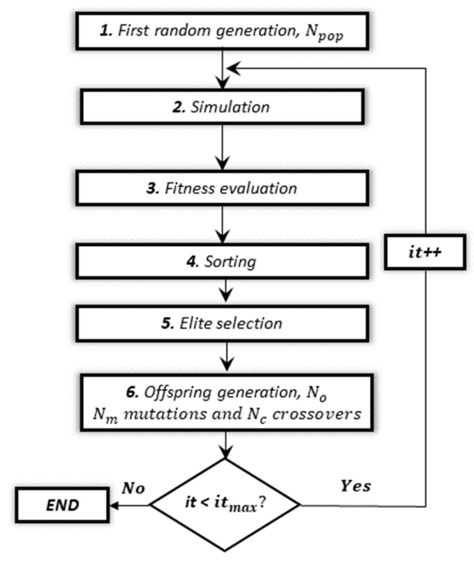
The Genetic Algorithm (GA) used to solve the problem evolves a population of possible solutions (individuals) by means of iterations. An elite group, with the fittest solutions, survives from one generation to the next while the process is moving forward using Cm as the genome of the individuals. Additionally, crossover and mutation operators are applied to generate and offspring of individuals from the elite group at each iteration. The fuzzy optimisation algorithm is the procedure for the calculation of the driving commands when the fuzzy parameters are included. The GA-F process is graphically described in Figure 6 and it is explained as follows:
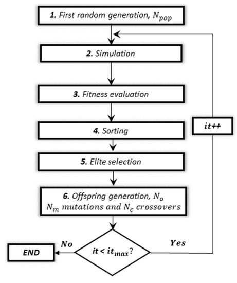
Figure 6.
Flowchart of the GA.
- First random generation of individuals (Cm) equal to the population size Npop.
- Simulation of command matrix of the population. This step generates a running time and an energy consumption associated to each individual.
- Evaluation of each individual by the fitness function (Equation (29)).
- Sorting of each individual in increasing order by means of their fitness value.
- Elite group selection. The first individuals Ne survive in the next iteration population and the rest are eliminated.
- Offspring generation. Mutation and crossover operators are applied to the elite group to generate new individuals until the population reaches its size Npop. In this step, a number of mutations Nm and a number of crossovers Nc are applied.
- The process is repeated from step 2 until the iteration number (it) is equal to the maximum numbers of iterations defined (itmax), giving the best solution to the fittest in the last population.
The proposed algorithm can be expressed in terms of the α-cuts of the fuzzy numbers [96]. As shown in Figure 4, if the punctuality requirement is expressed as a necessity measure np, the upper limit of the α-cuts of the fuzzy running time (equivalent to the upper limit of the α-cuts of the fuzzy running time) is necessary for the evaluation of the punctuality constraint. For this upper limit to be obtained, given the fuzzy numbers associated with the climatological parameters, it has to be analysed whether the running time is an increasing or a decreasing function in each of them.
As discussed in the model, the running time and energy consumption are dependent on the running resistance model. The running resistance force is a function of the fuzzy parameters introduced in this model: the air density and the wind during operation. In turn, the density is a function of the pressure and the temperature. The wind has been modelled by its intensity or speed and their angle of incidence related to the train’s movement.
With equal , train and railway track data, the running time calculated is a function of the uncertainties considered: pressure (), temperature (), velocity of the wind (), and angle of incidence of the wind (). All climatological factors, running time, and energy consumption are defined as fuzzy parameters.
Function (Equation (30)) is monotonous with all climatological parameters. The greater the running resistance, the lower the acceleration and the greater the running time as a result. In that sense, function is increasing with the air density, and thus, according to Equation (18), it is monotonically increasing with the pressure () and monotonically decreasing with the temperature ().
Regarding the angle of incidence of the wind (), it is necessary to analyse every division of the railway line (explained at the end of Section 2.2). In this case, and taking Figure 1 as a reference, is defined differently depending on the situation. Moreover, the presence of the angle of incidence in Equation (22) has to be considered in order to analyse the behaviour of the function . In this way, the variation of the angle and, therefore, the change of in the term of Equation (22) determines the different situations in the high-speed railway scenario. If the angle of incidence lies between:
- (1)
- then is monotonically decreasing with the angle .
- (2)
- then is monotonically increasing with the angle .
After considering the term of the angle of incidence, the speed is another factor related to the wind and its contribution to the railway operation. Considering Figure 1, the behaviour is as follows:
- (1)
- or then is monotonically increasing with the velocity of the wind.
- (2)
- then is monotonically decreasing with the velocity of the wind.
Likewise, the energy consumption associated to the railway operation is also a function of the climatological parameters:
Function F2 (Equation (31)) is monotonous with all climatological parameters as F1 which permits the application of α-cut calculations. Moreover, the dependence of with these parameters is the same as F1 because the greater the running resistance, the greater the traction effort and energy consumption.
In conclusion, the upper and lower limits of α-cuts, and the upper and lower limits of α-cuts can be calculated by means of the alfa-cut of the parameters. Equations (32)–(39) show the corresponding formulas for the 4 quadrants of the angle of incidence as follows, considering the situations presented previously:
• For :
• For :
• For :
• For :
Figure 7 shows an example corresponding to the case of how the climatological fuzzy parameters are considered and the results associated with a specific necessity level of punctuality.

Figure 7.
Climatological fuzzy parameters and fuzzy results.
Therefore, the proposed problem can be solved with the application of the GA-F by means of α-cuts with α = 1 − np. The parameter np is the imposed punctuality constraint. The algorithm will search for the solution in the form of a Command Matrix with a fuzzy running time associated. Its upper α-cut gives the objective running time as a result, considering punctuality requirements and minimising the energy consumption.
5. Case Study
5.1. Introduction
Real commercial service and infrastructure data of a Spanish high-speed railway line have been analysed in this paper. The railway line is operated by a train with an unladen mass of 322 t, a length of 200 m, a maximum traction effort of 200 kN, and a maximum speed of 300 km/h.
This line has been divided as shown in the following figures to elaborate an appropriate data analysis as explained at the end of Section 2.2. The railway line has been divided into zones where the wind is considered constant as can be seen in Figure 8a, and into sections where the angle of the track (Table 1) is considered constant as shown in Figure 8b.

Figure 8.
(a) Wind zones; (b) Constant trip directions zones.

Table 1.
Angle of the railway track.
5.2. Fuzzy Climatological Parameters
The climatological parameters have been modelled taking into account the temperature, the wind intensity, and its angle of incidence collected by the State Meteorological Agency of the Spanish Government [97] in every one of the closest weather stations to the railway line for this case study, and the pressure is a function of the track altitude according to the International Standard Atmosphere [87].
The following tables collect the fuzzy climatological numbers modelled: temperature, pressure, intensity, and angle of incidence of the wind (Table 2, Table 3, Table 4 and Table 5, respectively).

Table 2.
Fuzzy temperature, .

Table 3.
Fuzzy pressure, .

Table 4.
Fuzzy intensity of the wind, .

Table 5.
Fuzzy angle of incidence of the wind, .
5.3. Results
5.3.1. Flat-Out Driving
Initially, the flat-out driving simulations are presented for the Initial Case scenario, with no climatological parameters, and also for the scenarios when the climatological parameters are considered (both in winter and summer). The flat-out driving is the fastest possible in the journey fulfiling the speed limitations of the line. This type of driving has the fastest running time and the associated highest energy consumption.
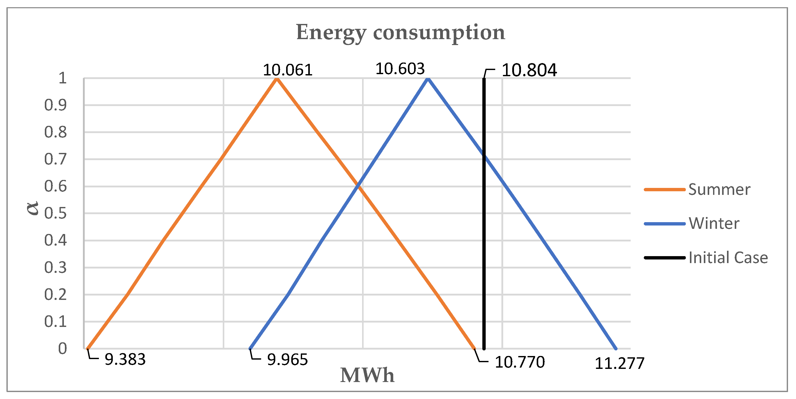
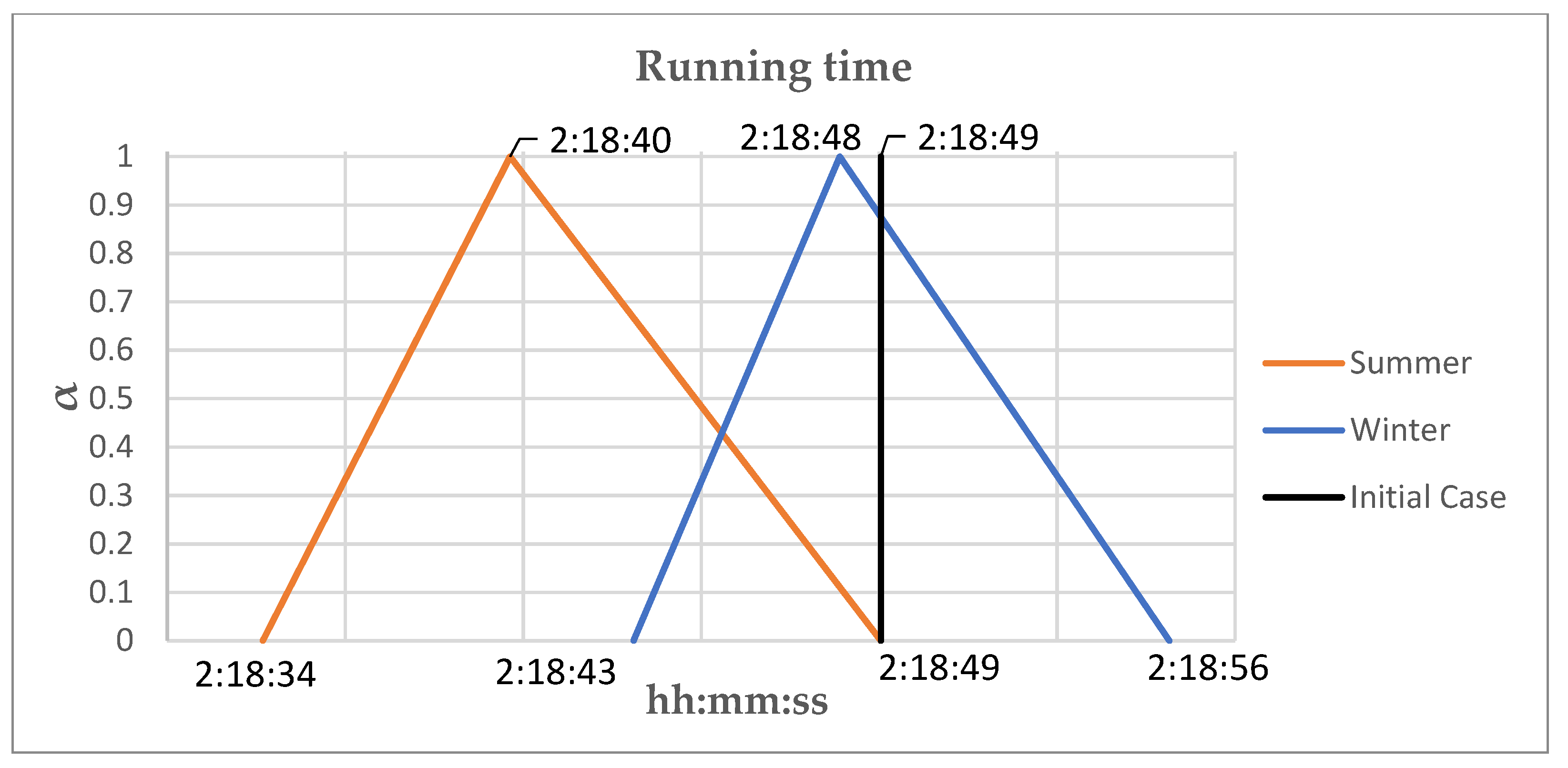
The running time in the simulated Initial Case (no climatological parameters) is 2:18:49, and the associated energy consumption is 10.804 MWh. Table 6 presents the results.

Table 6.
Flat-out driving results.
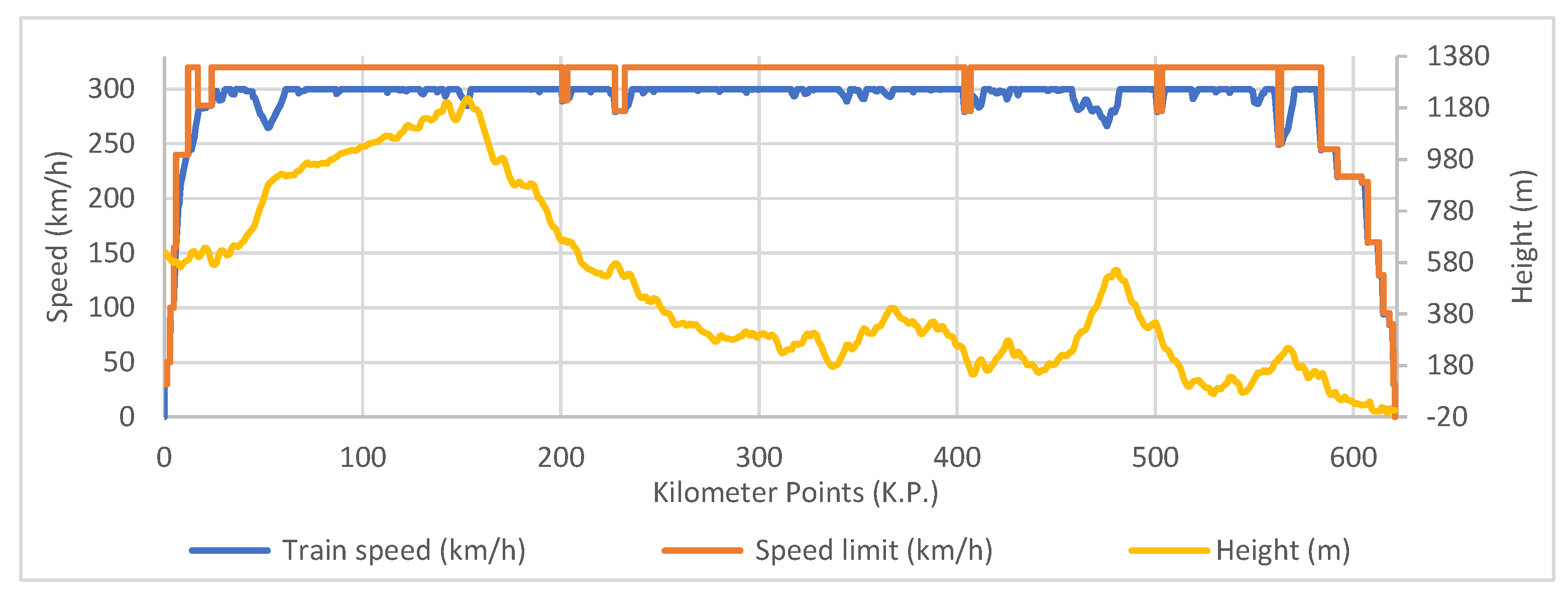
Figure 9 shows the speed profile of the train for the Initial Case, when the flat-out driving is applied and climatological parameters are not impacting the operation.
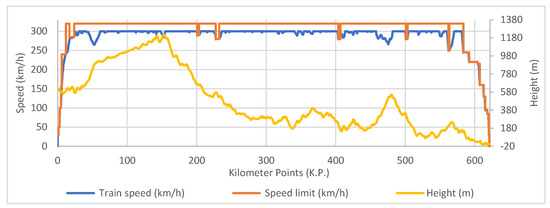
Figure 9.
Flat-out speed profile.
The running time and the energy consumption shown in Table 6 for winter and summer climatological conditions, correspond to the value calculated for the core of the fuzzy sets of temperature, pressure, wind intensity, and angle of incidence.
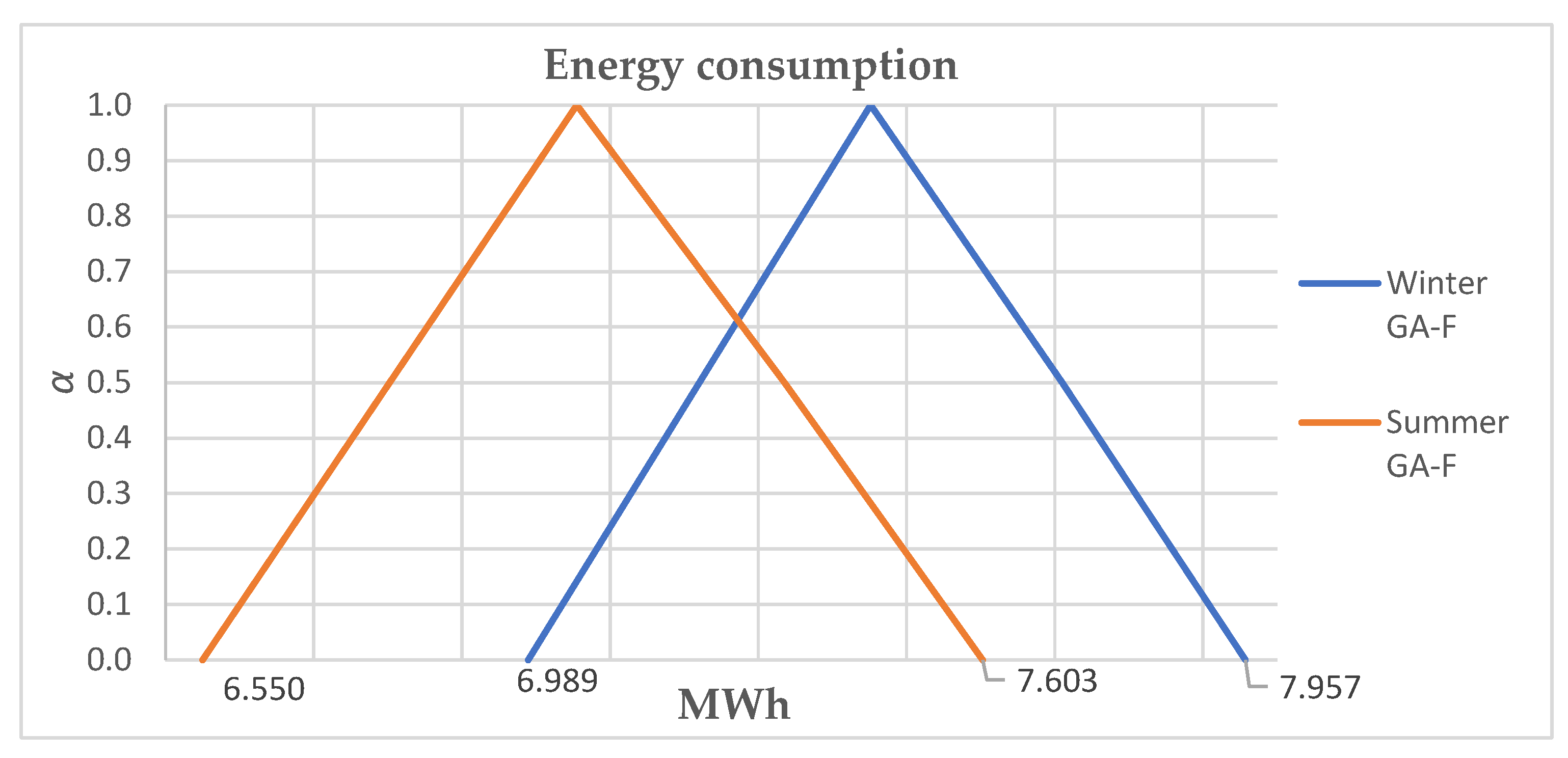
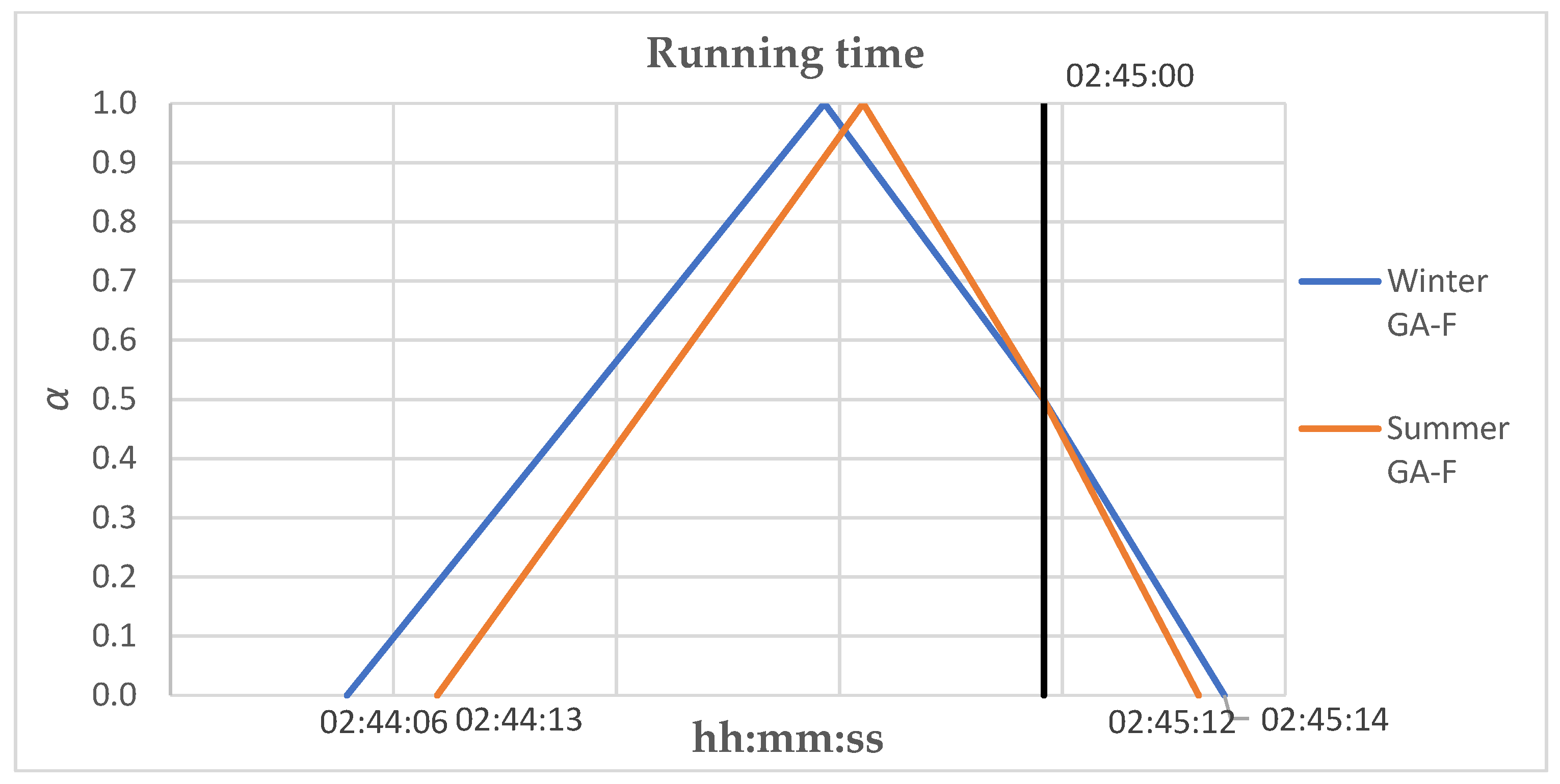
Figure 10 and Figure 11 show the energy consumption of the flat-out driving and the associated running time when the uncertainty in the climatological parameters are included.
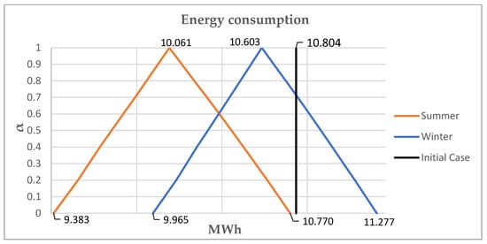
Figure 10.
Fuzzy energy consumption applying flat-out driving.
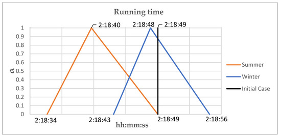
Figure 11.
Fuzzy running time applying flat-out driving.
The impact of climatological parameters on energy consumption is more important than on the running time. In the summer scenario shown in Figure 10, the variation of energy consumption for the minimum and maximum values (support of the fuzzy numbers) is 14.8% in summer and 13.2% in winter. To analyse the impact of winter and summer conditions on the energy consumption, the core of the fuzzy energy consumption in summer and winter can be compared; this comparison shows that the energy consumption is 5.4% less in summer than in winter.
On the other hand, the impact on the running times is less significant. In summer, the variation is 0.18%, and 0.16% in winter. The variation between summer and winter conditions shows a difference of 0.1%.
5.3.2. Eco-Driving Design without Climatological Parameters
After analysing the impact of weather conditions on the flat-out driving, the driving optimisation model is run to design the eco-driving without taking into account the weather conditions, which is solved by means of a GA. This would be the typical approach to solving the problem and will serve as a basis for comparison with the model proposed in this article. The objective travel time for the journey is 2 h and 45 min.
The result of the optimisation is the Command Matrix to apply to obtain the optimal driving, shown in Table 7.

Table 7.
Command Matrix.
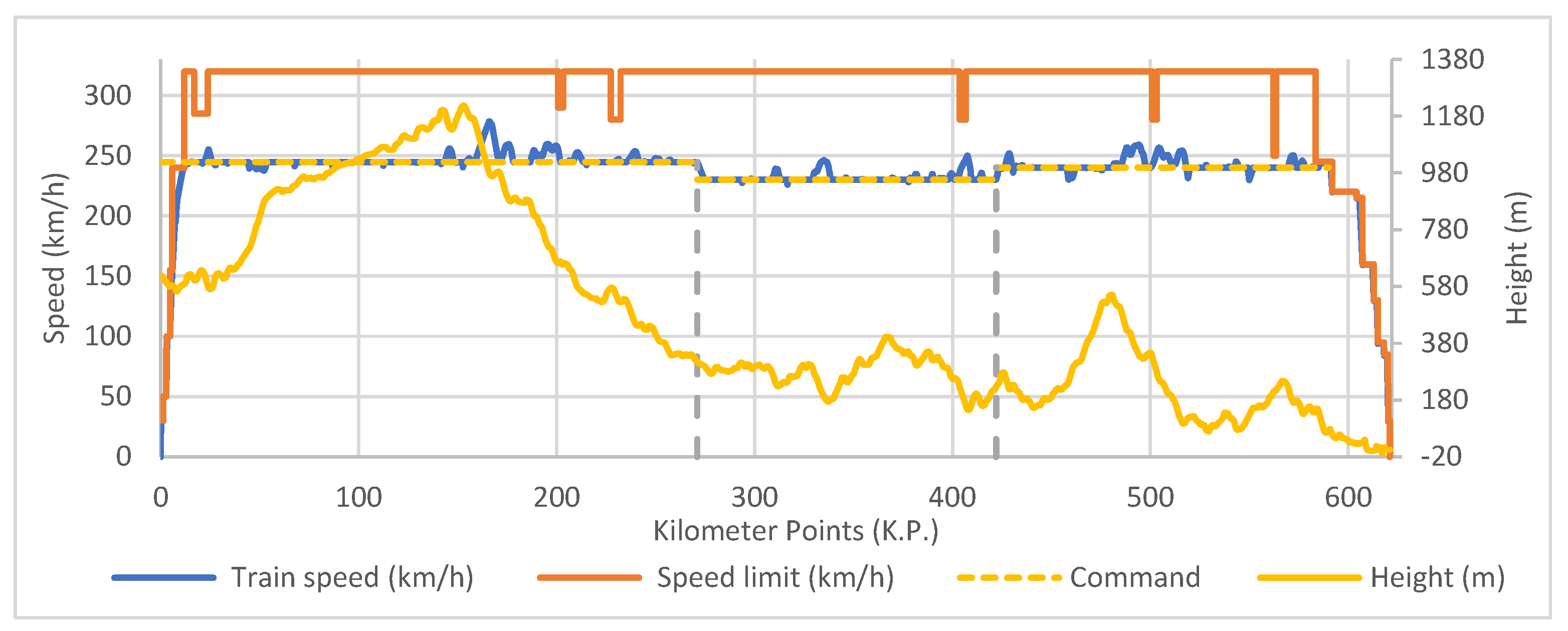
Figure 12 shows the speed profile for the eco-driving obtained from the optimisation model. The driving commands produce the nominal driving and define the commercial eco-driving designed in a specific railway operation. This driving produces an energy consumption of 7.589 MWh.
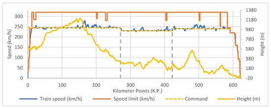
Figure 12.
Eco-driving speed profile.
In Table 8, the energy consumption obtained by the eco-driving design and the associated energy saving compared to the flat-out driving can be seen. Thus, following this typical procedure, the energy saving that the railway operator would expect would be 29.76%. The substantial and significant energy saving is achieved due to the slack time included in the timetable (necessary to satisfy punctuality when a delay arises), and due to the eco-driving design to use the slack time optimally to minimise the energy consumption. Other studies show similar energy savings, 31.27% in [16] and 35.54% in [35].

Table 8.
Energy savings with no weather conditions.
5.3.3. Eco-Driving with Fuzzy Climatological Parameters Applying GA-F
The next step is the execution of the proposed GA-F model to optimise the driving considering the fuzzy climatological parameters (Table 2, Table 3, Table 4 and Table 5) with an objective running time of 2:45:00. The punctuality constraint is expressed as a necessity measure . The fuzzy optimisation model has been applied for the summer and winter scenarios.
Table 9 collects the results (energy consumption and running time) obtained by simulating for different α-cut with the eco-driving commands obtained with the optimisation model. Specifically, the lower and upper limits of the α-cuts with α = 0 and with α = 0.5 are shown, as well as the core (α = 1).

Table 9.
Fuzzy results obtained with the eco-driving design applying GA-F with np = 0.5 in winter and in summer.
For the fuzzy energy consumption results, the difference between the core values in summer and winter is 5.32%. The variation between the lower limit of α-cut = 0 and the upper limit of α-cut = 0 in winter is 12.16% and 13.85% in summer. On the other hand, the variation related to the running time is 00:01:08 hh:mm:ss for the winter scenario (0.69%) and 0:00:59 for the summer scenario (0.60%).
Figure 13 and Figure 14 are the fuzzy energy consumption and the fuzzy running times obtained by applying the proposed GA-F model with fuzzy climatological parameters. Figure 14 shows that the objective running time is achieved when as the necessity measure for punctuality imposed was np = 0.5 = 1 −.
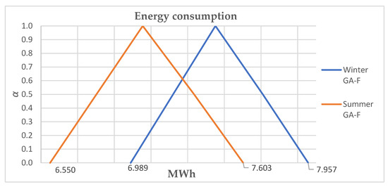
Figure 13.
Fuzzy energy consumption applying GA-F with np = 0.5 in winter and in summer.

Figure 14.
Fuzzy running time applying GA-F with np = 0.5 in winter and in summer.
To conclude, the typical eco-driving design procedure where weather conditions are not considered would provide expected energy savings of 29.76%, as previously indicated. With the application of the proposed GA-F model with fuzzy climatological parameters, the energy consumption of the new eco-driving designs is lower, and thus, the expected energy savings are higher (34.7% in summer and 31.03% in winter). Weather conditions have a significant impact on energy consumption and to a lesser extent, on journey time, and it is worth incorporating this information into the model in order to adapt driving to these pressure, temperature, and wind conditions on the journey under analysis.
6. Conclusions
This paper proposes a new model to design eco-driving in railway lines taking into account climatological conditions. The climatological parameters affecting the model are the temperature, pressure, the wind intensity, and its angle of incidence. The uncertainty associated with these climatological parameters is modelled by fuzzy numbers, and the optimisation problem is solved by means of a GA-F, Genetic Algorithm with fuzzy parameters. The analysis of the energy consumption and running time functions depending on these parameters permits an efficient calculation and resolution of the problem applying α-cut simulations.
The proposed model has been applied to a real Spanish high-speed railway line. First, the flat-out driving has been simulated and the important impact that the climatological parameters have on the energy consumption of the train and to a lesser extent on the running times have been shown.
Then, the efficient driving is designed without and with climatological parameters (applying the proposed GA-F). The eco-driving design is based on applying coasting commands and speed regulation without braking commands. In this case study, it has been shown that the expected energy savings obtained in this process are underestimated when eco-driving is designed without considering climatological parameters. Of course, depending on the specific characteristics of the railway line under study, the climatological conditions could be less or more favorable. However, it can be concluded that weather conditions have a significant impact on energy consumption and to a lesser extent, on journey time, and it is worth incorporating this information into the model in order to adapt driving to the pressure, temperature, and wind conditions on the journey under analysis. The final aim is to maximise energy savings considering as much as possible parameterised data involved in the rail traffic operations.
Future developments will be oriented to the application of the model in real-time to adapt the optimal driving to the current climatological conditions and include other sources of uncertainty related to the traffic conditions.
Author Contributions
Software, M.B.-C. and A.F.-R.; writing, M.B.-C.; investigation, M.B.-C., A.F.-R., A.F.-C. and A.P.C.; validation, A.F.-R., A.F.-C. and A.P.C.; Conceptualization, A.F.-C. and A.P.C. All authors have read and agreed to the published version of the manuscript.
Funding
This research received no external funding.
Institutional Review Board Statement
Not applicable.
Informed Consent Statement
Not applicable.
Data Availability Statement
Not applicable.
Conflicts of Interest
The authors declare no conflict of interest.
References
- Liu, R.; Golovitcher, I.M. Energy-Efficient Operation of Rail Vehicles. Transp. Res. Part A Policy Pract. 2003, 37, 917–932. [Google Scholar] [CrossRef]
- Lechelle, S.A.; Mouneimne, Z.S. OptiDrive: A Practical Approach for the Calculation of Energy-Optimised Operating Speed Profiles. In Proceedings of the IET Conference on Railway Traction Systems (RTS 2010), Birmingham, UK, 13–15 April 2010; pp. 1–8. [Google Scholar]
- Feng, X.; Zhang, H.; Ding, Y.; Liu, Z.; Peng, H.; Xu, B. A Review Study on Traction Energy Saving of Rail Transport. Discret. Dyn. Nat. Soc. 2013, 2013, e156548. [Google Scholar] [CrossRef]
- Koseki, T. Technologies for Saving Energy in Railway Operation: General Discussion on Energy Issues Concerning Railway Technology. IEEJ Trans. Electr. Electron. Eng. 2010, 5, 285–290. [Google Scholar] [CrossRef]
- Zhou, W.; Fan, W.; You, X.; Deng, L. Demand-Oriented Train Timetabling Integrated with Passenger Train-Booking Decisions. Sustainability 2019, 11, 4932. [Google Scholar] [CrossRef] [Green Version]
- Zhou, W.; You, X.; Fan, W. A Mixed Integer Linear Programming Method for Simultaneous Multi-Periodic Train Timetabling and Routing on a High-Speed Rail Network. Sustainability 2020, 12, 1131. [Google Scholar] [CrossRef] [Green Version]
- Zhou, W.; Oldache, M. Integrated Optimization of Line Planning, Timetabling and Rolling Stock Allocation for Urban Railway Lines. Sustainability 2021, 13, 13059. [Google Scholar] [CrossRef]
- Abril, M.; Salido, M.A.; Barber, F. Distributed Search in Railway Scheduling Problems. Eng. Appl. Artif. Intell. 2008, 21, 744–755. [Google Scholar] [CrossRef] [Green Version]
- Hassannayebi, E.; Zegordi, S.H. Variable and Adaptive Neighbourhood Search Algorithms for Rail Rapid Transit Timetabling Problem. Comput. Oper. Res. 2017, 78, 439–453. [Google Scholar] [CrossRef]
- Peña-Alcaraz, M.; Fernández, A.; Cucala, A.P.; Ramos, A.; Pecharromán, R.R. Optimal Underground Timetable Design Based on Power Flow for Maximizing the Use of Regenerative-Braking Energy. Proc. Inst. Mech. Eng. Part F J. Rail Rapid Transit 2012, 226, 397–408. [Google Scholar] [CrossRef]
- Wang, L.; Qin, Y.; Xu, J.; Jia, L. A Fuzzy Optimization Model for High-Speed Railway Timetable Rescheduling. Discret. Dyn. Nat. Soc. 2012, 2012, e827073. [Google Scholar] [CrossRef]
- Feng, X.; Feng, J.; Wu, K.; Liu, H.; Sun, Q. Evaluating Target Speeds of Passenger Trains in China for Energy Saving in the Effect of Different Formation Scales and Traction Capacities. Int. J. Electr. Power Energy Syst. 2012, 42, 621–626. [Google Scholar] [CrossRef]
- Howlett, P.G.; Milroy, I.P.; Pudney, P.J. Energy-Efficient Train Control. Control Eng. Pract. 1994, 2, 193–200. [Google Scholar] [CrossRef]
- Jong, J.-C.; Chang, S. Algorithms for Generating Train Speed Profiles. J. East. Asia Soc. Transp. Stud. 2005, 6, 356–371. [Google Scholar]
- Howlett, P. Optimal Strategies for the Control of a Train. Automatica 1996, 32, 519–532. [Google Scholar] [CrossRef]
- Bocharnikov, Y.V.; Tobias, A.M.; Roberts, C.; Hillmansen, S.; Goodman, C.J. Optimal Driving Strategy for Traction Energy Saving on DC Suburban Railways. IET Electr. Power Appl. 2007, 1, 675–682. [Google Scholar] [CrossRef]
- Domínguez, M.; Fernández, A.; Cucala, A.P.; Lukaszewicz, P. Optimal Design of Metro Automatic Train Operation Speed Profiles for Reducing Energy Consumption. Proc. Inst. Mech. Eng. Part F J. Rail Rapid Transit 2011, 225, 463–474. [Google Scholar] [CrossRef]
- Ichikawa, K. Application of Optimization Theory for Bounded State Variable Problems to the Operation of Train. Bull. JSME 1968, 11, 857–865. [Google Scholar] [CrossRef]
- Chang, C.S.; Sim, S.S. Optimising Train Movements through Coast Control Using Genetic Algorithms. IEE Proc.-Electr. Power Appl. 1997, 144, 65–73. [Google Scholar] [CrossRef]
- Golovitcher, I.M. Energy Efficient Control of Rail Vehicles. In Proceedings of the 2001 IEEE International Conference on Systems, Man and Cybernetics, Tucson, AZ, USA, 7–10 October 2001; e-Systems and e-Man for Cybernetics in Cyberspace (Cat.No.01CH37236). Volume 1, pp. 658–663. [Google Scholar]
- Howlett, P.G.; Pudney, P.J.; Vu, X. Local Energy Minimization in Optimal Train Control. Automatica 2009, 45, 2692–2698. [Google Scholar] [CrossRef]
- Coleman, D.; Howlett, P.; Pudney, P.; Vu, X.; Yee, R. Coasting Boards vs Optimal Control. In Proceedings of the IET Conference on Railway Traction Systems (RTS 2010), Birmingham, UK, 13–15 April 2010; pp. 1–5. [Google Scholar]
- Hwang, H.-S. Control Strategy for Optimal Compromise between Trip Time and Energy Consumption in a High-Speed Railway. IEEE Trans. Syst. Man Cybern.-Part A Syst. Hum. 1998, 28, 791–802. [Google Scholar] [CrossRef]
- Sicre, C.; Cucala, A.P.; Fernández, A.; Lukaszewicz, P. Modeling and Optimizing Energy-Efficient Manual Driving on High-Speed Lines. IEEJ Trans. Electr. Electron. Eng. 2012, 7, 633–640. [Google Scholar] [CrossRef]
- Yang, X.; Chen, A.; Ning, B.; Tang, T. Measuring Route Diversity for Urban Rail Transit Networks: A Case Study of the Beijing Metro Network. IEEE Trans. Intell. Transp. Syst. 2017, 18, 259–268. [Google Scholar] [CrossRef]
- Albrecht, T.; Binder, A.; Gassel, C. Applications of Real-Time Speed Control in Rail-Bound Public Transportation Systems. IET Intell. Transp. Syst. 2013, 7, 305–314. [Google Scholar] [CrossRef]
- Lu, S.; Hillmansen, S.; Ho, T.K.; Roberts, C. Single-Train Trajectory Optimization. IEEE Trans. Intell. Transp. Syst. 2013, 14, 743–750. [Google Scholar] [CrossRef]
- Miyatake, M.; Ko, H. Optimization of Train Speed Profile for Minimum Energy Consumption. IEEJ Trans. Electr. Electron. Eng. 2010, 5, 263–269. [Google Scholar] [CrossRef]
- Miyatake, M.; Matsuda, K. Energy Saving Speed and Charge/Discharge Control of a Railway Vehicle with On-Board Energy Storage by Means of an Optimization Model. IEEJ Trans. Electr. Electron. Eng. 2009, 4, 771–778. [Google Scholar] [CrossRef]
- Khmelnitsky, E. On an Optimal Control Problem of Train Operation. IEEE Trans. Autom. Control 2000, 45, 1257–1266. [Google Scholar] [CrossRef]
- Yang, J.; Quan, J.; Yan, B.; He, C. Urban Rail Investment and Transit-Oriented Development in Beijing: Can It Reach a Higher Potential? Transp. Res. Part A Policy Pract. 2016, 89, 140–150. [Google Scholar] [CrossRef]
- Gu, Q.; Tang, T.; Cao, F.; Song, Y. Energy-Efficient Train Operation in Urban Rail Transit Using Real-Time Traffic Information. IEEE Trans. Intell. Transp. Syst. 2014, 15, 1216–1233. [Google Scholar] [CrossRef]
- Rodrigo, E.; Tapia, S.; Mera, J.M.; Soler, M. Optimizing Electric Rail Energy Consumption Using the Lagrange Multiplier Technique. J. Transp. Eng. 2013, 139, 321–329. [Google Scholar] [CrossRef]
- Wang, Y.; De Schutter, B.; van den Boom, T.J.J.; Ning, B.; Tang, T. Efficient Bilevel Approach for Urban Rail Transit Operation With Stop-Skipping. IEEE Trans. Intell. Transp. Syst. 2014, 15, 2658–2670. [Google Scholar] [CrossRef]
- Açıkbaş, S.; Söylemez, M. Coasting Point Optimisation for Mass Rail Transit Lines Using Artificial Neural Networks and Genetic Algorithms. Electr. Power Appl. IET 2008, 2, 172–182. [Google Scholar] [CrossRef]
- Chuang, H.-J.; Chen, C.-S.; Lin, C.-H.; Hsieh, C.-H.; Ho, C.-Y. Design of Optimal Coasting Speed for MRT Systems Using ANN Models. IEEE Trans. Ind. Appl. 2009, 45, 2090–2097. [Google Scholar] [CrossRef]
- Koper, E.; Kochan, A. Testing the Smooth Driving of a Train Using a Neural Network. Sustainability 2020, 12, 4622. [Google Scholar] [CrossRef]
- Bocharnikov, Y.V.; Tobias, A.M.; Roberts, C. Reduction of Train and Net Energy Consumption Using Genetic Algorithms for Trajectory Optimisation. In Proceedings of the IET Conference on Railway Traction Systems (RTS 2010), Birmingham, UK, 13–15 April 2010; pp. 1–5. [Google Scholar]
- Li, X.; Lo, H.K. An Energy-efficient Scheduling and Speed Control Approach for Metro Rail Operations. Transp. Res. Part B Methodol. 2014, 64, 73–89. [Google Scholar] [CrossRef]
- Wong, K.K.; Ho, T.K. Coast Control of Train Movement with Genetic Algorithm. In Proceedings of the The 2003 Congress on Evolutionary Computation, Canberra, Australia, 8–12 December 2003; CEC ’03. Volume 2, pp. 1280–1287. [Google Scholar]
- Wong, K.K.; Ho, T.K. Coast Control for Mass Rapid Transit Railways with Searching Methods. IEE Proc.-Electr. Power Appl. 2004, 151, 365–376. [Google Scholar] [CrossRef] [Green Version]
- Yang, L.; Li, K.; Gao, Z.; Li, X. Optimizing Trains Movement on a Railway Network. Omega 2012, 40, 619–633. [Google Scholar] [CrossRef]
- Huang, Y.; Ma, X.; Su, S.; Tang, T. Optimization of Train Operation in Multiple Interstations with Multi-Population Genetic Algorithm. Energies 2015, 8, 14311–14329. [Google Scholar] [CrossRef]
- Wei, L.; Qunzhan, L.; Bing, T. Energy Saving Train Control for Urban Railway Train with Multi-Population Genetic Algorithm. In Proceedings of the 2009 International Forum on Information Technology and Applications, Chengdu, China, 15–17 May 2009; Volume 2, pp. 58–62. [Google Scholar]
- Sicre, C.; Cucala, A.P.; Fernández-Cardador, A. Real Time Regulation of Efficient Driving of High Speed Trains Based on a Genetic Algorithm and a Fuzzy Model of Manual Driving. Eng. Appl. Artif. Intell. 2014, 29, 79–92. [Google Scholar] [CrossRef]
- Cucala, A.P.; Fernández, A.; Sicre, C.; Domínguez, M. Fuzzy Optimal Schedule of High Speed Train Operation to Minimize Energy Consumption with Uncertain Delays and Driver’s Behavioral Response. Eng. Appl. Artif. Intell. 2012, 25, 1548–1557. [Google Scholar] [CrossRef]
- De Cuadra, F. Energy-Saving Automatic Optimisation of Train Speed Commands Using Direct Search Techniques. Comput. Railw. V 1996, 1, 20. [Google Scholar]
- Zhao, N.; Roberts, C.; Hillmansen, S.; Tian, Z.; Weston, P.; Chen, L. An Integrated Metro Operation Optimization to Minimize Energy Consumption. Transp. Res. Part C Emerg. Technol. 2017, 75, 168–182. [Google Scholar] [CrossRef] [Green Version]
- Tian, Z.; Weston, P.; Zhao, N.; Hillmansen, S.; Roberts, C.; Chen, L. System Energy Optimisation Strategies for Metros with Regeneration. World Transit Res. 2017, 75, 120–135. [Google Scholar] [CrossRef]
- Operating Speed Pattern Optimization of Railway Vehicles with Differential Evolution Algorithm|SpringerLink. Available online: https://link.springer.com/article/10.1007/s12239-013-0099-7 (accessed on 8 June 2022).
- Keskin, K.; Karamancioglu, A. Energy-Efficient Train Operation Using Nature-Inspired Algorithms. J. Adv. Transp. 2017, 2017, 6173795. [Google Scholar] [CrossRef] [Green Version]
- Xie, T.; Wang, S.; Zhao, X.; Zhang, Q. Optimization of Train Energy-Efficient Operation Using Simulated Annealing Algorithm. In Proceedings of the Intelligent Computing for Sustainable Energy and Environment; Li, K., Li, S., Li, D., Niu, Q., Eds.; Springer: Berlin/Heidelberg, Germany, 2013; pp. 351–359. [Google Scholar]
- Chevrier, R.; Pellegrini, P.; Rodriguez, J. Energy Saving in Railway Timetabling: A Bi-Objective Evolutionary Approach for Computing Alternative Running Times. Transp. Res. Part C Emerg. Technol. 2013, 37, 20–41. [Google Scholar] [CrossRef] [Green Version]
- Carvajal-Carreño, W.; Cucala, A.P.; Fernández-Cardador, A. Optimal Design of Energy-Efficient ATO CBTC Driving for Metro Lines Based on NSGA-II with Fuzzy Parameters. Eng. Appl. Artif. Intell. 2014, 36, 164–177. [Google Scholar] [CrossRef]
- Domínguez, M.; Fernández-Cardador, A.; Cucala, A.P.; Gonsalves, T.; Fernández, A. Multi Objective Particle Swarm Optimization Algorithm for the Design of Efficient ATO Speed Profiles in Metro Lines. Eng. Appl. Artif. Intell. 2014, 29, 43–53. [Google Scholar] [CrossRef]
- Ke, B.; Lin, C.; Yang, C. Optimisation of train energy-efficient operation for mass rapid transit systems. IET Intell. Transp. Syst. 2012, 6, 58–66. [Google Scholar] [CrossRef]
- Fernandez-Rodriguez, A.; Fernandez-Cardador, A.; Cucala, A.P.; Dominguez, M.; Gonsalves, T. Design of Robust and Energy-Efficient ATO Speed Profiles of Metropolitan Lines Considering Train Load Variations and Delays. IEEE Trans. Intell. Transport. Syst. 2015, 16, 2061–2071. [Google Scholar] [CrossRef] [Green Version]
- Wang, P.; Goverde, R.M.P. Multi-Train Trajectory Optimization for Energy Efficiency and Delay Recovery on Single-Track Railway Lines. Transp. Res. Part B: Methodol. 2017, 105, 340–361. [Google Scholar] [CrossRef]
- Fernández-Rodríguez, A.; Fernández-Cardador, A.; Cucala, A.P. Balancing Energy Consumption and Risk of Delay in High Speed Trains: A Three-Objective Real-Time Eco-Driving Algorithm with Fuzzy Parameters. Transp. Res. Part C Emerg. Technol. 2018, 95, 652–678. [Google Scholar] [CrossRef]
- Kloow, L.; Jenstav, M. High-Speed Train Operation in Winter Climate; Transrail Publication BVF5; KTH Railway Group: Stockholm, Sweden, 2011; Volume 2, ISBN 978-91-7501-121-9. [Google Scholar]
- Wang, J.; Granlöf, M.; Yu, J. Effects of Winter Climate on Delays of High Speed Passenger Trains in Botnia-Atlantica Region. J. Rail Transp. Plan. Manag. 2021, 18, 100251. [Google Scholar] [CrossRef]
- Huang, P.; Wen, C.; Fu, L.; Lessan, J.; Jiang, C.; Peng, Q.; Xu, X. Modeling Train Operation as Sequences: A Study of Delay Prediction with Operation and Weather Data. Transp. Res. Part E Logist. Transp. Rev. 2020, 141, 102022. [Google Scholar] [CrossRef]
- Zakeri, G.; Olsson, N.O.E. Investigating the Effect of Weather on Punctuality of Norwegian Railways: A Case Study of the Nordland Line. J. Mod. Transport. 2018, 26, 255–267. [Google Scholar] [CrossRef] [Green Version]
- Ling, X.; Peng, Y.; Sun, S.; Li, P.; Wang, P. Uncovering Correlation between Train Delay and Train Exposure to Bad Weather. Phys. A Stat. Mech. Its Appl. 2018, 512, 1152–1159. [Google Scholar] [CrossRef]
- Zhang, J.; Ye, Y.; Zhou, Y. A Hybrid Forewarning Algorithm for Train Operation under Adverse Weather Conditions. In Proceedings of the RailNorrköping 2019, 8th International Conference on Railway Operations Modelling and Analysis (ICROMA), Norrköping, Sweden, 17–20 June 2019. [Google Scholar]
- Dindar, S.; Kaewunruen, S.; An, M.; Sussman, J.M. Bayesian Network-Based Probability Analysis of Train Derailments Caused by Various Extreme Weather Patterns on Railway Turnouts. Saf. Sci. 2018, 110, 20–30. [Google Scholar] [CrossRef] [Green Version]
- Ludvigsen, J.; Klæboe, R. Extreme Weather Impacts on Freight Railways in Europe. Nat. Hazards 2014, 70, 767–787. [Google Scholar] [CrossRef]
- Xia, Y.; Van Ommeren, J.N.; Rietveld, P.; Verhagen, W. Railway Infrastructure Disturbances and Train Operator Performance: The Role of Weather. Transp. Res. Part D Transp. Environ. 2013, 18, 97–102. [Google Scholar] [CrossRef]
- Wei, D.; Liu, H.; Qin, Y. Modeling Cascade Dynamics of Railway Networks under Inclement Weather. Transp. Res. Part E Logist. Transp. Rev. 2015, 80, 95–122. [Google Scholar] [CrossRef]
- Bellman, R.E.; Zadeh, L.A. Decision-Making in a Fuzzy Environment. Manag. Sci. 1970, 17, 141–164. [Google Scholar] [CrossRef]
- Tsang, C.-W.; Ho, T.-K. A Prioritized Fuzzy Constraint Satisfaction Approach to Model Agent Negotiation for Railway Scheduling. In Proceedings of the 2004 International Conference on Machine Learning and Cybernetics (IEEE Cat. No.04EX826), Shanghai, China, 26–29 August 2004; Volume 3, pp. 1795–1801. [Google Scholar]
- Chang, C.S.; Thia, B.S. Online Rescheduling of Mass Rapid Transit Systems: Fuzzy Expert System Approach. IEE Proc.-Electr. Power Appl. 1996, 143, 307–316. [Google Scholar] [CrossRef]
- Chang, C.S.; Phoa, Y.H.; Wang, W.; Thia, B.S. Economy/Regularity Fuzzy-Logic Control of DC Railway Systems Using Event-Driven Approach. IEE Proc.-Electr. Power Appl. 1996, 143, 9–17. [Google Scholar] [CrossRef]
- Isaai, M.T.; Kanani, A.; Tootoonchi, M.; Afzali, H.R. Intelligent Timetable Evaluation Using Fuzzy AHP. Expert Syst. Appl. 2011, 38, 3718–3723. [Google Scholar] [CrossRef]
- Yang, L.; Li, K.; Gao, Z. Train Timetable Problem on a Single-Line Railway With Fuzzy Passenger Demand. IEEE Trans. Fuzzy Syst. 2009, 17, 617–629. [Google Scholar] [CrossRef]
- Hanaoka, S.; Kunadhamraks, P. Multiple Criteria and Fuzzy Based Evaluation of Logistics Performance for Intermodal Transportation. J. Adv. Transp. 2009, 43, 123–153. [Google Scholar] [CrossRef]
- Jia, L.-M.; Zhang, X.-D. Distributed Intelligent Railway Traffic Control Based on Fuzzy Decisionmaking. Fuzzy Sets Syst. 1994, 62, 255–265. [Google Scholar] [CrossRef]
- Fay, A. A Fuzzy Knowledge-Based System for Railway Traffic Control. Eng. Appl. Artif. Intell. 2000, 13, 719–729. [Google Scholar] [CrossRef]
- Yasunobu, S.; Miyamoto, S.; Ihara, H. Fuzzy Control for Automatic Train Operation System. IFAC Proc. Vol. 1983, 16, 33–39. [Google Scholar] [CrossRef]
- Chang, C.-S.; Xu, D.Y.; Quek, H.B. Pareto-Optimal Set Based Multiobjective Tuning of Fuzzy Automatic Train Operation for Mass Transit System. IEE Proc.-Electr. Power Appl. 1999, 146, 577–583. [Google Scholar] [CrossRef] [Green Version]
- Saba, E.; Kalwar, I.H.; Unar, M.A.; Memon, A.L.; Pirzada, N. Fuzzy Logic-Based Identification of Railway Wheelset Conicity Using Multiple Model Approach. Sustainability 2021, 13, 10249. [Google Scholar] [CrossRef]
- Blagojević, A.; Kasalica, S.; Stević, Ž.; Tričković, G.; Pavelkić, V. Evaluation of Safety Degree at Railway Crossings in Order to Achieve Sustainable Traffic Management: A Novel Integrated Fuzzy MCDM Model. Sustainability 2021, 13, 832. [Google Scholar] [CrossRef]
- Goodman, C.J.; Siu, L.K.; Ho, T.K. A Review of Simulation Models for Railway Systems. In Proceedings of the 1998 International Conference on Developments in Mass Transit Systems Conf. Publ. No. 453, London, UK, 20–23 April 1998; pp. 80–85. [Google Scholar]
- Law, A.M.; Kelton, W.D. Simulation Modeling and Analysis, 2nd ed.; McGraw-Hill Series in Industrial Engineering and Management Science; McGraw-Hill: New York, NY, USA, 1991; ISBN 978-0-07-036698-5. [Google Scholar]
- Lukaszewicz, P. A Simple Method to Determine Train Running Resistance from Full-Scale Measurements. Proc. Inst. Mech. Eng. Part F J. Rail Rapid Transit 2007, 221, 331–337. [Google Scholar] [CrossRef]
- Davis, W. The Tractive Resistance of Electric Locomotives and Cars; General Electric: Schenectady, NY, USA, 1926. [Google Scholar]
- ISO 2533:1975; Standard Atmosphere. ISO: Geneva, Switzerland, 1975.
- Schetz, J.A. Aerodynamics of high-speed trains. Annu. Rev. Fluid Mech. 2001, 33, 371–414. [Google Scholar] [CrossRef] [Green Version]
- Kwon, H. A Study on the Resistance Force and the Aerodynamic Drag of Korean High-Speed Trains. Veh. Syst. Dyn. 2018, 56, 1250–1268. [Google Scholar] [CrossRef]
- Gawthorpe, R.G. Wind Effects on Ground Transportation. J. Wind Eng. Ind. Aerodyn. 1994, 52, 73–92. [Google Scholar] [CrossRef]
- Peters, J.-L. Bestimmung Des Aerodynamischen Widerstandes Des ICE/V Im Tunnel Und Auf Freier Strecke Durch Auslaufversuche. ETR. Eisenb. Rundsch. 1990, 39, 559–564. [Google Scholar]
- Zadeh, L.A. Fuzzy Sets. Inf. Control 1965, 8, 338–353. [Google Scholar] [CrossRef] [Green Version]
- Xiao, Z.; Xia, S.; Gong, K.; Li, D. The Trapezoidal Fuzzy Soft Set and Its Application in MCDM. Appl. Math. Model. 2012, 36, 5844–5855. [Google Scholar] [CrossRef]
- Chang, C.-T. An Approximation Approach for Representing S-Shaped Membership Functions. IEEE Trans. Fuzzy Syst. 2010, 18, 412–424. [Google Scholar]
- Vasant, P.; Ganesan, T.; Elamvazuthi, I. Improved Tabu Search Recursive Fuzzy Method for Crude Oil Industry. Int. J. Model. Simul. Sci. Comput. 2012, 3, 1150002. [Google Scholar] [CrossRef]
- Chanas, S.; Kołodziejczyk, W.; Machaj, A. A Fuzzy Approach to the Transportation Problem. Fuzzy Sets Syst. 1984, 13, 211–221. [Google Scholar] [CrossRef]
- AEMET OpenData. Available online: https://opendata.aemet.es/centrodedescargas/productosAEMET? (accessed on 3 February 2022).
Publisher’s Note: MDPI stays neutral with regard to jurisdictional claims in published maps and institutional affiliations. |
© 2022 by the authors. Licensee MDPI, Basel, Switzerland. This article is an open access article distributed under the terms and conditions of the Creative Commons Attribution (CC BY) license (https://creativecommons.org/licenses/by/4.0/).


