
Application of Remote-Sensing-Based Hydraulic Model and Hydrological Model in Flood Simulation


Abstract
1. Introduction
2. Materials and Methods
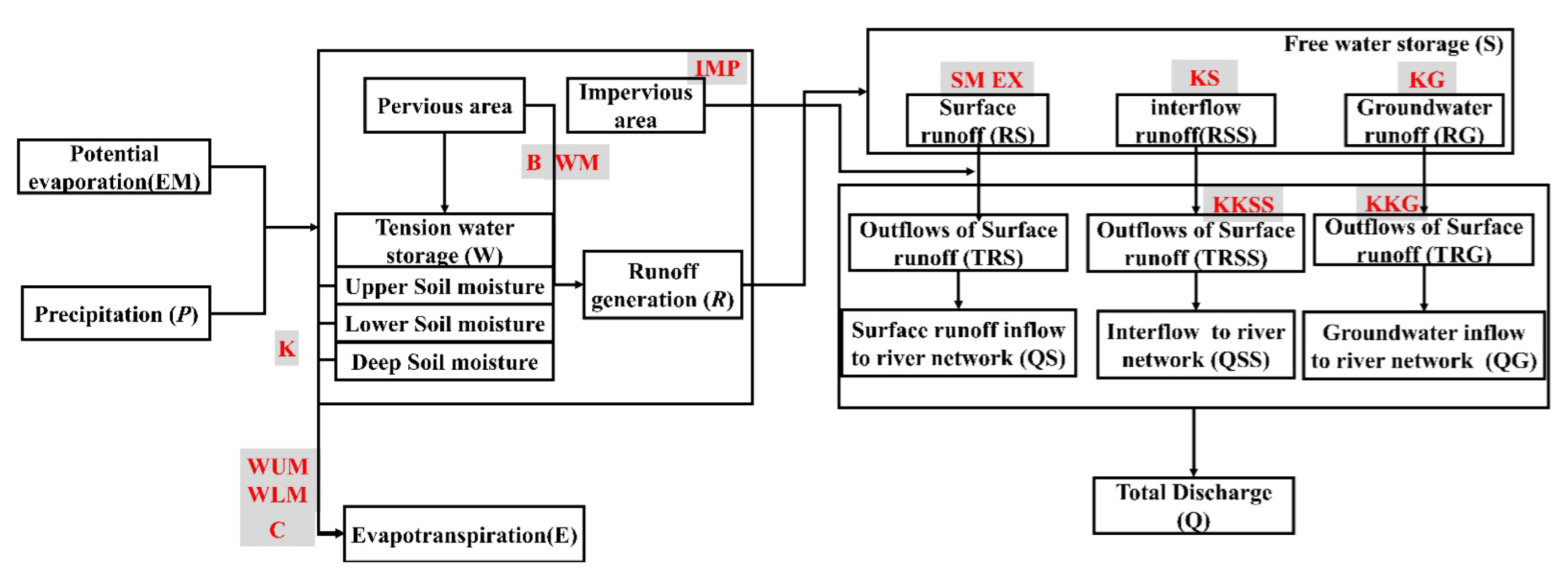
2.1. Hydrological Model (XAJ Model)
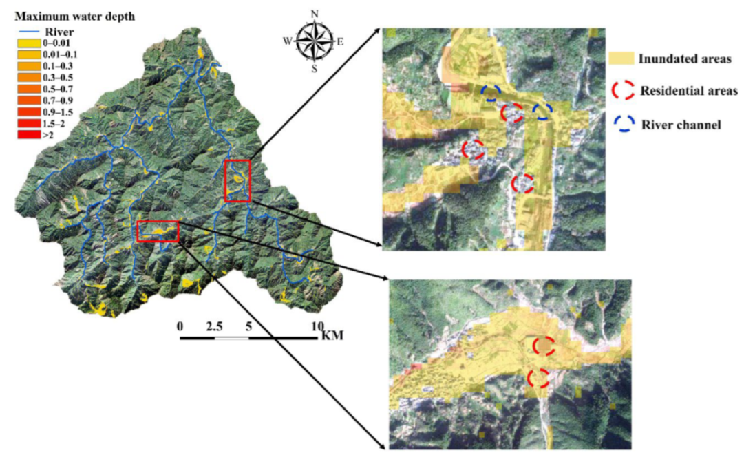
2.2. Two-Dimensional Hydraulic Model (2D Model)
2.3. Study Area and Data Description
2.4. Data Preprocessing and Model Settings
2.5. Modeling Evaluation Criteria
3. Results and Discussion
3.1. Land Use Change in Chengcun Basin
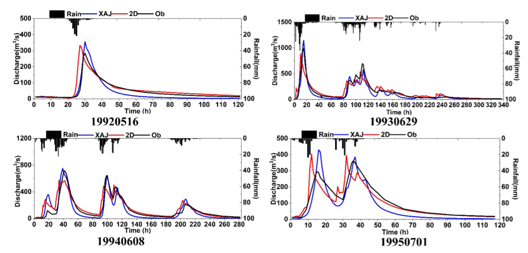
3.2. Comparing the Results of the Hydrological and Hydraulic Models
4. Conclusions
Author Contributions
Funding
Institutional Review Board Statement
Informed Consent Statement
Data Availability Statement
Acknowledgments
Conflicts of Interest
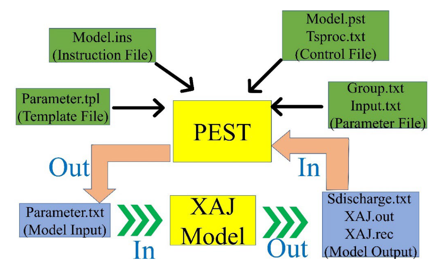
Appendix A


| Number | Name | Description |
|---|---|---|
| I | Sdischarge.txt | Simulation discharge results by initial parameter values Format: identifier (estimate/test); date (YYYYMMDD HHMMSS); simulated discharge (m3/s) |
| II | Odischarge.txt | Observed discharge (m3/s) Format: same as Sdischarge.txt |
| III | Parameter.txt | Parameter file Format: initial parameter values; parameter’s name; parameter ranges |
| IV | Parameter.tpl | Files with parameter templates Format: identifier (ptf #); # Parameter name; parameter ranges |
| V | Group.txt | Parameter group file Format: parameter’s name; type; initial values; upper bounds; lower bounds; parameter group |
| VI | Tsproc.txt | Time series control file |
| VII | Model.pst | The PEST control file provides the PEST program with the names of all the files with templates and instructions, the names of the appropriate input and output files of the model, the values of the control variables, the values of the initial parameters, the measurement value, and the weights (* parameter data) |
| VIII | Model.ins | One for each model output file from which to read numbers, and files with parameter templates (.tpl); one for each model input file with parameters from calibrating the model that manages the calibration application. (pif $) |
| IX | Tsproc.txt | Time series control file Set keywords and date formats Read Sdischarge.txt and Odischarge.txt and Write output file (Simulated discharge, model.pst and model.ins) |
| X | XAJ.rec | The results of the calculation process for each iteration |
References
- Willner, S.N.; Otto, C.; Levermann, A. Global economic response to river floods. Nat. Clim Change 2018, 8, 594–598. [Google Scholar] [CrossRef]
- Costache, R.; Bui, D.T. Spatial prediction of flood potential using new ensembles of bivariate statistics and artificial intelligence: A case study at the Putna river catchment of Romania. Sci. Total Environ. 2019, 691, 1098–1118. [Google Scholar] [CrossRef]
- Toosi, A.S.; Calbimonte, G.H.; Nouri, H.; Alaghmand, S. River basin-scale flood hazard assessment using a modified multi-criteria decision analysis approach: A case study. J. Hydrol. 2019, 574, 660–671. [Google Scholar] [CrossRef]
- Tsakiris, G. Flood risk assessment: Concepts, modelling, applications. Nat. Hazards Earth Syst. Sci. 2014, 14, 1361–1369. [Google Scholar] [CrossRef]
- Dottori, F.; Szewczyk, W.; Ciscar, J.C.; Zhao, F.; Alfieri, L.; Hirabayashi, Y.; Bianchi, A.; Mongelli, I.; Frieler, K.; Betts, R.A.; et al. Increased human and economic losses from river flooding with anthropogenic warming. Nat. Clim. Change 2018, 8, 1021. [Google Scholar] [CrossRef]
- Rehman, S.; Sahana, M.; Hong, H.Y.; Sajjad, H.; Ahmed, B.B. A systematic review on approaches and methods used for flood vulnerability assessment: Framework for future research. Nat. Hazards 2019, 96, 975–998. [Google Scholar] [CrossRef]
- Mateo-Garcia, G.; Veitch-Michaelis, J.; Smith, L.; Oprea, S.V.; Schumann, G.; Gal, Y.; Baydin, A.G.; Backes, D. Towards global flood mapping onboard low cost satellites with machine learning. Sci. Rep. 2021, 11, 7249. [Google Scholar] [CrossRef]
- Luo, P.P.; He, B.; Takara, K.; Xiong, Y.E.; Nouer, D.; Duan, W.L.; Fukushi, K. Historical assessment of Chinese and Japanese flood management policies and implications for managing future floods. Environ. Sci. Policy 2015, 48, 265–277. [Google Scholar] [CrossRef]
- Song, S.; Xu, Y.P.; Wu, Z.F.; Deng, X.J.; Wang, Q. The relative impact of urbanization and precipitation on long-term water level variations in the Yangtze River Delta. Sci. Total Environ. 2019, 648, 460–471. [Google Scholar] [CrossRef]
- Shi, J.; Cui, L.L.; Tian, Z. Spatial and temporal distribution and trend in flood and drought disasters in East China. Environ. Res. 2020, 185, 109406. [Google Scholar] [CrossRef]
- Icyimpaye, G.; Abdelbaki, C.; Mourad, K.A. Hydrological and hydraulic model for flood forecasting in Rwanda. Modeling Earth Syst. Environ. 2021, 8, 1179–1189. [Google Scholar] [CrossRef]
- Segura-Beltran, F.; Sanchis-Ibor, C.; Morales-Hernandez, M.; Gonzalez-Sanchis, M.; Bussi, G.; Ortiz, E. Using post-flood surveys and geomorphologic mapping to evaluate hydrological and hydraulic models: The flash flood of the Girona River (Spain) in 2007. J. Hydrol. 2016, 541, 310–329. [Google Scholar] [CrossRef]
- Sood, A.; Smakhtin, V. Global hydrological models: A review. Hydrol. Sci. J. 2015, 60, 549–565. [Google Scholar] [CrossRef]
- Bierkens, M.F.P. Global hydrology 2015: State, trends, and directions. Water Resour. Res. 2015, 51, 4923–4947. [Google Scholar] [CrossRef]
- Fatichi, S.; Vivoni, E.R.; Ogden, F.L.; Ivanov, V.Y.; Mirus, B.; Gochis, D.; Downer, C.W.; Camporese, M.; Davison, J.H.; Ebel, B.A.; et al. An overview of current applications, challenges, and future trends in distributed process-based models in hydrology. J. Hydrol. 2016, 537, 45–60. [Google Scholar] [CrossRef]
- Guo, Y.; Zhang, Y.; Zhang, L.; Wang, Z. Regionalization of hydrological modeling for predicting streamflow in ungauged catchments: A comprehensive review. WIREs Water 2020, 8, e1487. [Google Scholar] [CrossRef]
- Johnston, R.; Smakhtin, V. Hydrological Modeling of Large river Basins: How Much is Enough? Water Resour. Manag. 2014, 28, 2695–2730. [Google Scholar] [CrossRef]
- Zhao, R.J. The Xinanjiang Model Applied in China. J. Hydrol. 1992, 135, 371–381. [Google Scholar] [CrossRef]
- Beven, K. TOPMODEL: A critique. Hydrol. Process. 1997, 11, 1069–1085. [Google Scholar] [CrossRef]
- Liang, X.; Lettenmaier, D.P.; Wood, E.F. One-dimensional statistical dynamic representation of subgrid spatial variability of precipitation in the two-layer variable infiltration capacity model. J. Geophys Res. Atmos. 1996, 101, 21403–21422. [Google Scholar] [CrossRef]
- Zotz, G.; Thomas, V. How much water is in the tank? Model calculations for two epiphytic bromeliads. Ann. Bot. 1999, 83, 183–192. [Google Scholar] [CrossRef]
- Nascimento, N.D.; Yang, X.I.; Makhlouf, Z.; Michel, C. GR3J: A daily watershed model with three free parameters. Hydrol. Sci. J. 1999, 44, 263–277. [Google Scholar] [CrossRef]
- Yang, X.L.; Michel, C. Flood forecasting with a watershed model: A new method of parameter updating. Hydrol. Sci. J. 2000, 45, 537–546. [Google Scholar] [CrossRef]
- Lei, X.H.; Liao, W.H.; Wang, Y.H.; Jiang, Y.Z.; Wang, H.; Tian, Y. Development and Application of a Distributed Hydrological Model: EasyDHM. J. Hydrol. Eng. 2014, 19, 44–59. [Google Scholar] [CrossRef]
- Zhang, R.; Cuartas, L.A.; Carvalho, L.V.D.; Leal, K.R.D.; Mendiondo, E.M.; Abe, N.; Birkinshaw, S.; Mohor, G.S.; Seluchi, M.E.; Nobre, C.A. Season-based rainfall-runoff modelling using the probability-distributed model (PDM) for large basins in southeastern Brazil. Hydrol. Process. 2018, 32, 2217–2230. [Google Scholar] [CrossRef]
- Todini, E. The ARNO rainfall-runoff model. J. Hydrol. 1996, 175, 339–382. [Google Scholar] [CrossRef]
- Wren, S.A.C.; Rowe, R.C. Theoretical Aspects of Chiral Separation in Capillary Electrophoresis.1. Initial Evaluation of a Model. J. Chromatogr. 1992, 603, 235–241. [Google Scholar] [CrossRef]
- Arnold, J.G.; Srinivasan, R.; Muttiah, R.S.; Williams, J.R. Large area hydrologic modeling and assessment-Part 1: Model development. J. Am. Water Resour. Assoc. 1998, 34, 73–89. [Google Scholar] [CrossRef]
- Xu, C.; Wang, Y.; Fu, H.; Yang, J. Comprehensive Analysis for Long-Term Hydrological Simulation by Deep Learning Techniques and Remote Sensing. Front. Earth Sci. 2022, 10, 875145. [Google Scholar] [CrossRef]
- Geris, J.; Tetzlaff, D.; Seibert, J.; Vis, M.; Soulsby, C. Conceptual Modelling to Assess Hydrological Impacts and Evaluate Environmental Flow Scenarios in Montane River Systems Regulated for Hydropower. River Res. Appl. 2015, 31, 1066–1081. [Google Scholar] [CrossRef]
- Crawford, N.H.; Linsley, R.K. Digital Simulation in Hydrology: Stanford Watershed Model IV; Evapotranspiration; Department of Civil Engineering Stanford University: Stanford, CA, USA, 1966. [Google Scholar]
- Moore, R.J. The PDM rainfall-runoff model. Hydrol. Earth Syst. Sci. 2007, 11, 483–499. [Google Scholar] [CrossRef]
- Jiang, T.; Chen, Y.Q.D.; Xu, C.Y.Y.; Chen, X.H.; Chen, X.; Singh, V.P. Comparison of hydrological impacts of climate change simulated by six hydrological models in the Dongjiang Basin, South China. J. Hydrol. 2007, 336, 316–333. [Google Scholar] [CrossRef]
- Zhang, Y.Q.; Chiew, F.H.S. Relative merits of different methods for runoff predictions in ungauged catchments. Water Resour. Res. 2009, 45, W07412. [Google Scholar] [CrossRef]
- Gong, J.F.; Yao, C.; Li, Z.J.; Chen, Y.F.; Huang, Y.C.; Tong, B.X. Improving the flood forecasting capability of the Xinanjiang model for small- and medium-sized ungauged catchments in South China. Nat. Hazards 2021, 106, 2077–2109. [Google Scholar] [CrossRef]
- Bai, P.; Liu, X.M.; Liang, K.; Liu, X.J.; Liu, C.M. A comparison of simple and complex versions of the Xinanjiang hydrological model in predicting runoff in ungauged basins. Hydrol. Res. 2017, 48, 1282–1295. [Google Scholar] [CrossRef]
- Zhao, L.L.; Xia, J.; Xu, C.Y.; Wang, Z.G.; Sobkowiak, L.; Long, C.R. Evapotranspiration estimation methods in hydrological models. J. Geogr. Sci. 2013, 23, 359–369. [Google Scholar] [CrossRef]
- Song, X.M.; Zhang, J.Y.; Zhan, C.S.; Xuan, Y.Q.; Ye, M.; Xu, C.G. Global sensitivity analysis in hydrological modeling: Review of concepts, methods, theoretical framework, and applications. J. Hydrol. 2015, 523, 739–757. [Google Scholar] [CrossRef]
- Dong, C.Y. Remote sensing, hydrological modeling and in situ observations in snow cover research: A review. J. Hydrol. 2018, 561, 573–583. [Google Scholar] [CrossRef]
- Praskievicz, S.; Chang, H.J. A review of hydrological modelling of basin-scale climate change and urban development impacts. Prog. Phys. Geogr. 2009, 33, 650–671. [Google Scholar] [CrossRef]
- Gao, H.K.; Sabo, J.L.; Chen, X.H.; Liu, Z.Y.; Yang, Z.J.; Ren, Z.; Liu, M. Landscape heterogeneity and hydrological processes: A review of landscape-based hydrological models. Landsc. Ecol. 2018, 33, 1461–1480. [Google Scholar] [CrossRef]
- Dong, Q.Q.; Zhan, C.S.; Wang, H.X.; Wang, F.Y.; Zhu, M.C. A review on evapotranspiration data assimilation based on hydrological models. J. Geogr. Sci. 2016, 26, 230–242. [Google Scholar] [CrossRef][Green Version]
- Fernández-Pato, J.; Caviedes-Voullième, D.; García-Navarro, P. Rainfall/runoff simulation with 2D full shallow water equations: Sensitivity analysis and calibration of infiltration parameters. J. Hydrol. 2016, 536, 496–513. [Google Scholar] [CrossRef]
- Costabile, P.; Costanzo, C. A 2D-SWEs framework for efficient catchment-scale simulations: Hydrodynamic scaling properties of river networks and implications for non-uniform grids generation. J. Hydrol. 2021, 599, 126306. [Google Scholar] [CrossRef]
- Hien, L.T.T.; Chien, N.V. Investigate Impact Force of Dam-Break Flow against Structures by Both 2D and 3D Numerical Simulations. Water 2021, 13, 344. [Google Scholar] [CrossRef]
- Wang, G.T.; Chen, S.; Boll, J. A semianalytical solution of the Saint-Venant equations for channel flood routing. Water Resour. Res. 2003, 39, 1076. [Google Scholar] [CrossRef]
- Zarmehi, F.; Tavakoli, A. A Simple Scheme to Solve Saint-Venant Equations by Finite Element Method. Int. J. Comput. Methods 2016, 13, 1650001. [Google Scholar] [CrossRef]
- Yu, C.W.; Hodges, B.; Liu, F. A new form of the Saint-Venant equations for variable topography. Hydrol. Earth Syst. Sci. 2020, 24, 4001–4024. [Google Scholar] [CrossRef]
- Yang, X.; An, W.; Li, W.; Zhang, S. Implementation of a Local Time Stepping Algorithm and Its Acceleration Effect on Two-Dimensional Hydrodynamic Models. Water 2020, 12, 1148. [Google Scholar] [CrossRef]
- Kim, B.; Sanders, B.F.; Schubert, J.E.; Famiglietti, J.S. Mesh type tradeoffs in 2D hydrodynamic modeling of flooding with a Godunov-based flow solver. Adv. Water Resour. 2014, 68, 42–61. [Google Scholar] [CrossRef]
- Xia, X.L.; Liang, Q.H.; Ming, X.D. A full-scale fluvial flood modelling framework based on a high-performance integrated hydrodynamic modelling system (HiPIMS). Adv. Water Resour. 2019, 132, 103392. [Google Scholar] [CrossRef]
- Liang, Q.H.; Smith, L.S. A high-performance integrated hydrodynamic modelling system for urban flood simulations. J. Hydroinform. 2015, 17, 518–533. [Google Scholar] [CrossRef]
- Fernandez, A.; Najafi, M.R.; Durand, M.; Mark, B.G.; Moritz, M.; Jung, H.C.; Neal, J.; Shastry, A.; Laborde, S.; Phang, S.C.; et al. Testing the skill of numerical hydraulic modeling to simulate spatiotemporal flooding patterns in the Logone floodplain, Cameroon. J. Hydrol. 2016, 539, 265–280. [Google Scholar] [CrossRef]
- Xu, C.W.; Han, Z.Y.; Fu, H. Remote Sensing and Hydrologic-Hydrodynamic Modeling Integrated Approach for Rainfall-Runoff Simulation in Farm Dam Dominated Basin. Front. Environ. Sci. 2022, 9, 672. [Google Scholar] [CrossRef]
- Sauvagnargues, S.; Salze, D.; AyralP, A.; Laganier, O. A coupling of hydrologic and hydraulic models appropriate for the fast floods of the Gardon River basin (France). Nat. Hazards Earth Syst. Sci. 2014, 14, 2899–2920. [Google Scholar]
- Sherman, L. Streamflow from rainfall by the unit-graph method. Eng. News Rec. 1932, 108, 501–505. [Google Scholar]
- Luo, B. Theory and application of lag-and-route method and comparison with other flood routing methods. J. Hydraul. Eng. 1987, 32, 485–496. (In Chinese) [Google Scholar]
- Monajemi, P.; Khaleghi, S.; Maleki, S. Derivation of instantaneous unit hydrographs using linear reservoir models. Hydrol. Res. 2021, 52, 339–355. [Google Scholar] [CrossRef]
- Gill, M.A. Flood Routing by the Muskingum Method-Reply. J. Hydrol. 1979, 41, 169–170. [Google Scholar] [CrossRef]
- Liang, Q.H.; Smith, L.; Xia, X.L. New prospects for computational hydraulics by leveraging high-performance heterogeneous computing techniques. J. Hydrodyn. 2016, 28, 977–985. [Google Scholar] [CrossRef]
- Wang, W.Q.; Chen, W.J.; Huang, G.R. Urban Stormwater Modeling with Local Inertial Approximation Form of Shallow Water Equations: A Comparative Study. Int. J. Disaster Risk Sci. 2021, 12, 745–763. [Google Scholar] [CrossRef]
- Chao, L.J.; Zhang, K.; Li, Z.J.; Wang, J.F.; Yao, C.; Li, Q.L. Applicability assessment of the CASCade Two Dimensional SEDiment (CASC2D-SED) distributed hydrological model for flood forecasting across four typical medium and small watersheds in China. J. Flood Risk Manag. 2019, 12, e12518. [Google Scholar] [CrossRef]
- Wagner, P.D.; Fiener, P.; Wilken, F.; Kumar, S.; Schneider, K. Comparison and evaluation of spatial interpolation schemes for daily rainfall in data scarce regions. J. Hydrol. 2012, 464, 388–400. [Google Scholar] [CrossRef]
- Goegebeur, M.; Pauwels, V.R.N. Improvement of the PEST parameter estimation algorithm through Extended Kalman Filtering. J. Hydrol. 2007, 337, 436–451. [Google Scholar] [CrossRef]
- Li, X.H.; Zhang, Q.; Shao, M.; Li, Y.L. A comparison of parameter estimation for distributed hydrological modelling using automatic and manual methods. Adv. Mater. Res. 2012, 356–360, 2372–2375. [Google Scholar] [CrossRef]
- Li, H.X.; Zhang, Y.Q.; Chiew, F.H.S.; Xu, S.G. Predicting runoff in ungauged catchments by using Xinanjiang model with MODIS leaf area index. J. Hydrol. 2009, 370, 155–162. [Google Scholar] [CrossRef]
- Yao, C.; Zhang, K.; Yu, Z.B.; Li, Z.J.; Li, Q.L. Improving the flood prediction capability of the Xinanjiang model in ungauged nested catchments by coupling it with the geomorphologic instantaneous unit hydrograph. J. Hydrol. 2014, 517, 1035–1048. [Google Scholar] [CrossRef]
- Lin, K.R.; Lv, F.S.; Chen, L.; Singh, V.P.; Zhang, Q.; Chen, X.H. Xinanjiang model combined with Curve Number to simulate the effect of land use change on environmental flow. J. Hydrol. 2014, 519, 3142–3152. [Google Scholar] [CrossRef]
- Li, Z.J.; Kan, G.Y.; Yao, C.; Liu, Z.Y.; Li, Q.L.; Yu, S. Improved Neural Network Model and Its Application in Hydrological Simulation. J. Hydrol. Eng. 2014, 19, 04014019. [Google Scholar] [CrossRef]
- Wang, Y.L.; Yang, X.L. A Coupled Hydrologic-Hydraulic Model (XAJ-HiPIMS) for Flood Simulation. Water 2020, 12, 1288. [Google Scholar] [CrossRef]
- Moriasi, D.N.; Gitau, M.W.; Pai, N.; Daggupati, P. Hydrologic and Water Quality Models: Performance Measures and Evaluation Criteria. Trans. ASABE 2015, 58, 1763–1785. [Google Scholar]
- Amo-Boateng, M.; Li, Z.J.; Guan, Y.Q. Inter-annual variation of streamflow, precipitation and evaporation in a small humid watershed (Chengcun Basin, China). Chin. J. Oceanol. Limnol. 2014, 32, 455–468. [Google Scholar] [CrossRef]


| Hydrological Model | Developed/Maintained by | Type | Runoff Characteristic | Applications |
|---|---|---|---|---|
| XAJ | Zhao, 1984 | Lumped | Saturation—excess runoff | Humid/semihumid Hourly/daily |
| TOPMODEL | Beven and Kirkby, 1979 | Semidistributed | Saturation—excess runoff | Humid/arid Daily |
| VIC | Liang et al., 1994 | Distributed | Infiltration—excess runoff | Daily/monthly River basin |
| TANK | Sugawara, 1961 | Lumped | Infiltration—excess runoff | Single rainfall simulation Humid/arid |
| GR3 | Edijaton, 1999 | Lumped | Saturation—excess runoff | Hourly/daily Small/medium watershed |
| GR4 J | Perrin et al., 1993 | Lumped | Saturation—excess runoff | Hourly/daily Small/middle watershed |
| EasyDHM | Lei, X., et al., 2010 | Distributed | Saturation—excess/infiltration—excess | Wide applicability |
| PDM | University of Reading, UK, 1998 | Lumped | Saturation—excess runoff | Daily Continuous simulation A macroscale globe model |
| ARNO | Ciarapica, Todini, 1996, 2002 | Lumped/ distributed | Saturation-excess runoff | Large range of spatial scales Continuous simulation |
| SAC | Burnash, Ferral, Ferral, 1970s | Lumped | Saturation—excess runoff | Long-time continuous simulation Daily/6 h Large/medium watershed Humid/arid |
| SWAT | Arnold et al., 1995 | Distributed | Infiltration—excess runoff | Up to large river basin Daily/monthly |
| HBV | Gardelin, 1997 | Lumped/ Distributed | Saturation—excess runoff | Large/medium watershed Daily/donthly |
| SWM | Linsley, Crawford,1959 | Lumped | Saturation—excess runoff | Continuous simulation Hourly |
| Parameter | Physical Meaning | Range and Units [66,67,68] | Value | |
|---|---|---|---|---|
| (Hourly Model) [69] | ||||
| Evapotranspiration | K | Evaporation coefficient | 0.5–1.1 (-) | 0.8 |
| C | Evaporation coefficient of the deep layer | 0.1–0.3 (-) | 0.1 | |
| WUM | Tension water capacity of upper layer | 5–100 (mm) | 17 | |
| WLM | Tension water capacity of lower layer | 50–300 (mm) | 87 | |
| WDM | Tension water capacity of deep layer | 5–100 (mm) | 33 | |
| Runoff generation | B | Representation of the nonuniformity of the spatial distribution of the tension water capacity | 0.1–2 (-) | 0.3 |
| IMP | Proportion of impervious surface | 0.01–0.1 (%) | 0.01 | |
| Runoff separation | SM | Mean free water storage capacity | 5–100 (mm) | 97 |
| EX | The distribution of free water storage capacity | 1–1.5 (-) | 1.5 | |
| Runoff routing | KSS | Outflow coefficient of the free water storage reservoir to interflow | 0.01–0.7 (-) | 0.4 |
| KG | Outflow coefficient of the free water storage reservoir to groundwater | 0.01–0.7 (-) | 0.3 | |
| KKI | Recession coefficient of the interflow | 0.05–0.95 (-) | 0.9 | |
| KKG | Recession coefficient of the groundwater | 0.9–0.999 (-) | 0.98 |
| Land Use | Manning’s Coefficient (s/[m1/3]) |
|---|---|
| Urban land | 0.013 |
| Water | 0.021 |
| Grassland | 0.031 |
| Cultivated land | 0.041 |
| Forest land | 0.139 |
| Land Use | 1990 | 1991 | 1992 | 1993 | 1994 | 1995 | 1996 | |||||||
|---|---|---|---|---|---|---|---|---|---|---|---|---|---|---|
| Area | Ratio(%) | Area | Ratio(%) | Area | Ratio(%) | Area | Ratio(%) | Area | Ratio(%) | Area | Ratio(%) | Area | Ratio(%) | |
| Cultivated land | 1.44 | 0.51 | 1.62 | 0.58 | 1.70 | 0.61 | 1.80 | 0.64 | 1.80 | 0.64 | 1.75 | 0.62 | 1.68 | 0.60 |
| Forest | 279.33 | 99.43 | 279.14 | 99.36 | 279.06 | 99.33 | 278.95 | 99.30 | 278.96 | 99.30 | 279.02 | 99.32 | 279.09 | 99.35 |
| Grass land | 0.11 | 0.04 | 0.11 | 0.04 | 0.09 | 0.03 | 0.09 | 0.03 | 0.09 | 0.03 | 0.08 | 0.03 | 0.08 | 0.03 |
| Water | 0.01 | 0.00 | 0.02 | 0.01 | 0.03 | 0.01 | 0.02 | 0.01 | 0.01 | 0.00 | 0.02 | 0.01 | 0.01 | 0.00 |
| Urban land | 0.04 | 0.01 | 0.05 | 0.02 | 0.06 | 0.02 | 0.07 | 0.02 | 0.07 | 0.02 | 0.07 | 0.02 | 0.07 | 0.02 |
| Flood Code | Rainfall (mm) | RE (%) | PE (%) | NSE | |||||
|---|---|---|---|---|---|---|---|---|---|
| XAJ | 2D | XAJ | 2D | XAJ | 2D | XAJ | 2D | ||
| 19900614 | 112.88 | 31.61 | 36.13 | 10.58 | 13.54 | 0.85 | 0.77 | 0 | 0 |
| 19900626 | 246.09 | 18.23 | 4.68 | 18.86 | 6.02 | 0.90 | 0.85 | 7 | 3 |
| 19910518 | 158.97 | 8.24 | 26.17 | 13.80 | 7.21 | 0.86 | 0.64 | 1 | 3 |
| 19920516 | 81.58 | 19.45 | 19.75 | 25.45 | 17.27 | 0.83 | 0.56 | 0 | 3 |
| 19920701 | 225.62 | 31.45 | 1.16 | 6.25 | 15.03 | 0.87 | 0.57 | 0 | 6 |
| 19930629 | 566.69 | 17.16 | 2.51 | 14.62 | 11.61 | 0.90 | 0.83 | 1 | 4 |
| 19940608 | 574.15 | 14.96 | 10.38 | 5.14 | 19.53 | 0.83 | 0.80 | 2 | 7 |
| 19950519 | 500.78 | 17.10 | 9.02 | 24.17 | 12.56 | 0.69 | 0.64 | 1 | 3 |
| 19950701 | 160.98 | 26.76 | 6.41 | 18.70 | 11.13 | 0.79 | 0.80 | 1 | 3 |
| 19960619 | 169.21 | 2.99 | 19.12 | 20.84 | 1.81 | 0.62 | 0.91 | 0 | 4 |
Publisher’s Note: MDPI stays neutral with regard to jurisdictional claims in published maps and institutional affiliations. |
© 2022 by the authors. Licensee MDPI, Basel, Switzerland. This article is an open access article distributed under the terms and conditions of the Creative Commons Attribution (CC BY) license (https://creativecommons.org/licenses/by/4.0/).
Share and Cite
Xu, C.; Yang, J.; Wang, L. Application of Remote-Sensing-Based Hydraulic Model and Hydrological Model in Flood Simulation. Sustainability 2022, 14, 8576. https://doi.org/10.3390/su14148576
Xu C, Yang J, Wang L. Application of Remote-Sensing-Based Hydraulic Model and Hydrological Model in Flood Simulation. Sustainability. 2022; 14(14):8576. https://doi.org/10.3390/su14148576
Chicago/Turabian StyleXu, Chaowei, Jiashuai Yang, and Lingyue Wang. 2022. "Application of Remote-Sensing-Based Hydraulic Model and Hydrological Model in Flood Simulation" Sustainability 14, no. 14: 8576. https://doi.org/10.3390/su14148576
APA StyleXu, C., Yang, J., & Wang, L. (2022). Application of Remote-Sensing-Based Hydraulic Model and Hydrological Model in Flood Simulation. Sustainability, 14(14), 8576. https://doi.org/10.3390/su14148576