Regional Differences and Spatial Convergence of Green Development in China

Abstract

Green development is an important path to achieving economic, environmental, and social sustainability. Based on the comprehensive evaluation system of economy, environment, and society, this study used the entropy method, Theil index decomposition method, and spatial β-convergence model to study the differences and spatial convergence of China’s green development from 2010 to 2020. The research conclusions are as follows: First, China’s green development has an upward trend, and the eastern region is higher. Second, the regional differences in green development have the characteristic of rising first and then falling, and the differences within regions are the main source of imbalances in China’s green development. Third, China’s green development has obvious characteristics of spatial absolute β-convergence and spatial conditional β-convergence. Green innovation is conducive to narrowing the gaps in the convergence speed of regional green development. The research results comprehensively explain the characteristics of China’s green development and provide realistic evidence for China’s green development in the future.

1. Introduction

Sustainability has been a research focus since the 1980s. In 1987, the World Commission on Environment and Development (WCED) proposed that sustainability is a development model that can meet the needs of the present without compromising the interests of future generations. It reflects the coordination of the economy, resources, environment, and society [1]. To achieve the goal of sustainable development, people have actively explored and formed a green development path centered on ‘green transformation’ [2,3]. Green development (GD) is a new model that integrates economic growth, environmental protection, and social development. It aims to increase economic efficiency, promote social equity, and improve the ecological environment [3,4]. The Chinese government has been committed to green transformation and development. In 2003, the Chinese government formulated a coordinated development strategy for sustainable economic, environmental, and social development [5]. In 2010, it was proposed to rely on green transformation to promote sustainable development and strive to achieve GD by 2050. This study focused on the reality of China’s GD and studied three issues: first, how to scientifically calculate the level of GD in China’s regions; second, how to identify the regional differences in China’s GD; third, how to identify the evolutionary characteristics of regional GD.

In the process of urbanization and industrialization, scholars have proposed different theoretical systems of GD. In economic terms, the green economy and green finance are the embodiment of the economic efficiency of GD [6,7]. The green economy is a new market-economy model focusing on resource conservation and ecological protection, aimed at the coordinated development of the economy and the environment [8]. The green economy can promote economic sustainability by improving energy efficiency, changing production methods, optimizing industrial structure, increasing foreign investment, and optimizing capital allocation [9,10,11,12]. The data envelopment analysis (DEA) and slack-based models (SBM) are effective methods of measuring the efficiency of the green economy [13,14]. In terms of the environment, carbon neutrality, carbon trading, pollution control, and environmental regulation reflect the environmental efficiency of GD [15,16]. The government restricts the pollutant emissions of enterprises by implementing environmental regulations [17]. Carbon trading markets can control total carbon dioxide emissions [18]. In addition, the government’s investment in environmental governance and enterprises’ commitment to environmental responsibility have promoted regional GD [19]. In terms of technology, clean energy technology, green material technology, resource-recycling technology, and pollutant-treatment technology reflect the technological effect of green innovation [20,21,22,23]. Technological innovation is essential for promoting the green transformation of enterprises. On one hand, technological innovation reduces traditional resource consumption and pollution emissions by adjusting the combination of production factors [24]. On the other hand, the technological development of renewable energy reduces the production cost of enterprises and increases the industrial-added value [25]. In terms of a comprehensive evaluation, sustainable development consists of the three subsystems of economy, environment, and society; the coupling and coordination between them can scientifically reflect the efficiency of GD [26]. In addition, inclusiveness is also a focus of green development. Residents’ life, health care, income equality, and education are factors that affect regional GD [27,28,29,30]. Social network analysis (SNA), analytic hierarchy process (AHP), entropy method, and principal component analysis (PCA) are the main methods of examining the relationship between the economy, environment, and society [26,31].

Studies of different dimensions explain GD’s economic–environmental relationship, but there are still research gaps. First, technological innovation is the path to improving the green economy and environmental quality. In addition to the economic and environmental effects, GD also includes social effects. The existing studies ignore the fact that social effects cannot scientifically reflect the realistic characteristics of GD. Therefore, within the three-dimensional framework of the economy, environment, and society, the scientific measurement of the GD is a problem that needs to be studied. In addition, the regional differences and development trends of green development also need attention. Due to the limitations of population, resource endowment, economic foundation, education, industrial foundation, and other conditions, the ability of GD in developed and developing regions is different, which also leads to regional gaps [32]. Although the spatial correlation between the economic and environmental effects of GD has been confirmed [33], there is a lack of research on the regional differences and spatial trends of GD. GD is a process of dynamic change. It pays attention only to the static spatial characteristics of the green economy and environmental governance and ignores the dynamic evolution trend of GD, which cannot scientifically reflect the characteristics of GD.

The research contributions of this study are as follows. First, this study constructed a three-dimensional GD evaluation system of the economy, environment, and society, which is different from researchers who only focus on the relationship between the economy and environment, but it considered the social effect of GD. A multi-dimensional evaluation system can improve the measurement accuracy of GD. Second, the Theil index was used to decompose the differences of GD in various regions of China. The within-group differences, between-group differences, and their contribution rates of GD were investigated. This helped to clarify the source of the regional differences of the GD and provided new evidence for the different regions to formulate differentiated green-transition strategies. Third, the spatial β-convergence model was used to test the convergence of the regional GD, showing the characteristics of the spatial evolution of China’s regional GD, which can make up for the fact that scholars have more static research on GD and insufficient dynamic analysis.

2. Materials

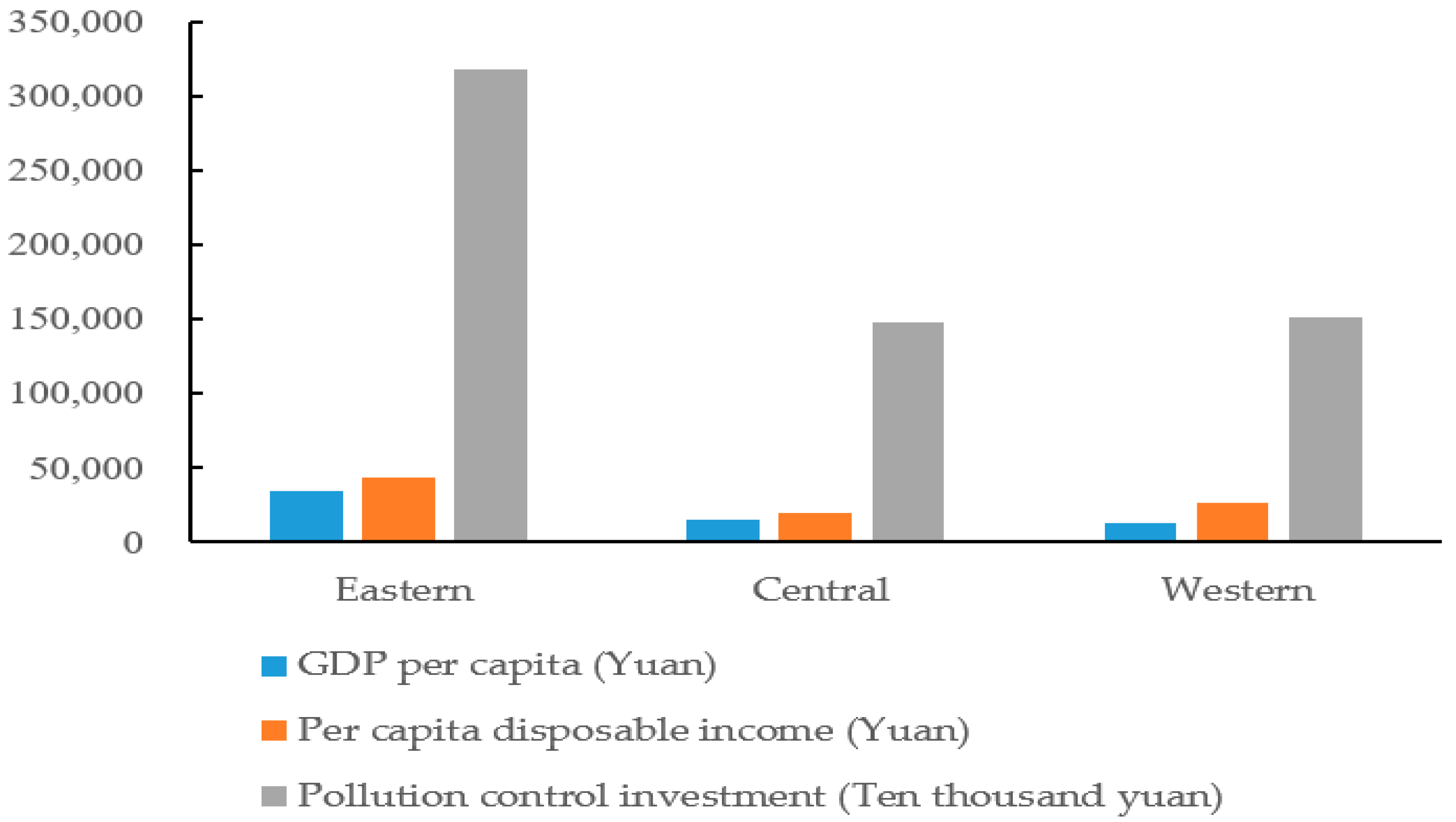
2.1. Research Scenario

Over the past 40 years, China’s economic achievements have been evident. Under the traditional economic growth model, extensive resource development has accumulated a lot of wealth for China. Still, it has also exacerbated the contradiction between resources, the environment, and residents’ lives, and it has resulted in unbalanced regional development [32]. The eastern cities took the lead in realizing development through policy support, and their economic foundation, industrial structure, technical level, energy structure, and living habits all have obvious advantages. The economic conditions of the central and western cities lag, the per capita income is low, and they have received a large number of heavy industry transfers from the eastern cities. As shown in Figure 1, between 2011 and 2020, the economic conditions (GDP per capita), environmental protection investment (pollution control), and residents’ living (per capita disposable income) in the eastern region were higher. These gaps led to differences in the ability of GD in different regions. Therefore, the research on China’s GD should not only make a comprehensive assessment of the total amount but also clarify the regional characteristics. In addition, the analysis of the convergence can clarify the dynamic evolution trend of GD in China, which helps to improve the coordination of GD between regions and then accelerate the process of GD across the country. This study took 30 provinces in China from 2011 to 2020 as a research sample, built an economic–environment–social evaluation system to measure China’s GD, clarified the regional differences, and analyzed the evolution trend. These can provide evidence for China’s goal of achieving comprehensive green development by 2050.

2.2. Research Data

Considering the completeness of the data, the sample data selected in this study were a panel data of 30 provinces in mainland China from 2011 to 2020 (excluding Tibet with missing data). Since the data of GD involve regional economic development, the ecological environment, and the reality of residents’ lives, the research data in this study were also obtained through the government’s public reports. The regional economic data mainly come from the National Bureau of Statistics of China, the regional environmental data come from the China Energy Statistical Yearbook and the China Environmental Statistical Yearbook, and the regional social life data come from the China Regional Economic Development Yearbook.

3. Methods

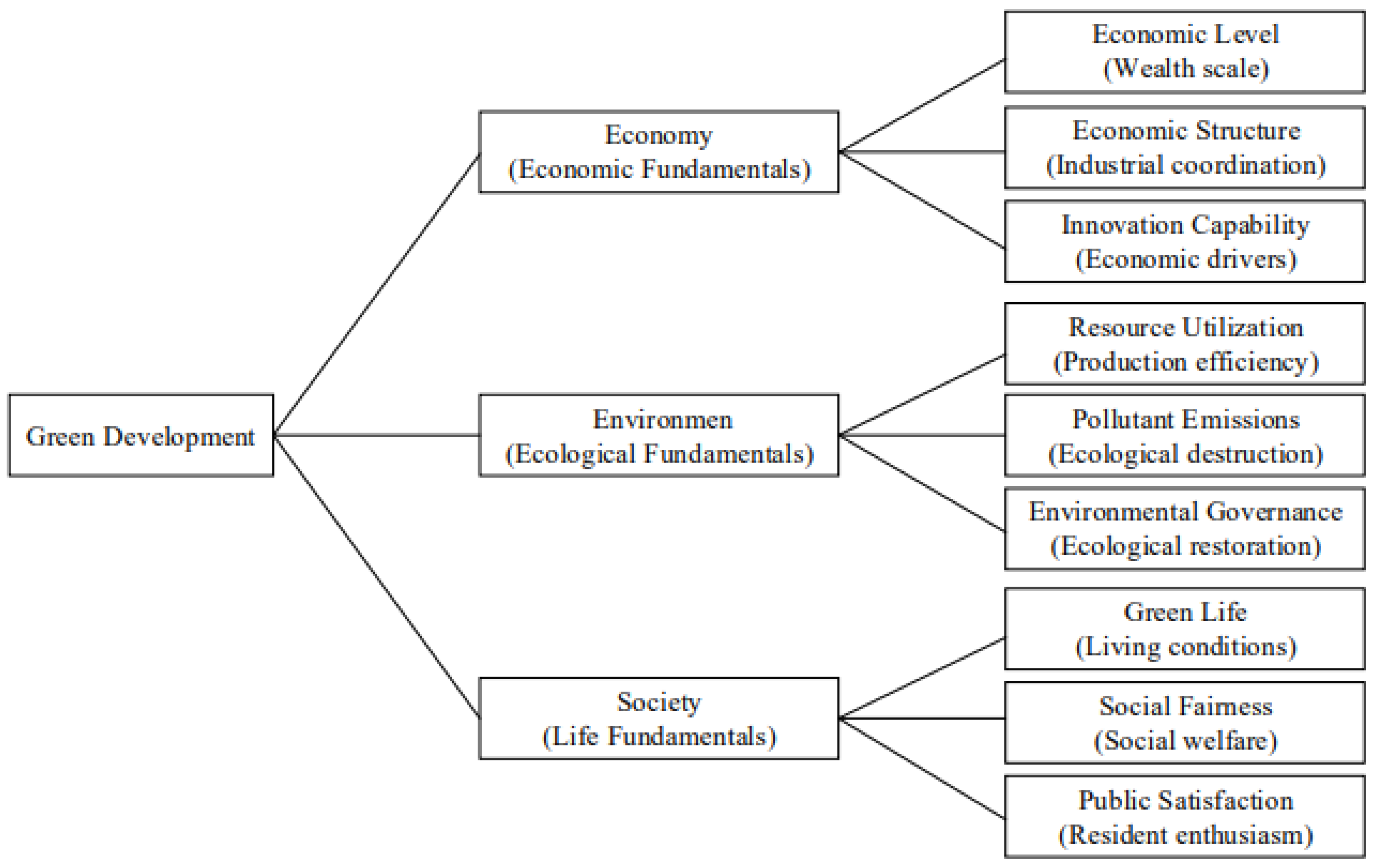
3.1. Indicator System and Calculation Method of GD

3.1.1. Indicator System

GD is the coordinated development of the economy, environment, and society. The improvement of resource utilization efficiency and the application of green technology are the intermediate paths to drive green development. They play a role in regional economic growth, environmental governance, and social life by affecting enterprise production, residents’ consumption, pollution emissions, and energy utilization. An evaluation of green development should be results-oriented and carry out a multi-dimensional analysis. Referring to the sustainable indicator system of the United Nations’ Commission on Sustainable Development (UNCSD) and the “Green Development Indicator System” of the National Development and Reform Commission of China [34], this study mainly constructed a comprehensive evaluation system for GD from three dimensions: the economy, environment, and society, as shown in Figure 2. The economic dimension selected indicators from three aspects: the economic level, economic structure, and innovation ability, which mainly express the economic efficiency of green development. Among them, the economic level reflects the scale of social wealth, and its indicators include GDP, income, investment, and so on. The economic structure reflects the coordination degree of industrial development. Compared with the primary industry, the added value of the secondary and tertiary industries was more in line with the goal of economic sustainability. Technological innovation drives economic growth, and its indicators include R&D investment and patents. The environmental dimension selects indicators from the aspects of resource utilization, pollution discharge, and environmental governance, which mainly express the environmental efficiency of green development. Among them, resource utilization reflects energy consumption, energy structure, and production efficiency. Its indicators include per capita resource consumption, clean energy proportion, and economic value added per unit of energy. Pollutant emissions cause ecological damage, and its indicators include wastewater, waste gas, and solid waste. Environmental governance reflects ecological improvement, and its indicators include investment in pollution control and disposal of pollutants. The social dimension selects indicators from social equity, green life, and residents’ satisfaction, which mainly express the social impact of GD. Among them, green life reflects the living conditions, living environment, and lifestyle of residents. Excessive population-gathering will aggravate the destruction of the urban environment. Its indicators include population density, green products, green buildings, green transportation, and green area. Social fairness reflects public welfare; equal social status is conducive to the green transformation of the city, and its indicators include income, education, and medical care. Public satisfaction reflects the residents’ expectations and enthusiasm for improving their living environment. The index system is shown in

Table 1. Evaluation system of GD.

System	Description	Indicator	Correlation	Reference
Economic system	Economic level	Gross domestic product (yuan)	+	[35,36,37]
		Per capita disposable income (yuan)	+
		Total investment in fixed assets (yuan)	+
		Foreign direct investment	+
	Economic structure	Proportion of primary industry (%)	−	[12,38]
		Proportion of secondary industry (%)	+
		Proportion of tertiary industry (%)	+
	Innovation capability	R&D expenditure (yuan)	+	[39]
		R&D personnel	+
		Number of patent applications	+
Environmental system	Resource utilization	Per capita resource consumption (standard coal)	−	[26,40]
		Proportion of clean energy (%)	+
		Ratio of GDP to total energy consumption (%)	−
		Per capita arable land (kilometers)	+
		Per capita forest area (kilometers)	+
	Pollutant emissions	Industrial wastewater discharge (ton)	−	[41,42]
		Industrial exhaust emissions (ton)	−
		Solid waste discharge (ton)	−
	Environmental governance	Government’s investment in environmental governance (yuan)	+	[43,44]
		Urban sewage treatment rate (%)	+
		Domestic waste disposal rate (%)	+
Social system	Green life	Population density (%)	−	[45,46,47]
		Proportion of green products (%)	+
		Proportion of green buildings (%)	+
		Proportion of new energy vehicles (%)	+
		Green area per capita (kilometers)	+
	Social fairness	Urban–rural income gap (%)	−	[28,29,30]
		Average education level (year)	+
		Number of beds per 10,000 people in medical institutions	+
	Public satisfaction	Residents’ satisfaction with the quality of living environment (%)	+	[48,49]

.

3.1.2. Evaluation Method

Since this study built a multi-dimensional index evaluation system for GD, it is appropriate to use the comprehensive evaluation method to measure green development. Comprehensive evaluation is a method of using multiple indicators to evaluate multiple participating units. The principal component analysis (PAC), analytic hierarchy process (AHP), and entropy method are the main methods of comprehensive evaluation. The PAC is based on the principle of the information concentration of data, and the weight is calculated by the variance explanation rate. However, the information compression intelligence obtains the weight of the comprehensive index, and the weight of the specific index cannot be obtained. The AHP calculates the weight by the relative size information of the numbers, and its subjectivity is too strong. The entropy method uses the entropy information of data to calculate the weight, which can avoid errors caused by subjectivity and can also calculate the information of specific indicators. Therefore, the entropy method was suitable for this study. The specific steps are as follows.

First, we set specific indicators and constructed a comprehensive index system including n provinces, t years, and m indicators. $X_{ij}$ is the j index in the i region.

Second, we standardized the value of the indicator. For the indicators of each evaluation object, the extreme value method was used for normalization. The normalization processing method of positive indicators is shown in Equation (1), and the negative indicators are shown in Equation (2). $X_{ij}$ is the normalized value.

$$X_{ij}=\frac{x_{ij}-\min \left(x_{ij}\right)}{\max \left(x_{ij}\right)-\min \left(x_{ij}\right)}$$

(1)

$$X_{ij}=\frac{\max \left(x_{ij}\right)-x_{kij}}{\max \left(x_{ij}\right)-\min \left(x_{ij}\right)}$$

(2)

Third, we calculated the information entropy of each index. Equation (3) was used to calculate the contribution degree ($P_{ij}$) of $X_{ij}$ in t period, and the entropy value ($E_j$) of the j index was then calculated using Equation (4). The information entropy ($d_j$) of the j index is shown in Equation (5).

$$P_{ij}=\frac{X_{ij}}{{\displaystyle \sum _{i=1}^n{X}_{ij}}}$$

(3)

$$E_j=-\frac{1}{\ln n}{\displaystyle \sum _{i=1}^n{P}_{ij}\ln }{P}_{ij}$$

(4)

$$d_j=1-E_j$$

(5)

Fourth, we calculated the weight. Combined with the results of Equation (5), the weight ($w_j$) of each index was calculated using Equation (6).

$$w_j=\frac{d_j}{{\displaystyle \sum _{j=1}^m{d}_j}}$$

(6)

Fifth, we calculated the comprehensive index of the evaluation object. Combined with the results of Equation (6), Equation (7) was used to calculate the score (S) of each indicator.

$$S={\displaystyle \sum _{j=1}^m{w}_j}{X}_{ij}$$

(7)

3.2. Calculation Method of Regional Difference

To analyze the differences of regional green development, this study adopted the Theil index decomposition method for research, including the overall gap, gap within regions, and gap between regions. The Theil index is a key method of economic inequality that can decompose the overall differences between regions into intra-group differences and inter-group differences, and more directly it can show their development trends and contribution rates to the overall differences [50]. The value range of the Theil index is [0, 1]. The larger the Theil index ($T$) is, the larger the overall gap in the region is. The calculation formula is shown in Equation (8). In Equation (8), $\overline{gd}$ is the average value of annual GD, and gd_i is the value of GD.

$$T=\frac{1}{n}{\displaystyle \sum _{i=1}^n\left(\frac{g{d}_i}{\overline{gd}}\times \ln \frac{g{d}_i}{\overline{gd}}\right)}$$

(8)

To clarify the regional differences of GD, this study decomposed the regional differences of GD into the differences within regions ($T_w$) and the differences between regions ($T_b$), as shown in Formula (9). According to the characteristics of China’s regional geography, we divided the 30 provinces into three groups: eastern, central, and western, where (k = 1, 2, 3). Among them, the eastern region comprised 11 provinces, including Beijing, Shanghai, Tianjin, Shandong, etc. The central region comprised 8 provinces, including Henan, Anhui, Hubei, Hunan, etc. The western region comprised 11 provinces, including Inner Mongolia, Chongqing, Sichuan, Yunnan, Guizhou, etc. $n_k$ is the number of samples in the kth group, and the internal difference ($T_k$) of the kth group was calculated using Equation (10). The $T_w$ was calculated using Equation (11), and the $T_b$ was calculated using Equation (12). The differences within regions contribution ($C_w$) and the differences between regions ($C_b$) of the kth group were calculated using Equation (13).

$$T=T_w+T_b$$

(9)

$$T_k={\displaystyle \sum _{i\in g{d}_k}\frac{g{d}_i}{g{d}_k}\ln \frac{g{d}_i/g{d}_k}{1/n_k}}$$

(10)

$$T_w={\displaystyle \sum _{k=1}^{K}g{d}_k({\displaystyle \sum _{i\in g{d}_k}\frac{g{d}_i}{g{d}_k}\ln \frac{g{d}_i/g{d}_k}{1/n_k}})}$$

(11)

$$T_b={\displaystyle \sum _{k=1}^{K}g{d}_k\ln \frac{g{d}_k}{n_k/n}}$$

(12)

$$C_w=g{d}_k\frac{T_k}{T}\hspace{1em}{C}_b=\frac{T_b}{T}$$

(13)

3.3. Spatial Convergence Model

In order to clarify the spatial characteristics of regional GD, this study used the β-convergence model to test the evolution trend. The β-convergence showed that lagging regions will gradually catch up with developed regions due to their faster growth rate and will reach a steady state of development at the same growth rate, which includes absolute β-convergence and conditional β-convergence [51]. Absolute β-convergence refers to the gradual convergence of the regional GD to a steady state over time without considering external factors. Conditional β-convergence means that after controlling for other influencing factors, the regional GD will eventually converge to a steady state. Considering the interaction of regional GD and the spatial spillover effects of green technology innovation, it is necessary to include spatial effects when analyzing the convergence of regional GD [32]. Referencing the method of Francisco (2022), this study incorporated spatial correlation into the traditional β-convergence model and constructed a spatial autoregressive model (SAR) and a spatial error model (SEM) [52]. SAR examines the influence of spatial dependence on the dynamic convergence of regional GD. SEM examines the effect of random errors on the dynamic convergence of regional GD. Equations (14) and (15) are the calculation methods of the absolute β-convergence of SAR and SEM, respectively. Equations (16) and (17) are the calculation methods of the conditional β-convergence of SAR and SEM, respectively.

$$\frac{1}{T}\ln \frac{g{d}_{i,t+T}}{g{d}_{it}}=\alpha +\beta \ln (g{d}_{it})+\frac{\rho }{T}W\ln \frac{g{d}_{i,t+T}}{g{d}_{it}}+{\epsilon }_{it}$$

(14)

$$\frac{1}{T}\ln \frac{g{d}_{i,t+T}}{g{d}_{it}}=\alpha +\beta \ln (g{d}_{it})+{(1-\lambda W)}^{-1}{\mu }_{it}$$

(15)

$$\frac{1}{T}\ln \frac{g{d}_{i,t+T}}{g{d}_{it}}=\alpha +\beta \ln (g{d}_{it})+\delta X_{it}+\frac{\rho }{T}W\ln \frac{g{d}_{i,t+T}}{g{d}_{it}}+{\epsilon }_{it}$$

(16)

$$\frac{1}{T}\ln \frac{g{d}_{i,t+T}}{g{d}_{it}}=\alpha +\beta \ln (g{d}_{it})+\delta X_{it}+{(1-\lambda W)}^{-1}{\mu }_{it}$$

(17)

In Equations (14) and (15), $g{d}_{it}$ and $g{d}_{i,t+T}$, respectively, represent the GD of region i from t to t + T, and $X_{it}$ is the condition variable. $\alpha$ is the constant term, ${\epsilon }_{it}$ is the random error term, $\rho$ is the spatial autoregressive coefficient, λ is the spatial error, and $W$ is the spatial weight matrix, which is represented by the more commonly used 0–1 adjacency matrix, meaning that the adjacent area is either assigned a value of 1 or it is 0. β is the convergence coefficient. When β is less than 0 and passes the significance test, it indicates that the GD has spatial convergence. In addition, because the test of conditional β-convergence needs to control other factors, green technology is an essential means of promoting GD, and the application of green technology has a positive impact on improving economic efficiency, environmental efficiency, and social efficiency. The study by Losacker (2022) used the number of regional green patent applications ($g{p}_{it}$) as a conditional variable to test the characteristics of the conditional β-convergence of regional GD [53]. In addition, the convergence rate ($s$) of regional green development was $s=-\ln (1+\beta )/t$, and the half-life cycle was T = ln(2)/s.

4. Results and Discussion

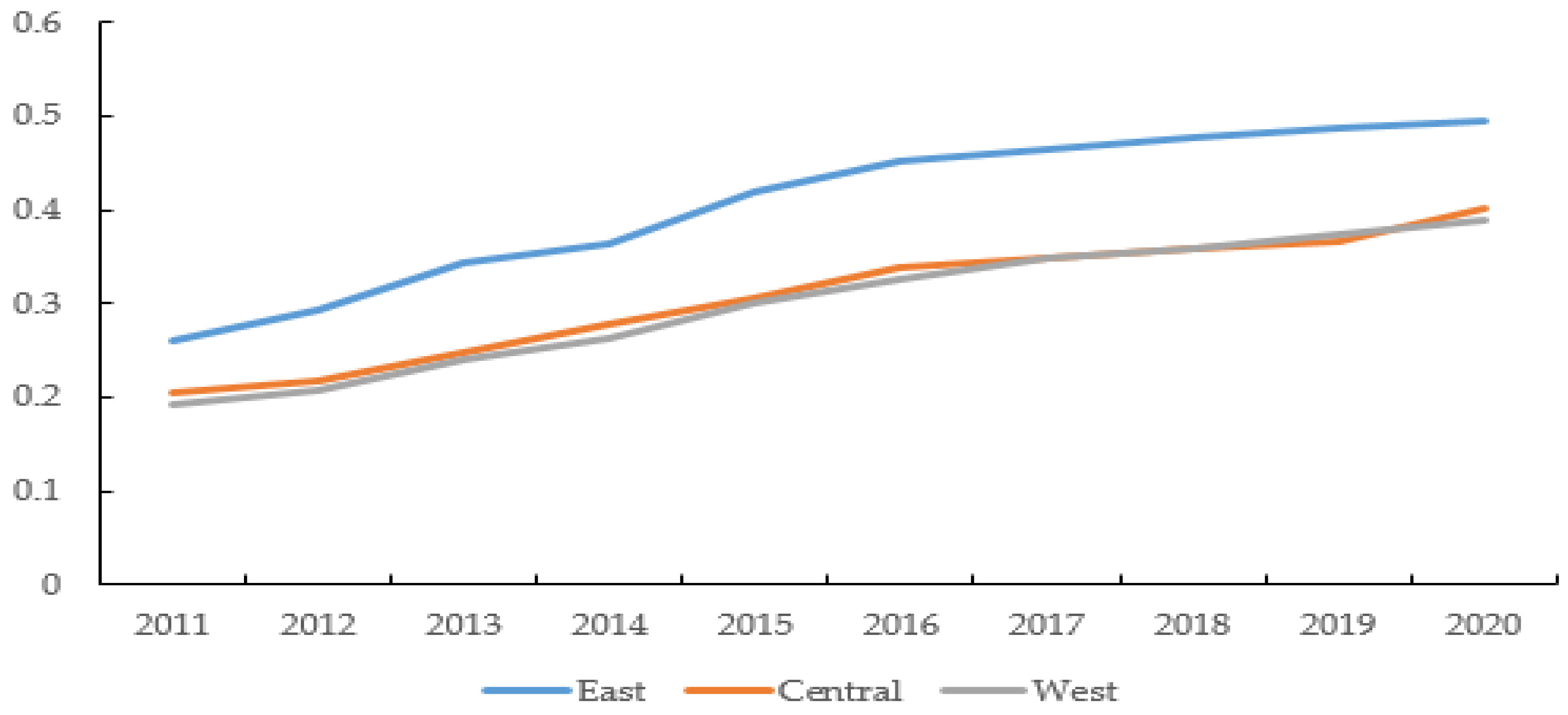
4.1. Measurement Results of GD

According to the comprehensive evaluation index system of GD constructed in Table 1, the entropy weight method was used to calculate the value of GD. The results are shown in

Table 2. Value of GD in China from 2011 to 2020.

	2011	2012	2013	2014	2015	2016	2017	2018	2019	2020	Mean
Beijing	0.2935	0.3431	0.3803	0.4092	0.4691	0.5311	0.5869	0.6002	0.6758	0.6427	0.4932
Tianjin	0.2501	0.2762	0.3338	0.3586	0.3875	0.4454	0.4144	0.4153	0.4154	0.4743	0.3771
Hebei	0.2583	0.2886	0.3513	0.3617	0.4505	0.4464	0.4154	0.4079	0.4195	0.4144	0.3814
Shanxi	0.2036	0.1963	0.2149	0.2232	0.2304	0.2325	0.2418	0.2507	0.2790	0.2821	0.2355
Inner Mongolia	0.2077	0.2232	0.2906	0.2961	0.3911	0.3789	0.3824	0.4056	0.4309	0.4956	0.3502
Liaoning	0.2521	0.2769	0.3358	0.3410	0.3720	0.3358	0.2873	0.2963	0.3048	0.2976	0.3100
Jilin	0.1674	0.1891	0.2284	0.2449	0.2067	0.2273	0.2563	0.2708	0.3048	0.3679	0.2464
Heilongjiang	0.1488	0.1374	0.1633	0.1746	0.2015	0.1974	0.2015	0.2143	0.2067	0.2253	0.1871
Shanghai	0.2749	0.2870	0.3845	0.3867	0.4447	0.4896	0.5258	0.5833	0.6397	0.6550	0.4671
Jiangsu	0.2286	0.2418	0.3397	0.3614	0.4606	0.5265	0.5322	0.5244	0.5156	0.5362	0.4267
Zhejiang	0.2566	0.2604	0.3618	0.3903	0.4763	0.5147	0.5163	0.5264	0.5355	0.5216	0.4360
Anhui	0.2871	0.2749	0.3194	0.3517	0.4186	0.4797	0.5270	0.5252	0.5224	0.5201	0.4226
Fujian	0.1850	0.2253	0.2480	0.2749	0.3162	0.3586	0.3379	0.3277	0.3369	0.3668	0.2977
Jiangxi	0.1467	0.2108	0.2056	0.2005	0.2408	0.2718	0.2769	0.2907	0.3038	0.4102	0.2558
Shandong	0.2362	0.2489	0.3242	0.3630	0.4695	0.5239	0.5419	0.5288	0.5146	0.4799	0.4231
Henan	0.2366	0.2645	0.3007	0.3751	0.4681	0.5115	0.4919	0.4896	0.5063	0.4526	0.4097
Hubei	0.2335	0.2480	0.2707	0.3007	0.3658	0.4009	0.4226	0.4153	0.4071	0.3906	0.3455
Hunan	0.2077	0.2346	0.2759	0.3441	0.3203	0.3792	0.3782	0.3836	0.4082	0.5549	0.3487
Guangdong	0.3033	0.3551	0.4109	0.4322	0.4783	0.5295	0.5318	0.5427	0.5525	0.5306	0.4667
Guangxi	0.1757	0.1808	0.2234	0.2476	0.2950	0.3479	0.3700	0.3761	0.3844	0.3851	0.2986
Hainan	0.3214	0.3834	0.2945	0.3317	0.2852	0.2811	0.4237	0.4412	0.4578	0.5167	0.3736
Chongqing	0.1602	0.1911	0.2245	0.2414	0.2930	0.3324	0.3648	0.3740	0.3855	0.3778	0.2945
Sichuan	0.2294	0.2531	0.3040	0.3344	0.3798	0.4296	0.4475	0.4759	0.5064	0.4399	0.3800
Guizhou	0.1932	0.1880	0.1955	0.2124	0.2372	0.2653	0.2935	0.3042	0.3173	0.2986	0.2505
Yunnan	0.1839	0.2025	0.2245	0.2434	0.2795	0.2983	0.3111	0.3164	0.3441	0.3546	0.2758
Shannxi	0.2718	0.2769	0.2854	0.2899	0.3281	0.3262	0.3483	0.3632	0.3803	0.3944	0.3264
Gansu	0.1819	0.1942	0.2048	0.2465	0.2775	0.3066	0.3328	0.3316	0.3328	0.3351	0.2744
Qinghai	0.1795	0.1890	0.2529	0.3062	0.2253	0.3035	0.3239	0.3032	0.3181	0.3376	0.2739
Ningxia	0.1633	0.1984	0.2286	0.2465	0.2888	0.2911	0.3348	0.3466	0.3607	0.3482	0.2777
Xinjiang	0.1746	0.1870	0.2121	0.2321	0.3033	0.2942	0.3255	0.3358	0.3483	0.4047	0.2808
Mean	0.2204	0.2409	0.2797	0.3041	0.3454	0.3752	0.3915	0.3989	0.4125	0.4270	0.3396

.

The results in

Table 3. Theil index calculation results.

Year	(1)	(2)		(3)		(4)
	$\mathit{T}$	${\mathit{T}}_{\mathit{w}}$	${\mathit{T}}_{\mathit{b}}$	${\mathit{C}}_{\mathit{w}}$	${\mathit{C}}_{\mathit{b}}$	T-East	T-Central	T-West
2011	0.0236	0.0143	0.0093	0.6057	0.3962	0.0098	0.0247	0.0123
2012	0.0255	0.0136	0.0118	0.5350	0.4632	0.0133	0.0196	0.0095
2013	0.0259	0.0118	0.0142	0.4545	0.5473	0.0080	0.0205	0.0106
2014	0.0251	0.0137	0.0114	0.5456	0.4532	0.0061	0.0336	0.0089
2015	0.0341	0.0212	0.0129	0.6220	0.3783	0.0129	0.0479	0.0130
2016	0.0370	0.0248	0.0122	0.6701	0.3303	0.0189	0.0567	0.0089
2017	0.0336	0.0236	0.0099	0.7034	0.2961	0.0201	0.0538	0.0064
2018	0.0329	0.0234	0.0096	0.7100	0.2907	0.0219	0.0461	0.0088
2019	0.0340	0.0245	0.0095	0.7200	0.2791	0.0259	0.0414	0.0104
2020	0.0284	0.0211	0.0072	0.7444	0.2544	0.0220	0.0352	0.0092

show that from 2011 to 2020, the average value of GD in China’s 30 provinces was 0.3396, and the average annual growth rate was 7.72%, indicating that China’s GD shows an upward trend. Among them, the minimum value (0.1467) appeared in Jiangxi in 2011, and the maximum value was 0.6650 in Shanghai in 2020. From an individual point of view, the green development levels represented by Beijing, Shanghai, Guangzhou, Zhejiang, and Jiangsu are relatively high, and all exceeded 0.5 in 2016. Heilongjiang, Guizhou, Qinghai, Jilin, etc., have poor GD, with the average level still below 0.3 during the sample period. The reason is that since Beijing, Shanghai, Guangzhou, Zhejiang, and other provinces are China’s developed regions, the environmental investment and residents’ living conditions are relatively high, while Heilongjiang, Guizhou, Qinghai, Jilin, and other provinces have weak economic foundations. Under the extensive management model, the backward areas are highly dependent on traditional energy and heavy industry, which has caused great damage to the ecological environment and residents’ lives. In addition, this study compared the green development in the eastern, central, and western regions as shown in Figure 3. Among them, the GD in the eastern region increased from 0.2599 to 0.4942 during the sample period, with an average growth rate of 7.54%. The central region grew from 0.2039 to 0.4004, with a growth rate of 7.85%. The western region increased from 0.1928 to 0.3897, with a growth rate of 8.21%. These evidences show that the GD in the eastern, central, and western regions has shown an increasing trend, and the growth rate in the central and western regions is higher.

4.2. Analysis of Regional Differences

To clarify the regional differences in China’s GD, this study used the Theil index to decompose the between-group differences and within-group differences in the eastern, central, and western regions. The results are shown in Table 3. Column (1) is the Theil index of the country calculated using Equation (8). Column (2) is the Theil index of the within-group difference and between-group difference calculated using Formulas (11) and (12), respectively. Column (3) is the contribution of the within-group difference and the between-group difference calculated using Equation (13). Column (4) is the intra-regional Theil index for the eastern, central, and western regions calculated using Equation (10).

The results in column (1) of Table 3 show that China’s GD has a staged developmental feature. During 2011–2020, the years with the largest and smallest such interprovincial differences occurred in 2011 and 2016, and their values were 0.0236 and 0.0370, respectively. From the changing trend, the Theil index of China’s GD has the characteristics of an inverted U shape. It continued to rise until 2016, and then it decreased. This shows that the overall gap in China’s GD is shrinking. In the results of columns (2) and (3), the Theil index within the region was consistent with the trend of the country, and it also had the characteristic stages of rising first and then falling. The Theil index within the region contributed 63% to the regional difference. The value of the Theil index between groups continued to decline, and the contribution of the inter-regional Theil index was 37%. These evidences show that the differences within the regional groups were the main source of the gaps in GD across the country. In the results of column (4), the value of the Theil index within the eastern region was between 0.0061–0.0259, the central region was between 0.0196–0.0567, and the western region was between 0.0064–0.0130. These evidences show that there were also large gaps in GD within each region. Among them, the gap within the eastern and western regions was smaller, and the gap within the central region was the largest. Overall, the calculation results of the Theil index show that there are large regional differences in China’s GD, and the differences within the regional groups are the main source for the overall differences in China’s GD. At the same time, there are also large differences within each region, and the GD within the central region is the most unbalanced.

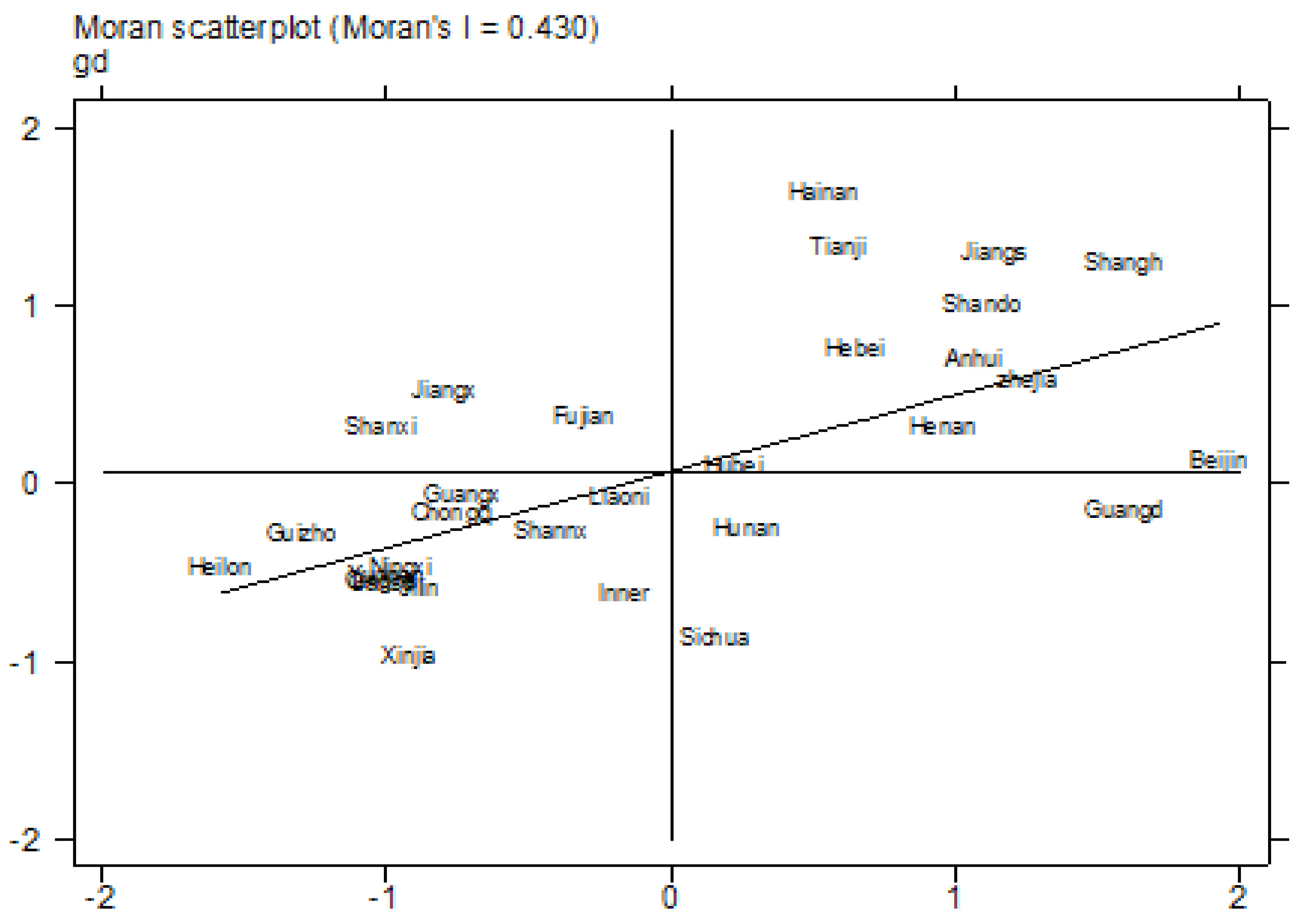
4.3. Spatial Dynamic Convergence Analysis

The decomposition results of the Theil index show the static differences of the regional GD in China. To clarify the spatial dynamic evolution trend of the regional GD, this study used the spatial β-convergence model to test the convergence of the regional GD. Using a spatial economic model requires testing the spatial correlation of variables. This study used the spatial Moran index (Moran’s I) to test the regional relevance of GD in 30 provinces. The Moran’s I is calculated as shown in Equation (18).

$$I=\frac{{\displaystyle \sum _{i=1}^n{\displaystyle \sum _{j=1}^n{W}_{ij}}(g{d}_i-\overline{gd}})(g{d}_j-\overline{gd})}{S^2{\displaystyle \sum _{i=1}^n{\displaystyle \sum _{j=1}^n{W}_{ij}}}}$$

(18)

In Equation (18), $S^2=\frac{1}{n}{{\displaystyle \sum _{i=1}^n\left(g{d}_i-\overline{gd}\right)}}^2$. $g{d}_i$ and $g{d}_j$ are the values of GD in the i and j provinces, respectively, and $\overline{gd}$ is the average value. $W$ is the spatial weight matrix. Moran’s I was [−1, 1]. When it is positive, the GD in adjacent areas has a significant positive correlation.

Table 4. Results of the calculation of Moran’s I.

Year	Moran’s I	Z Statistic
2011	0.184 *	1.793
2012	0.196 **	2.092
2013	0.225 **	2.357
2014	0.216 **	2.268
2015	0.307 ***	3.083
2016	0.361 ***	3.563
2017	0.378 ***	3.732
2018	0.328 ***	3.288
2019	0.273 ***	2.813
2020	0.288 ***	2.944

Note: ***, **, and * represent the significance of the Z values at 1%, 5%, and 10%, respectively.

shows the calculation results of the Moran index.

The results in Table 4 show that between 2011 and 2020, the Moran’s I was between 0.184 and 0.378, showing an overall upward trend. This indicated a positive spatial correlation of GD in China. Therefore, the spatial economic models can be used for research. In addition, Figure 4 shows a scatter plot of the local Moran index of green development in 30 provinces. The results show that many provinces are in the first and third quadrants, representing the spatial characteristics of GD with high–high aggregation and low–low aggregation.

After confirming the rationality of the spatial economic model, this study continued to use the spatial β-convergence model to test the convergence of GD. At the same time, this study used the Lagrange multiplier test (LM-test) to test the fitness of the SAR and SEM models. The results show that the LM-Lag statistic value was 2.85, which failed the significance test. The LM-Error and robust LM-Error statistics were 117.36 and 35.88 and were significant at the 1% level, which indicated that the SEM model was more suitable. In addition, the Hausman test’s result (Prob>chi2 = 0.0000) rejected the random-effects null hypothesis, which indicated that the model selection of fixed effects was more effective.

Table 5. Spatial absolute β-convergence of GD.

	(1)	(2)	(3)	(4)
	All	East	Central	West
β	−0.356 **	−0.446 **	−0.302 ***	−0.362 **
	(−2.13)	(−2.09)	(−3.35)	(−2.01)
λ	0.214 **	0.236 ***	0.198 **	0.259 **
	(2.12)	(3.11)	(2.16)	(2.29)
s	0.044	0.059	0.036	0.045
T	15.753	11.748	19.254	15.403
N	300	110	80	110
R2	0.183	0.142	0.114	0.131

Note: *** and ** represent the significance of the p values at 1% and 5%, respectively.

is the calculated spatial absolute β-convergence using Equations (14) and (15). Column (1) shows the calculation results for the whole country, and columns (2), (3), and (4) are those of the eastern, central, and western regions, respectively.

Table 6. Spatial conditional β-convergence of GD.

	(1)	(2)	(3)	(4)
	All	East	Central	West
β	−0.462 **	−0.513 **	−0.457 **	−0.483 **
	(−2.25)	(−2.12)	(−2.41)	(−2.20)
gp	0.328 ***	0.274 **	0.359 **	0.327 **
	(2.91)	(2.20)	(2.41)	(2.26)
λ	0.217 **	0.241 ***	0.199 **	0.260 **
	(2.13)	(2.99)	(2.15)	(2.27)
s	0.062	0.072	0.061	0.066
T	11.180	9.627	11.363	10.502
N	300	110	80	110
R2	0.191	0.164	0.137	0.153

Note: *** and ** represent the significance of the p values at 1% and 5%, respectively.

shows the convergence of the spatial condition β, calculated using Equations (16) and (17). Column (1) shows the calculation results for the whole country, and columns (2), (3) and (4) are those of the eastern, central, and western regions, respectively.

In Table 5, the β-convergence coefficient of GD across the country is significantly negative at the 5% level, which indicates that the GD of each province had the characteristics of absolute β-convergence; that is, provinces with a low level of GD will catch up with those with a high level and eventually reach a steady state. From the perspective of the three regions, the β-convergence coefficients of the three regions are all significantly negative, which indicates that the green development in the three regions also had the characteristics of absolute β-convergence, and there was a common steady state among the provinces within the region. In addition, comparing the convergence speed(s), we found significant differences between the regions, with the eastern region having the fastest convergence speed, and the central region having the slowest convergence speed. This is due to the green development of the central provinces being quite different, resulting in a slow convergence to the steady state.

The results in Table 6 show that the β-convergence coefficients are all less than 0 in the whole country or in the three regions, and they are all significant at the 5% level, indicating that China’s GD has the obvious characteristics of conditional β-convergence. From the perspective of the conditional β-convergence speed, the conditional β-convergence rate in the whole country and in the eastern and western regions are still higher. However, when comparing the absolute β-convergence speed, we found that the convergence speed of each region increased significantly. The gap between the central region and other regions is also shrinking, indicating that the GD of various regions in China has finally converged to a steady state, and the narrowing of the gap between the central region and the east–west convergence speed also reflects the “catch-up effect” within the central region. In addition, the coefficient of green innovation is significantly positive, which indicates that green innovation is conducive to promoting the convergence of regional GD and effectively reduces the convergence speed of regional GD.

4.4. Discussion

Green development is important for economic sustainability, environmental sustainability, and social sustainability. Based on the green development evaluation system of the three dimensions of the economy, environment, and society, this study identified the differences and convergence of China’s green development. First, the average value of China’s green development from 2011 to 2020 was 0.3396, showing a rising trend, which is lower than the results of GTFP based on the economic efficiency and environmental efficiency [54,55]. The results are lower because our study also considered the impact of social efficiency indicators such as green life, social equity, and residents’ environmental satisfaction on green development, which makes our calculation results more extensive and more scientific. Second, China’s GD has great regional differences, and these regional differences present a phased characteristic of rising first and then falling. Among them, the differences of GD within the eastern and western regions are relatively smaller, and the central region is the largest. The average contribution to the within-group difference was 63%, which indicated that the within-group differences were the main source of the GD gaps. Compared with ordinary empirical analysis, the analysis of the difference and contribution in this study can more scientifically show the characteristics of China’s GD [32,56]. Finally, China’s GD has obvious characteristics of spatial absolute β-convergence and spatial conditional β-convergence, and the GD of each province tends to a common steady state. Among them, the eastern region has the fastest convergence speed, and the central region has the slowest convergence speed. Under the influence of green innovation, the convergence speed between the central region and other regions is shrinking, which indicates that green innovation can promote the steady-state convergence of GD within the central region. The analysis based on spatial convergence clearly shows the characteristics of the spatial evolution of China’s regional GD, which can make up for the lack of research on the dynamic evolution trend of GD [33].

5. Conclusions and Policy Implications

This study constructed a GD evaluation system based on the three dimensions of the economy, environment, and society. First, the entropy method was used to measure the GD in 30 provinces in China from 2011 to 2020. Second, the Theil index decomposition method was used to analyze the regional differences and contributions of GD. Finally, the spatial β-convergence model was used to test the spatial evolution characteristics of China’s regional GD. The research results are as follows. First, the comprehensive evaluation results show that the average GD of China’s 30 provinces from 2011 to 2020 was 0.3396, with an average annual growth rate of 7.72%. The GD in the eastern region increased from 0.2599 to 0.4942 during the sample period, with an average growth rate of 7.54%. The central region grew from 0.2039 to 0.4004, with a growth rate of 7.85%. The western region increased from 0.1928 to 0.3897, with a growth rate of 8.21%. This evidence shows that China’s regional GD has an upward trend and that the eastern region is higher. Second, the Theil index calculation results show that from 2011 to 2020, the years with the largest and smallest regional gaps in China’s green development occurred in 2011 and 2016, which were 0.0236 and 0.0370, respectively. The regional differences of China’s GD have the characteristic of rising first and then falling. At the same time, the Theil index decomposition results show that the contribution rate of the Theil index within the region was 63% and that the contribution rate between regions was 37%, which indicates that the differences within regions are the main source of imbalances in China’s GD. Third, the β coefficient in the regression results of the spatial convergence model is significantly negative, and the coefficient of green innovation is significantly positive. These evidences show that China’s GD has the obvious characteristics of spatial absolute β-convergence and spatial conditional β-convergence and that green innovation is conducive to narrowing the gaps in the convergence speed of regional GD.

To achieve the goal of GD more scientifically, the policy implications are as follows. First, the GD is a comprehensive index that takes into account the economic, environmental, social, and other aspects. It is different from the evaluation of economic growth or ecological quality under single-dimensional indicators; the social effect of GD is indispensable. In the implementation of GD policies, the government needs to strengthen the coordination of the economy, environment, and society. On one hand, it is imperative to change the extensive model of economic growth with high consumption and high pollution and transform it into a sustainable development model with low consumption, low emissions, and high technology; improve the utilization efficiency of resources; and reduce pollution emissions. On the other hand, it is also necessary to adhere to people-oriented factors, pay attention to social equity, and improve the quality and satisfaction of residents’ green life. Second, the key to solving the imbalance in China’s GD is to narrow the differences within regions. For regions with a low level of GD, the government should provide active fiscal and taxation policies to provide development space for their green transformation. The local governments also need to formulate more precise stage goals for green development and formulate differentiated regional green development plans according to the actual conditions of each province. Third, it is necessary to strengthen the spatial interaction of GD among provinces and give opportunities for the positive role of green technology innovation. In the process of regional GD, it is necessary to strengthen the cooperation between adjacent regions, give opportunities for the comparative advantages of each region, build a green technology research and development platform for cross-regional cooperation, improve the sharing of regional resources and technologies, and provide opportunities for backward provinces to catch up with developed regions.

The research on the differences and convergence in this study is helpful for a more comprehensive and in-depth understanding of the regional characteristics and evolutionary dynamics of China’s GD, but there are still limitations. Due to the difficulty of data acquisition, this study selected research samples from 30 provinces in China, but the research based on urban and rural GD will be the focus of our future research. In addition, this study selected the evaluation indicators of GD from the three dimensions of the economy, environment, and society as much as possible, but the changes of indicators will cause uncertainty in the evaluation results. As government policies and residents’ needs change, the index system of this study can be further enriched and optimized.

References

1. Singh, S.; Upadhyay, S.P.; Powar, S. Developing an integrated social, economic, environmental, and technical analysis model for sustainable development using hybrid multi-criteria decision making methods. Appl. Energy 2022, 308, 118235. [Google Scholar] [CrossRef]
2. Chatzistamoulou, N.; Tyllianakis, E. Green growth & sustainability transition through information. Are the greener better informed? Evidence from European SMEs. J. Environ. Manag. 2022, 306, 114457. [Google Scholar] [CrossRef]
3. Debbarma, J.; Choi, Y. A taxonomy of green governance: A qualitative and quantitative analysis towards sustainable development. Sustain. Cities Soc. 2022, 79, 103693. [Google Scholar] [CrossRef]
4. Fang, G.; Wang, Q.; Tian, L. Green development of Yangtze River Delta in China under Population-Resources-Environment-Development-Satisfaction perspective. Sci. Total Environ. 2020, 727, 138710. [Google Scholar] [CrossRef] [PubMed]
5. Brust, D.V.; Smith, A.M.; Sarkis, J. Managing the transition to critical green growth: The ‘Green Growth State’. Futures 2014, 64, 38–50. [Google Scholar] [CrossRef]
6. Wang, Y.; Chen, H.; Long, R.; Sun, Q.; Jiang, S.; Liu, B. Has the Sustainable Development Planning Policy Promoted the Green Transformation in China’s Resource-based Cities? Resour. Conserv. Recycl. 2022, 180, 106181. [Google Scholar] [CrossRef]
7. Bhutta, U.S.; Tariq, A.; Farrukh, M.; Raza, A.; Iqbal, M.K. Green bonds for sustainable development: Review of literature on development and impact of green bonds. Technol. Forecast. Soc. Change 2022, 175, 121378. [Google Scholar] [CrossRef]
8. Sarwar, S. Impact of energy intensity, green economy and blue economy to achieve sustainable economic growth in GCC countries: Does Saudi Vision 2030 matters to GCC countries. Renew. Energy 2022, 191, 30–46. [Google Scholar] [CrossRef]
9. D’Amato, D.; Korhonen, J. Integrating the green economy, circular economy and bioeconomy in a strategic sustainability framework. Ecol. Econ. 2021, 188, 107143. [Google Scholar] [CrossRef]
10. Ringel, M.; Schlomann, B.; Krail, M.; Rohde, C. Towards a green economy in Germany? The role of energy efficiency policies. Appl. Energy 2016, 179, 1293–1303. [Google Scholar] [CrossRef]
11. Orlov, S.; Rovenskaya, E. Optimal transition to greener production in a pro-environmental society. J. Math. Econ. 2022, 98, 102554. [Google Scholar] [CrossRef]
12. Muhammad, S.; Pan, Y.; Agha, M.H.; Umar, M.; Chen, S. Industrial structure, energy intensity and environmental efficiency across developed and developing economies: The intermediary role of primary, secondary and tertiary industry. Energy 2022, 247, 123576. [Google Scholar] [CrossRef]
13. Nepal, R.; Paija, N.; Tyagi, B.; Harvie, C. Energy security, economic growth and environmental sustainability in India: Does FDI and trade openness play a role? J. Environ. Manag. 2021, 281, 111886. [Google Scholar] [CrossRef]
14. Hou, S.; Song, L. Market integration and regional green total factor productivity: Evidence from China’s province-Level Data. Sustainability 2021, 13, 472. [Google Scholar] [CrossRef]
15. Zhao, P.; Gao, Y.; Sun, X. How does artificial intelligence affect green economic growth?—Evidence from China. Sci. Total Environ. 2022, 834, 155306. [Google Scholar] [CrossRef] [PubMed]
16. Attahiru, Y.B.; Aziz, M.; Kassim, K.A.; Shahid, S. A review on green economy and development of green roads and highways using carbon neutral materials. Renew. Sustain. Energy Rev. 2019, 101, 600–613. [Google Scholar] [CrossRef]
17. Hafezi, M.; Zolfagharinia, H. Green product development and environmental performance: Investigating the role of government regulations. Int. J. Prod. Econ. 2018, 204, 395–410. [Google Scholar] [CrossRef]
18. Verbeek, T.; Hincks, S. The ‘just’ management of urban air pollution? A geospatial analysis of low emission zones in Brussels and London. Appl. Geogr. 2022, 140, 102642. [Google Scholar] [CrossRef]
19. Kalaitzoglou, I.; Ibrahim, B.M. Trading patterns in the European carbon market: The role of trading intensity and OTC transactions. Q. Rev. Econ. Financ. 2013, 53, 402–416. [Google Scholar] [CrossRef]
20. Javeed, S.A.; Latief, R.; Jiang, T.; Ong, T.; Tang, Y. How environmental regulations and corporate social responsibility affect the firm innovation with the moderating role of Chief executive officer (CEO) power and ownership concentration? J. Clean. Prod. 2021, 308, 127212. [Google Scholar] [CrossRef]
21. Habiba, U.; Cao, X.; Anwar, A. Do green technology innovations, financial development, and renewable energy use help to curb carbon emissions? Renew. Energy 2022, 193, 1082–1093. [Google Scholar] [CrossRef]
22. Chawla, S.; Rai, P.; Garain, T.; Uday, S.; Hussain, C.M. Green Carbon Materials for the Analysis of Environmental Pollutants. Trends Environ. Anal. Chem. 2022, 33, e00156. [Google Scholar] [CrossRef]
23. D’Amato, A.; Mazzanti, M.; Nicolli, F. Green technologies and environmental policies for sustainable development: Testing direct and indirect impacts. J. Clean. Prod. 2021, 309, 127060. [Google Scholar] [CrossRef]
24. Erdogan, S. Dynamic Nexus between Technological Innovation and Building Sector Carbon Emissions in the BRICS Countries. J. Environ. Manag. 2021, 293, 112780. [Google Scholar] [CrossRef]
25. Khan, I.; Zakari, A.; Dagar, V.; Singh, S. World energy trilemma and transformative energy developments as determinants of economic growth amid environmental sustainability. Energy Econ. 2022, 108, 105884. [Google Scholar] [CrossRef]
26. Li, W.; Yi, P. Assessment of city sustainability—Coupling coordinated development among economy, society and environment. J. Clean. Prod. 2020, 256, 120453. [Google Scholar] [CrossRef]
27. Herrero, C.; Pineda, J.; Villar, A.; Zambrano, E. Tracking progress towards accessible, green and efficient energy: The Inclusive Green Energy index. Appl. Energy 2020, 279, 115691. [Google Scholar] [CrossRef]
28. Simarro, R.M. Inequality in China revisited. The effect of functional distribution of income on urban top incomes, the urban-rural gap and the Gini index, 1978–2015. China Econ. Rev. 2017, 42, 101–117. [Google Scholar] [CrossRef]
29. Branis, M.; Linhartova, M. Association between unemployment, income, education level, population size and air pollution in Czech cities: Evidence for environmental inequality? A pilot national scale analysis. Health Place 2012, 18, 1110–1114. [Google Scholar] [CrossRef]
30. Giaccherini, M.; Kopinska, J.; Palma, A. When particulate matter strikes cities: Social disparities and health costs of air pollution. J. Health Econ. 2021, 78, 102478. [Google Scholar] [CrossRef]
31. Jing, Z.; Wang, J. Sustainable development evaluation of the society–economy–environment in a resource-based city of China: A complex network approach. J. Clean. Prod. 2020, 263, 121510. [Google Scholar] [CrossRef]
32. Yang, Y.; Guo, H.; Chen, L.; Liu, X.; Gu, M.; Ke, X. Regional analysis of the green development level differences in Chinese mineral resource-based cities. Resour. Policy 2019, 61, 261–272. [Google Scholar] [CrossRef]
33. Gao, K.; Yuan, Y. Spatiotemporal pattern assessment of China’s industrial green productivity and its spatial drivers: Evidence from city-level data over 2000–2017. Appl. Energy 2022, 307, 118248. [Google Scholar] [CrossRef]
34. Development and Reform Commission of China (DRCC). The Development and Reform Commission of China Issued “the Green Development Index System” and “Ecological Civilization Construction Assessment Target System”. 2016. Available online: http://www.gov.cn/xinwen/2016-12/22/content_5151575.htm (accessed on 5 May 2022).
35. Koengkan, M.; Fuinhas, J.A.; Kazemzadeh, E.; Osmani, F. Measuring the economic efficiency performance in Latin American and Caribbean countries: An empirical evidence from stochastic production frontier and data envelopment analysis. Int. Econ. 2022, 169, 43–54. [Google Scholar] [CrossRef]
36. Silva, P.M.; Moutinho, V.F.; Moreira, A.C. Do social and economic factors affect the technical efficiency in entrepreneurship activities? Evidence from European countries using a two-stage DEA model. Socio-Econ. Plan. Sci. 2022, 82, 101314. [Google Scholar] [CrossRef]
37. Wang, R.; Qi, Z.; Shu, Y. Multiple relationships between fixed-asset investment and industrial structure evolution in China–Based on Directed Acyclic Graph (DAG) analysis and VAR model. Struct. Change Econ. Dyn. 2020, 55, 222–231. [Google Scholar] [CrossRef]
38. Llop, M. Economic structure and pollution intensity within the environmental input–output framework. Energy Policy 2007, 35, 3410–3417. [Google Scholar] [CrossRef]
39. Namazi, M.; Mohammadi, E. Natural resource dependence and economic growth: A TOPSIS/DEA analysis of innovation efficiency. Resour. Policy 2018, 59, 544–552. [Google Scholar] [CrossRef]
40. Vamza, I.; Kubule, A.; Zihare, L.; Valters, K.; Blumberga, D. Bioresource utilization index–A way to quantify and compare resource efficiency in production. J. Clean. Prod. 2021, 320, 128791. [Google Scholar] [CrossRef]
41. Aminzadegan, S.; Shahriari, M.; Mehranfar, F.; Abramović, B. Factors affecting the emission of pollutants in different types of transportation: A literature review. Energy Rep. 2022, 8, 2508–2529. [Google Scholar] [CrossRef]
42. Keyser, W.; Gevaert, V.; Verdonck, F.; Baets, B.; Benedetti, L. An emission time series generator for pollutant release modelling in urban areas. Environ. Model. Softw. 2010, 25, 554–561. [Google Scholar] [CrossRef]
43. Pillay, Y.P.; Buschke, F.T. Misaligned environmental governance indicators and the mismatch between government actions and positive environmental outcomes. Environ. Sci. Policy 2020, 112, 374–380. [Google Scholar] [CrossRef]
44. Chu, Z.; Bian, C.; Yang, J. How can public participation improve environmental governance in China? A policy simulation approach with multi-player evolutionary game. Environ. Impact Assess. Rev. 2022, 95, 106782. [Google Scholar] [CrossRef]
45. Dugoua, E.; Dumas, M. Green product innovation in industrial networks: A theoretical model. J. Environ. Econ. Manag. 2021, 107, 102420. [Google Scholar] [CrossRef]
46. Filippini, M.; Obrist, A. Are households living in green certified buildings consuming less energy? Evidence from Switzerland. Energy Policy 2022, 161, 112724. [Google Scholar] [CrossRef]
47. Shafique, M.; Luo, X. Environmental life cycle assessment of battery electric vehicles from the current and future energy mix perspective. J. Environ. Manag. 2022, 303, 114050. [Google Scholar] [CrossRef]
48. Jones, B.A. Planting urban trees to improve quality of life? The life satisfaction impacts of urban afforestation. For. Policy Econ. 2021, 125, 102408. [Google Scholar] [CrossRef]
49. Omri, A.; Omri, H.; Slimani, S.; Belaid, F. Environmental degradation and life satisfaction: Do governance and renewable energy matter? Technol. Forecast. Soc. Change 2022, 175, 121375. [Google Scholar] [CrossRef]
50. Vega, C.; Volij, O. A simple proof of Foster’s (1983) characterization of the Theil measure of inequality. Econ. Model. 2013, 35, 940–943. [Google Scholar] [CrossRef] [Green Version]
51. Barro, R.; Martin, X.S. Convergence. J. Polit. Econ. 1992, 100, 223–251. [Google Scholar] [CrossRef]
52. Francisco, A.; Sosa, C.; Cabral, R.; Mollick, A.V. Energy reform and energy consumption convergence in Mexico: A spatial approach. Struct. Change Econ. Dyn. 2022, 61, 336–350. [Google Scholar] [CrossRef]
53. Losacker, S. ‘License to green’: Regional patent licensing networks and green technology diffusion in China. Technol. Forecast. Soc. Chang. 2022, 175, 121336. [Google Scholar] [CrossRef]
54. Xia, F.; Xu, J. Green total factor productivity: A re-examination of quality of growth for provinces in China. China Econ. Rev. 2020, 62, 101454. [Google Scholar] [CrossRef]
55. Zhai, X.; Xue, R.; He, B.; Yang, D. Dynamic changes and convergence of China’s regional green productivity: A dynamic spatial econometric analysis. Adv. Clim. Chang. Res. 2022, 13, 266–278. [Google Scholar] [CrossRef]
56. Huang, H.; Mo, R.; Chen, X. New patterns in China’s regional green development: An interval Malmquist–Luenberger productivity analysis. Struct. Chang. Econ. Dyn. 2021, 58, 161–173. [Google Scholar] [CrossRef]
Figure 1. China’s regional status in 2010–2020 (sample period mean).
Sustainability 14 08511 g001
Figure 2. System framework of green development.
Sustainability 14 08511 g002
Figure 3. Regional green development from 2011 to 2020.
Sustainability 14 08511 g003
Figure 4. Scatter plot of local Moran’s I.
Sustainability 14 08511 g004