Total Variation-Based Metrics for Assessing Complementarity in Energy Resources Time Series

Abstract

The growing share of intermittent renewable energy sources raised complementarity to a central concept in the electricity supply industry. The straightforward case of two sources suggests that to guarantee supply, the time series of both sources should be negatively correlated. Extrapolation made Pearson’s correlation coefficient ($\rho$) the most widely used metric to quantify complementarity. This article shows several theoretical and practical drawbacks of correlation coefficients to measure complementarity. Consequently, it proposes three new alternative metrics robust to those drawbacks based on the natural interpretation of the concept: the Total Variation Complementarity Index ($\varphi$), the Variance Complementarity Index (${\varphi }^{\prime }$), and the Standard Deviation Complementarity Index (${\varphi }_s$). We illustrate the use of the three indices by presenting one theoretical and three real case studies: (a) two first-order autoregressive processes, (b) one wind and one hydropower energy time series in Colombia at the daily time resolution, (c) monthly water inflows to two hydropower reservoirs of Colombia with different hydrologic regimes, and (d) monthly water inflows of the 15 largest hydropower reservoirs in Colombia. The conclusion is that $\varphi$ outperforms the use of $\rho$ to quantify complementarity because (i) $\varphi$ takes into account scale, whereas $\rho$ is insensitive to scale; (ii) $\rho$ does not work for more than two sources; (iii) $\rho$ overestimates complementarity; and (iv) $\varphi$ takes into account other characteristics of the series. ${\varphi }^{\prime }$ corrects the scale insensitivity of $\rho$. Moreover, it works with more than two sources. However, it corrects neither the overestimation nor the importance of other characteristics. ${\varphi }_s$ improves ${\varphi }^{\prime }$ concerning the overestimation, but it lets out other series characteristics. Therefore, we recommend total variation complementarity as an integral way of quantifying complementarity.

1. Introduction

The proliferation of energy sources made possible by technological advances and consequent cost reduction introduced the term complementarity into the energy jargon. Most of those new sources have a large natural variability.

The concept of complementarity is of particular interest when the resource’s availability or costs are variable in time. Despite the lack of a formal definition, intuition suggests that complementarity refers to the possibility of using different resources according to their availability to meet a given demand. However, each one separately accounts for only a fraction of the demand.

Correlation coefficients are by far the most widely used metric for assessing complementarity between energy sources’ time series. This approach has been used, for example, in Poland [1], Portugal [2,3], Spain [4], Italy [5,6], USA [7], Germany [8], Australia [9], Brazil [10,11,12,13], China [14,15,16], Sweden [17], Mexico [18], Canada [19], Lesotho [20], Finland [21], Argentina [22], Britain [23], Saudi Arabia [24], and Chile [25]. It has also been used at the international level (e.g., Latin America [26], Iberian Peninsula [27]), and even at the intercontinental level (e.g., Canada vs. Noruega [19] and Europe vs. Africa [28]).

In the case of Colombia, Pearson’s correlation coefficient has been the most used metric [29,30,31,32,33,34,35,36]. Paredes and Ramírez [30] concluded that the highest negative mean seasonal R coefficients were at the wind and solar sites on the Oriental Plains and solar sites in the Antioquia region. They also found seasonal complementarity between wind sites in the north and east and northern rivers, between wind sites in the south and center and the rivers there, and between north and east solar sites and northern rivers. Henao et al. [34] found that solar and wind resources in the Caribbean Coast and the central Andes regions can complement the country’s hydropower sector during the dry seasons of the annual climatological cycle and ENSO events. Peña Gallardo et al. [32] concluded that there is good energetic complementarity in the north and northeastern regions of the country throughout the year. Parra et al. [33] concluded that the Colombian power system evidenced an overall low complementarity behavior between its renewable power plants. This low complementarity indicates that most hydro-based power plants present similar temporal and amplitude characteristics, making the power system vulnerable to droughts. Wind and solar power plants have a high potential to complement Colombia’s hydroelectric system, suggesting that more power capacity is needed to enhance such complementarity.

Under this approach, there is a high complementarity between two resources when their time series have a high negative correlation coefficient, sometimes called anticorrelation (e.g., [7,16,23,27,28]).

However, a complementarity metric should measure the regularity of the sum of all available resources, and correlation coefficients fail to accomplish that. The use of correlation coefficients also has the following issues, also presented by us in Cantor et al. [36]:

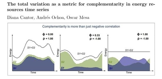
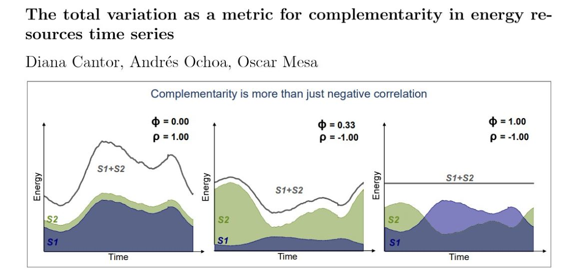
• Negative correlation is not complementarity. Although complementarity entails negative correlation, negative correlation does not entail complementarity. For example, the correlation between speed and height in a pendulum is negative, but they are not complementary.
• Dimensions matter. In the above example, speed and height have different units. Obviously, for two or more variables to complement, they must have the same dimension. If they have different dimensions, one cannot sum them, and their complementarity has no sense. In the pendulum example above, the complementary variables are kinetic energy and potential energy.
• The scale of the variables does matter. For example, streamflows from a large river and a small creek could exhibit a sizable negative correlation, but the large one dominates their sum. Hence, the complementarity value could be small.
• Linearity of the relation is also an issue. Even if correlation coefficients were suitable for assessing complementarity, selecting Pearson’s, Kendall’s, Spearman’s, or any other coefficient needs a physical or mathematical justification.
• It is natural to consider the complementarity of more than two resources, but a satisfactory correlation analysis is limited to two series.

Besides correlation, among the other metrics used to evaluate complementarity, one can mention the one proposed by Beluco et al. [37] as the product of three partial indices: (i) partial time complementarity index, which evaluates the time interval between the minimum values of two sources; (ii) partial energy complementarity index, which evaluates the relationship between the average values of two sources; (iii) partial amplitude-complementarity index, which assesses the differences between maximum and minimum values of the two energy sources. This idea works well for simple annual sinusoidal series but fails for more complicated series. Borba and Brito [38] proposed the dimensionless ratio between the actual generation discarding excess power and the average generation. This index is more a measure of volatility than complementarity. Han et al. [39] presented two indices of the complementary rate of fluctuation (CROF) and complementary rate of the ramp (CROR) to analyze the complementary degree of sequences with different fluctuation characteristics. Their rate of fluctuation seems to follow the concept of total variation that we present. Neto et al. [40] used the concept of Daily Physical Guarantee (DPG), similar to firm power, to evaluate different renewable energy sources’ complementarity. The general idea is interesting but depends on the system’s characteristics and does not provide a direct complementarity metric. A method was introduced in [29,41] that assesses temporal complementarity between three variable energy sources, using a combination of correlation coefficients, Euclidean vectors, compromise programming, and normalization. The method’s basis is correlation analysis, and therefore their proposal shares the criticism we made above. For a complete review of different methods to evaluate complementarity, see [42]. In our opinion, none of these metrics are satisfactory enough to assess complementarity.

This paper proposes three novel indices based on the mathematical concept of Total Variation to solve these issues (see Section 2). Conceptually, the total variation of a time series is the sum of all the changes in the series. A constant series has a total variation of zero. Therefore, a total variation of zero serves as the standard of regularity. Measuring the deviation of a sum from that standard is the motivation for defining complementarity. The other two indices use the same idea but with variance or standard deviation instead of the total variation. To illustrate the use and properties of the new indices, we apply them to four cases of study (Section 3): (1) two autoregressive processes; (2) wind vs. hydro in the Colombian electricity market; (3) two hydropower sources in the Colombian electricity market; (4) fifteen hydropower sources in the Colombian electricity market.

2. Materials and Methods

In ordinary language, two things complement each other when their combination is complete or perfect. To complement is to add to something in a way that enhances or improves it. In math, two numbers complement each other when their sum is constant, usually 1 or 100. A measure of complementarity between two functions should assess the perfection of their sum. For perfection, here, one takes the regularity of the sum. Therefore, the measure of complementarity is related to the measure of regularity. A convenient way of measuring the regularity of a function is through its total variation, which allows for simple discontinuities. It has more satisfactory properties than the variance [43] (p. 328) [44] (p. 140).

Section 2.1 reviews the concept and main mathematical properties of Total Variation. Then, Section 2.2, Section 2.3 and Section 2.4 propose indices, $\varphi$, ${\varphi }^{\prime }$, and ${\varphi }_s$ as novel metrics of complementarity. Afterward, Section 3.1, Section 3.2 and Section 3.3 present one theoretical and three real case studies to evaluate the suitability of $\varphi$ and ${\varphi }^{\prime }$ to quantify complementarity: (1) two AR(1) processes, (2) daily wind and hydropower generation time series in Colombia, (3) the daily inflows to two hydropower reservoirs in Colombia, and (4) monthly water inflows of the 15 largest hydropower reservoirs in Colombia. Results are compared between the indices. Section 3.4 presents the application of the $\varphi$ index for the evaluation of the complementarity of multiple time series.

2.1. Total Variation

According to [43,44], the total variation of a function f defined on an interval $[a,b]$ is

$$\underset{a}{\overset{b}{\bigvee }}f=sup\sum _{i=1}^n|f\left(t_i\right)-f\left(t_{i-1}\right)|,$$

(1)

where the supremum is taken over all possible finite partitions $a=t_1<\dots <t_n=b$ of $[a,b]$.

If the total variation is bounded (finite), f is said to be of bounded variation on $[a,b]$. Functions of bounded variations may have only removable discontinuities (jumps). Some important properties of the total variation are worth recalling [43]:

• The total variation of a constant function is zero, and conversely, if ${\bigvee }_a^{b}f=0$ then f is constant on $[a,b]$.
• The total variation of a monotonic function f on $[a,b]$ is $\left|f\right(b)-f(a\left)\right|$.
• ${\bigvee }_a^b\left(\alpha f\right)=\left|\alpha \right|{\bigvee }_a^b\left(f\right)$ for any constant $\alpha$.
• If $f_1$ and $f_2$ are functions of bounded variation, then so is $f_1+f_2$, and

  $$\underset{a}{\overset{b}{\bigvee }}(f_1+f_2)\le \underset{a}{\overset{b}{\bigvee }}\left(f_1\right)+\underset{a}{\overset{b}{\bigvee }}\left(f_2\right)$$

  (2)
• If $a<b<c$ then

  $$\underset{a}{\overset{c}{\bigvee }}\left(f\right)=\underset{a}{\overset{b}{\bigvee }}\left(f\right)+\underset{b}{\overset{c}{\bigvee }}\left(f\right).$$

  (3)

From the above properties, it is clear that the total variation of a function f with values $f\left(t_k\right)$ at the points $a=t_0<t_1<\dots <t_n=b$, and linear interpolation in between the given points is

$$\underset{a}{\overset{b}{\bigvee }}\left(f\right)=\sum _{k=0}^{n-1}|f\left(t_{k+1}\right)-f\left(t_k\right)|.$$

(4)

This property is useful to compute the total variation of a time series.

To illustrate, consider the following sequence of functions in $[0,1]$: $g_n\left(t\right)=sin\left(2\pi nt\right),$$n\ge 1$. Clearly, all the functions have zero mean and their variance is $1/2$, but ${\bigvee }_0^1\left(g_n\right)=4n$ [44].

Using the definition of Total Variation, it is natural to define the following complementarity index.

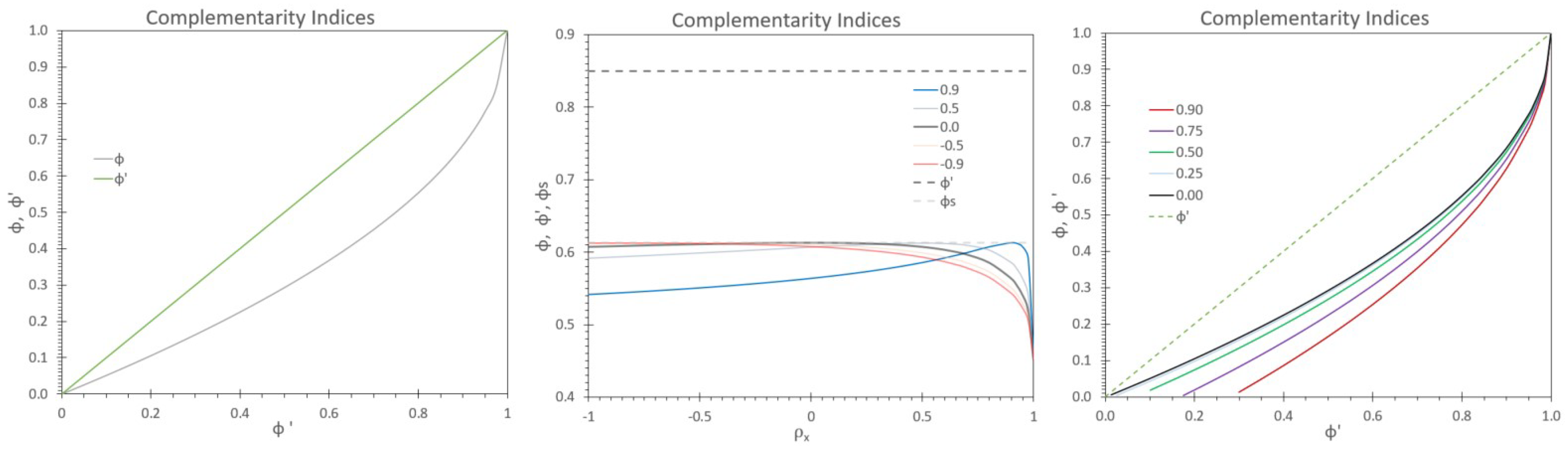
2.2. Total Variation Complementarity Index

Given two functions $f_1\left(t\right)$ and $f_2\left(t\right)$, not both constant, their complementarity index $\varphi (f_1,f_2)$ over the time interval $[a,b]$ is defined as

$$\varphi (f_1,f_2)=1-\frac{{\bigvee }_a^b(f_1+f_2)}{{\bigvee }_a^b\left(f_1\right)+{\bigvee }_a^b\left(f_2\right)}.$$

(5)

Evidently, $0\le \varphi (f_1,f_2)\le 1$, and when $\varphi (f_1,f_2)=1$ a perfect complementarity exists between $f_1$ and $f_2$, and that occurs only if $f_1+f_2$ is a constant. The generalization to any number of functions is direct.

As a special case, consider the Total Variation Complementarity index between the series of anomalies. In weather and climate, an anomaly is the difference of a series compared with its normal or average value. Clearly, the total variation complementarity $\varphi$ between the series $f_1,f_2,\dots ,f_n$, is equal to the complementarity between the series of anomalies with respect to a constant mean for each function

$$\varphi (f_1,f_2,\dots ,f_n)=\varphi (f_1-{\mu }_1,f_2-{\mu }_2,\dots ,f_n-{\mu }_n),$$

(6)

because

$$\frac{{\bigvee }_a^b(f_1+\dots +f_n)}{{\bigvee }_a^b\left(f_1\right)+\dots +{\bigvee }_a^b\left(f_n\right)}=\frac{{\bigvee }_a^b[(f_1-{\mu }_1)+\dots +(f_n-{\mu }_n)]}{{\bigvee }_a^b(f_1-{\mu }_1)+\dots +{\bigvee }_a^b(f_n-{\mu }_n)}.$$

(7)

Summary of the ϕ index characteristics:

• If $f_1$ is the vertical reflection of $f_2$, then $f_1+f_2$ is a constant, therefore, ${\bigvee }_{t_a}^{t_b}(f_1+f_2)=0$ and $\varphi =1$.
• $0\le \varphi \le 1$. For the extreme cases, $\varphi =1$ means that there is perfect complementarity, and for $\varphi =0$ there is no complementarity.
• $\varphi$ is symmetric, this is, $\varphi (f_1,f_2)=\varphi (f_2,f_1)$. Similarly, the symmetry holds for any permutation of the arguments in the case of more than two functions.
• The $\varphi$ index presents the same result when evaluated on anomaly series compared with its corresponding pure series (see Equation (6)).
• The $\varphi$ index could be applied to two or more series.

2.3. Variance Complementarity Index

If one wants to stay within the correlation concept, it is possible to correct the use of $\rho$ as a metric for complementarity to consider the variables’ scale. For that, considering Equation (5), one can replace total variation by variance. This is, given two functions $f_1\left(t\right)$ and $f_2\left(t\right)$, not both constant, their variance complementarity index ${\varphi }_v(f_1,f_2)$ is

$${\varphi }_v(f_1,f_2)=1-\frac{Var[f_1+f_2]}{Var\left[f_1\right]+Var\left[f_2\right]},$$

(8)

which simplifies to

$${\varphi }_v(f_1,f_2)=-\frac{2Cov[f_1,f_2]}{Var\left[f_1\right]+Var\left[f_2\right]}=-{\rho }_{1,2}\frac{2\sqrt{Var\left[f_1\right]Var\left[f_2\right]}}{Var\left[f_1\right]+Var\left[f_2\right]}.$$

(9)

Notice that ${\varphi }_v$ so defined is the negative of the correlation coefficient times the ratio of the geometric and arithmetic means of the variances. This last factor is always less or equal to one, with equality when the two variances are equal. Therefore, ${\varphi }_v(f_1,f_2)$ varies between $-1$ and 1. It is convenient to re-scale it to the range zero to one by means of

$${\varphi }^{\prime }(f_1,f_2)=({\varphi }_v+1)/2.$$

(10)

To illustrate the effect of the scale differences on the complementarity, consider as an example two series with cross-correlation ${\rho }_{1,2}=-0.8$, and the ratio of their standard deviations ${\sigma }_1/{\sigma }_2=5$. Without the correction due to the difference of scales, one overestimates their complementarity, either to be $0.8$ in the range $(-1,1)$ or $0.9$ in the range $(0,1)$. However, considering Equation (9), the complementarities are ${\varphi }_v=0.31$, or ${\varphi }^{\prime }=0.65$. Notice that differences between the means do not play any role. The ratio of the variances is the one that measures the relative scale of the series.

Summary of the ${\varphi }^{\prime }$ index characteristics:

• If $f_1$ is the vertical reflection of $f_2$, $Var\left[f_1\right]=Var\left[f_2\right]$, then ${\rho }_{1,2}=-1$, ${\varphi }_v=1$ and ${\varphi }^{\prime }=1$.
• $0\le {\varphi }^{\prime }\le 1$. For the extreme cases, ${\varphi }^{\prime }=1$ means that there is perfect complementarity, and for ${\varphi }^{\prime }=0$ there is no complementarity.
• ${\varphi }^{\prime }$ is symmetric.
• The ${\varphi }^{\prime }$ index presents the same result when evaluated on anomaly series compared with its corresponding pure series.
• The ${\varphi }^{\prime }$ index could be applied just to two series.

2.4. Standard Deviation Complementarity Index

Using similar reasoning as in Section 2.3, the Standard Deviation Complementarity Index, instead of the variance, measures the variability of the sum with the standard deviation. This way, one stays in the same dimension of the original variables instead of the squares. If $\sigma$ denotes the standard deviation, one can define the index as

$${\varphi }_s(f_1,f_2)=1-\frac{\sigma [f_1+f_2]}{\sigma \left[f_1\right]+\sigma \left[f_2\right]}=1-\sqrt{1-\frac{2\sigma \left[f_1\right]\sigma \left[f_2\right](1-{\rho }_{1,2})}{{(\sigma \left[f_1\right]+\sigma \left[f_2\right])}^2}}.$$

(11)

Recognizing the square of the ratio of the geometric to the arithmetic mean, one can see that ${\varphi }_s$ is in the range $(0,1)$, so there is no need for a re-scaling similar to Equation (10) in the variance index. Moreover, if $\sigma \left[f_1\right]=\sigma \left[f_2\right]$, the equation can be simplified to

$${\varphi }_s(f_1,f_2)=1-\sqrt{\frac{1+{\rho }_{1,2}}{2}}.$$

(12)

The standard deviation complementarity index shares all the corresponding characteristics of ${\varphi }^{\prime }$ listed in the summary above, except number 5.

3. Results

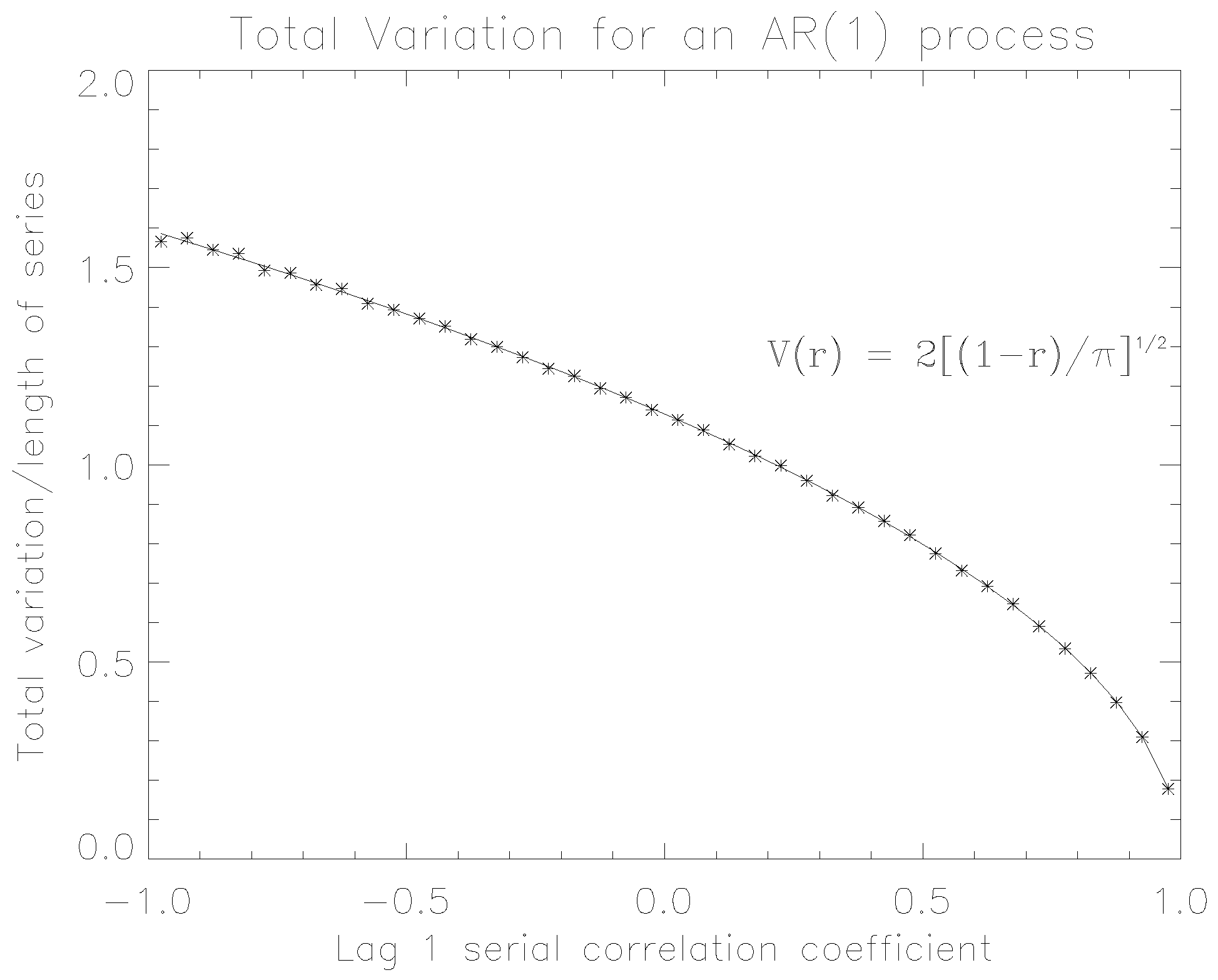
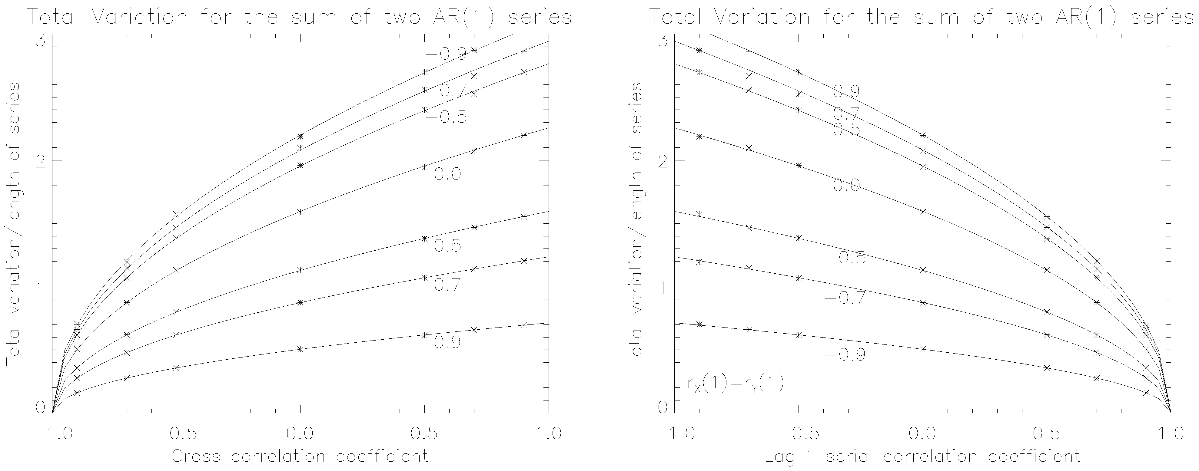
3.1. Case Study 1: Two First-Order Autoregressive Processes

Autoregressive processes are a well-known time series method widely used for all sorts of applications [45]. This section shows an expression for the total variance complementarity index between two cross-correlated autoregressive processes of order one. The purpose is to clarify the two ways of measuring complementarity, namely the total variation and the variance complementarity index.

Let ${\mathbf{z}}_t$ be a vector time series with two components, $x_t$ and $y_t$, both with zero mean and unit variance. The multivariate autoregressive process of order one is

$${\mathbf{z}}_{t+1}={\mathbf{Az}}_t+{\mathbf{Bv}}_{t+1},$$

(13)

where the matrices $\mathbf{A}$ and $\mathbf{B}$ are constant parameters, and ${\mathbf{v}}_t$ is a vector time series of uncorrelated random variables with zero mean and unit variance. This is

$$E\left[{\mathbf{v}}_t\right]=\mathbf{0},Var\left[{\mathbf{v}}_t\right]=E\left[{\mathbf{v}}_t{\mathbf{v}}_t^T\right]=\mathbf{I},Cov[{\mathbf{v}}_t,{\mathbf{v}}_{t+j}]=E\left[{\mathbf{v}}_t{\mathbf{v}}_{t+j}^T\right]=\mathbf{0},$$

for all $j\ne 0$, and $\mathbf{I}$ the identity matrix. For $j>0$, the vector ${\mathbf{v}}_{t+j}$ is uncorrelated with ${\mathbf{z}}_t$,

$$Cov[{\mathbf{z}}_t,{\mathbf{v}}_{t+j}]=E\left[{\mathbf{z}}_t{\mathbf{v}}_{t+j}^T\right]=\mathbf{0}\mathrm{for}j>0.$$

The second order correlation structure of the process ${\mathbf{z}}_t$ depends on the matrices ${\mathbf{M}}_0=Var\left[{\mathbf{z}}_t\right]=E\left[{\mathbf{z}}_t{\mathbf{z}}_t^T\right]$ and ${\mathbf{M}}_1=Cov[{\mathbf{z}}_{t+1},{\mathbf{z}}_t]=E\left[{\mathbf{z}}_{t+1}{\mathbf{z}}_t^T\right]$, with components

$${\mathbf{M}}_0=\left(\begin{array}{cc}Var\left[x_t\right]& Cov[x_t,y_t]\\ Cov[y_t,x_t]& Var\left[y_t\right]\end{array}\right)=\left(\begin{array}{cc}1& {\rho }_{xy}\\ {\rho }_{xy}& 1\end{array}\right),$$

that is symmetric and t-independent, whereas

$${\mathbf{M}}_1=\left(\begin{array}{cc}Cov[x_{t+1},x_t]& Cov[x_{t+1},y_t]\\ Cov[y_{t+1},x_t]& Cov[y_{t+1},y_t]\end{array}\right)=\left(\begin{array}{cc}{\rho }_x& {\rho }_{x_{t+1},y_t}\\ {\rho }_{y_{t+1},x_t}& {\rho }_y\end{array}\right),$$

is not symmetric.

To find expressions for the parametric matrices postmultiply Equation (13) by ${\mathbf{z}}_t$ and take the expected value

$${\mathbf{M}}_{\mathbf{1}}={\mathbf{AM}}_{\mathbf{0}},$$

therefore

$$\mathbf{A}={\mathbf{M}}_{\mathbf{1}}{\mathbf{M}}_{\mathbf{0}}^{-\mathbf{1}}.$$

(14)

Similarly, postmultiply Equation (13) by ${\mathbf{z}}_{t+1}$ and take expected values to obtain

$${\mathbf{M}}_{\mathbf{0}}={\mathbf{M}}_{\mathbf{1}}{\mathbf{M}}_{\mathbf{0}}^{-\mathbf{1}}{\mathbf{M}}_{\mathbf{1}}^{\mathbf{T}}+{\mathbf{BB}}^{\mathbf{T}}.$$

(15)

One can then obtain $\mathbf{B}$ from Equation (15) assuming it is triangular. A simple way is to assume that ${\rho }_{x_{t+1},y_t}={\rho }_{xy}{\rho }_x$ and ${\rho }_{y_{t+1},x_t}={\rho }_{xy}{\rho }_y$ [46]. In that case, ${\mathbf{M}}_{\mathbf{1}}={\mathbf{DM}}_{\mathbf{0}}$, with $\mathbf{D}$ a diagonal matrix

$$\mathbf{D}=\left(\begin{array}{cc}{\rho }_x& 0\\ 0& {\rho }_y\end{array}\right).$$

Therefore, Equation (14) is now

$$\mathbf{A}={\mathbf{M}}_{\mathbf{1}}{\mathbf{M}}_{\mathbf{0}}^{-\mathbf{1}}=\mathbf{D}.$$

(16)

Similarly, Equation (15) simplifies to

$${\mathbf{BB}}^{\mathbf{T}}={\mathbf{M}}_{\mathbf{0}}-{\mathbf{DM}}_{\mathbf{0}}\mathbf{D}=\left(\begin{array}{cc}1-{\rho }_x^2& {\rho }_{xy}(1-{\rho }_x{\rho }_y)\\ {\rho }_{xy}(1-{\rho }_x{\rho }_y)& 1-{\rho }_y^2\end{array}\right),$$

(17)

that one can solve for $\mathbf{B}$

$$\mathbf{B}=\left(\begin{array}{cc}\sqrt{1-{\rho }_x^2}& 0\\ {\displaystyle \frac{{\rho }_{xy}(1-{\rho }_x{\rho }_y)}{\sqrt{1-{\rho }_x^2}}}& \sqrt{1-{\rho }_y^2-{\displaystyle \frac{{\rho }_{xy}^2{(1-{\rho }_x{\rho }_y)}^2}{1-{\rho }_x^2}}}\end{array}\right).$$

(18)

The expected value of the total variation of a univariate autoregressive process (the first component of Equation (13)) is

$$E\left[\underset{1}{\overset{n}{\bigvee }}{x}_t\right]=(n-1)\times {\displaystyle \frac{2}{\sqrt{\pi }}}\sqrt{1-{\rho }_x}.$$

(19)

The Figure 1 shows the expected value as a function of the lag-one autocorrelation coefficient ${\rho }_x$.

The result in Equation (19) comes realizing that

$$|x_{t+1}-x_t|=|\sqrt{1-{\rho }^2}{v}_{t+1}-(1-\rho )x_t|,$$

where both $x_t$ and $v_t$ are independent random variables, with zero mean and unit variance. In addition, one usually assumes that their distribution is Gaussian. Therefore, the expected value of ${\bigvee }_1^n\left(x_t\right)$ is

$$E\left[\underset{1}{\overset{n}{\bigvee }}{x}_t\right]=E\left[\sum _{k=0}^{n-2}|x_{t+1}-x_t|\right]=\sum _{k=0}^{n-2}E\left[|\sqrt{1-{\rho }^2}{v}_{t+1}-(1-\rho )x_t|\right].$$

(20)

A simple calculation of the expected value in Equation (20) gives Equation (19).

Similar arguments apply to the calculation of the expected value of the total variation of the sum $x_t+y_t$

$$E\left[\underset{1}{\overset{n}{\bigvee }}(x_t+y_t)\right]=\sum _{k=0}^{n-2}E\left|(b_{1,1}+b_{2,1})v_{t+1}+b_{2,2}{w}_{t+1}-(1-a_{1,1})x_t-(1-a_{2,2})y_t\right|,$$

(21)

where $a_{i,j}$ and $b_{i,j}$ are, respectively, the components of the matrices $\mathbf{A}$ and $\mathbf{B}$ in Equations (16) and (18). All the random variables in Equation (21) are Gaussian, with zero mean and unit variance. $v_{t+1}$ and $w_{t+1}$ are mutually independent and independent of $x_t$, $y_t$. The covariance between $x_t$ and $y_t$ is ${\rho }_{xy}$. Therefore, using properties of the Gaussian distribution, the absolute value in Equation (21) corresponds to a Gaussian distribution with zero mean and variance equal to

$$\begin{array}{c}\hfill {(b_{1,1}+b_{2,1})}^2+b_{2,2}^2+{(1-a_{1,1})}^2+{(1-a_{2,2})}^2+2(1-a_{1,1})(1-a_{2,2}){\rho }_{xy}=2(1+{\rho }_{xy})(2-{\rho }_x-{\rho }_y).\end{array}$$

Finally, the expected value of the total variation of the sum is

$$E\left[\underset{1}{\overset{n}{\bigvee }}(x_t+y_t)\right]=(n-1)\times {\displaystyle \frac{2}{\sqrt{\pi }}}\sqrt{(1+{\rho }_{xy})(2-{\rho }_x-{\rho }_y)}.$$

(22)

Figure 2 illustrates this result.

Using the above results, Equations (19) and (22), the total variation complementarity index between two autoregressive time series with lag-one correlation coefficients ${\rho }_x$ and ${\rho }_y$, and cross correlation ${\rho }_{xy}$, is

$$\varphi (x_t,y_t)=1-\frac{{\bigvee }_1^n(x_t+y_t)}{{\bigvee }_1^n\left(x_t\right)+{\bigvee }_1^n\left(y_t\right)}=1-{\displaystyle \frac{\sqrt{(1+{\rho }_{xy})(2-{\rho }_x-{\rho }_y)}}{\sqrt{1-{\rho }_x}+\sqrt{1-{\rho }_y}}}.$$

(23)

Figure 3 illustrates some particular cases of this result. We are interested in the comparison of $\varphi$ with ${\varphi }^{\prime }$ and ${\varphi }_s$. Recall that the unit variance of $x_t$ and $y_t$ implies that ${\varphi }^{\prime }(x_t,y_t)=(1-{\rho }_{xy})/2$ and that ${\varphi }_s=1-\sqrt{(1+{\rho }_{xy})/2}$.

A first observation is that for ${\rho }_{xy}=-1$, all three indices $\varphi$, ${\varphi }^{\prime }$, and ${\varphi }_s$ are equal to unity, perfect complementarity regardless of ${\rho }_x$ and of ${\rho }_y$.

Next, if ${\rho }_x={\rho }_y$, the total variation complementarity is independent of ${\rho }_x$, with $\varphi =1-\sqrt{(1+{\rho }_{xy})/2}={\varphi }_s\le {\varphi }^{\prime }=(1-{\rho }_{xy})/2$ (left panel of Figure 3). Interestingly, as functions of ${\rho }_{xy}$, $\varphi$ and ${\varphi }_s$ depend on the square root, whereas ${\varphi }^{\prime }$ is linear. The explanation is that both the definition of the total variance (see Equation (13)) and of the standard deviation are linear on the values of the series, but the cross-correlation is a second-order moment.

Still within the equality of the lag-one correlation coefficients, the case ${\rho }_{xy}=0$, and therefore $\varphi ={\varphi }_s=1-\sqrt{2}/2\approx 0.29$, is interesting in comparison with ${\varphi }^{\prime }=0.5$. That high-variance complementarity index in the absence of cross-correlation comes from how Equation (10) transforms the range of the index between zero and one. Positive cross-correlations give $0<{\varphi }^{\prime }<1/2$, something that seems high. An alternative to Equation (10) could be to take $-{\rho }_{xy}$ for negative correlations and zero for positive ones. However, both are arbitrary. Indeed, one does not need re-scaling for $\varphi$ nor ${\varphi }_s$. For two series with null cross-correlation, approximately 30% of the total variation of their sum cancels out just by chance. In contrast, one of the alternatives of normalizing the variance complementarity to the range $(0,1)$ is too high (50%), and the other is too low (0%). The comment in the previous paragraph has a bearing on this comparison, as the correspondence between $\varphi$ and ${\varphi }_s$ shows.

For constant ${\rho }_{xy}=-0.7$ in the center panel of Figure 3, the total variation complementarity does depend on both ${\rho }_x$ and ${\rho }_y$, although ${\varphi }^{\prime }$ has the constant value of $0.85$. ${\varphi }^{\prime }$ is between 28% and 47% larger than $\varphi$, depending on the values of the autocorrelation coefficients. On the other hand, the comparison between $\varphi$ and ${\varphi }_s$ is better for various values of both ${\rho }_x$ and ${\rho }_y$.

For the case ${\rho }_x=-{\rho }_y$ (right panel of Figure 3), $\varphi$ depends on ${\rho }_x$, except for ${\varphi }^{\prime }$ close to one. In all cases, ${\varphi }^{\prime }$ is larger than $\varphi$. With respect to the comparison between ${\varphi }_s$ and $\varphi$, the first observation is that ${\varphi }_s=\varphi$ for ${\rho }_x=0$. Second, for larger values of the autocorrelation, ${\varphi }_s$ over-estimates $\varphi$, showing the importance of taking into account autocorrelation.

In general, it is worth noticing the contrast between ${\varphi }^{\prime }$ and ${\varphi }_s$ being independent of ${\rho }_x$ and ${\rho }_y$, whereas $\varphi$ is significantly dependent on both.

Recall that all the cases considered in this section use unit variance for the two series to make a fair comparison. Therefore, the possible scale differences do not play a role; only the effect of the serial autocorrelation does.

We conclude that the total variation complementarity index has more information than the variance complementarity or standard deviation indices. It considers the effect of the autocorrelations of the series. In addition, the index based on cross-correlation, ${\varphi }^{\prime }$, significantly overestimates the complementarity compared with $\varphi$. In contrast, for ${\varphi }_s$, the overestimation is less of an issue for a range of autocorrelation values.

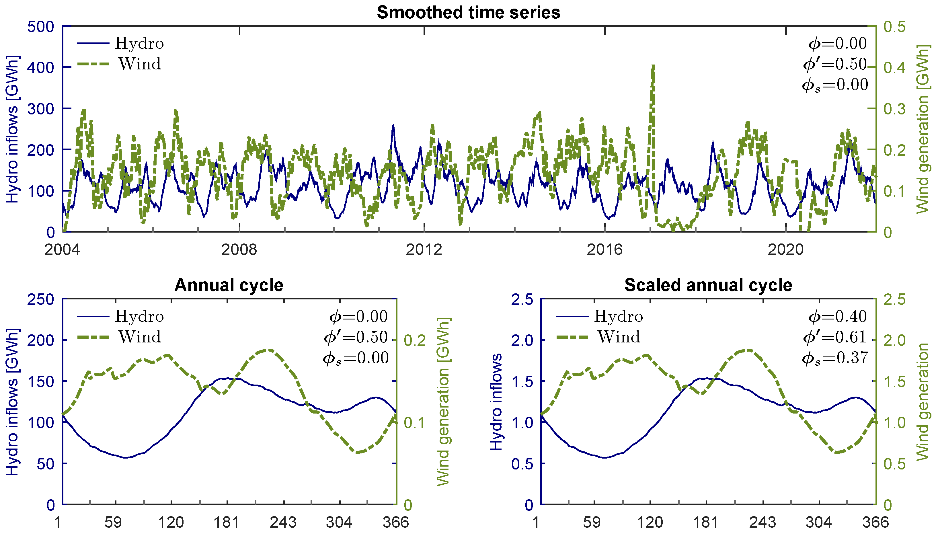
3.2. Case Study 2: Wind vs. Hydro in the Colombian Electricity Market

The total installed capacity for electricity generation in Colombia is approximately 17.5 GW. A total of 68.3% of it comes from hydro sources, while the only wind plant accounts for near 0.1%. This high difference in the scale of both sources has an important impact in the assessment of their complementarity.

To quantify the complementarity between wind and hydro-resources in the Colombian electricity system, we use the daily time series provided by XM, the electric system administrator, and operator in Colombia. For hydro-resources, we analyzed natural inflows (in units of energy) to the main 15 hydropower reservoirs, with a total effective installed capacity of 7668 MW (≈70% of total hydro-capacity) and records from 2000 to 2021. These rivers are San Lorenzo, Nare, Guatapé, San Carlos, Tenche, Guadalupe, Grande, Porce II, Miel I, Urrá, Betania, Batá, Guavio, Alto Anchicayá, and Salvajina. For wind resources, we analyzed daily wind power generation from the Jepirachi plant, with 19.5 MW of effective installed capacity and records for 2004–2021. Notice that the dimensions of both series are the same (energy). The reader can see more details of the hydropower system of Colombia at the XM website (see http://paratec.xm.com.co/paratec/SitePages/Default.aspx, accessed on 30 April 2022).

Figure 4 shows the estimation of $\varphi$, ${\varphi }^{\prime }$, and ${\varphi }_s$ indices to the daily series and the annual cycles of hydro-inflows and wind generation with moving averages of 31 days (top panel). Considering the large-scale difference between the accumulated hydro-inflows and the Jepirachi plant, the scaled series’s complementarity was also studied (bottom panel), with a scale factor of 1/100 for the hydro-inflow series and 1/10 for the wind generation series.

Table 1. Complementarity between daily wind and hydro-resources in Colombia. Both time series were smoothed by a 31-day moving average filter. ${\rho }_1$ represents the exponential value of the slope of the linear regression for the autocorrelation function of both resources.

Group	${\mathit{\sigma }}_{\mathit{H}}^2$ [$\mathit{G}{\mathit{W}}^2{\mathit{h}}^2$]	${\mathit{\rho }}_{1\mathit{H}}$ [-]	${\mathit{\sigma }}_{\mathit{W}}^2$ [$\mathit{G}{\mathit{W}}^2{\mathit{h}}^2$]	${\mathit{\rho }}_{1\mathit{W}}$ [-]	${\mathit{\rho }}_{\mathit{H},\mathit{W}}$ [-]	$\mathit{\varphi }$ [-]	${\mathit{\varphi }}^{\prime }$ [-]	${\mathit{\varphi }}_{\mathit{s}}$ [-]
Smoothed time series	1508	0.98	0.01	0.98	−0.14	0.00	0.50	0.00
Annual cycle	878	-	0.00	-	−0.22	0.00	0.50	0.00
Scaled series	0.09	-	0.13	-	−0.22	0.40	0.61	0.37

presents the results for all analyzed cases.

As expected, because of the two series’ scale differences, the indices $\varphi$, ${\varphi }_v$ (not shown), and ${\varphi }_s$ do not show complementarity. In contrast, the ${\varphi }^{\prime }$ index indicates a complementarity of 0.50 for the daily series and the annual cycle. The reason for this huge overestimation is the way one re-scales the index ${\varphi }_v$ to obtain ${\varphi }^{\prime }$ (Equation (10)).

When using the scaled series, the $\varphi$ index increases to 0.40, and ${\varphi }_s$ to 0.37. We consider that this scaled analysis evaluates the resources’ potential complementarity if the resources’ scales were comparable. There is still a considerable difference in the result of ${\varphi }^{\prime }$. This tendency of ${\varphi }^{\prime }$ to always exceed $\varphi$, overestimating the complementarity quantification, comes from Equation (10).

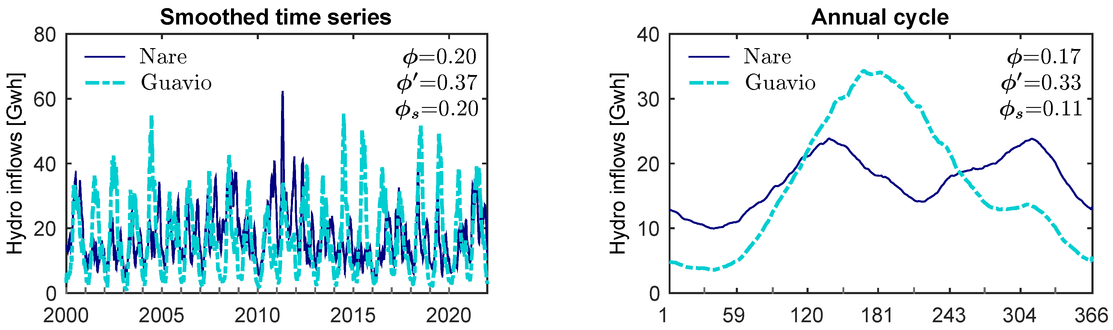
3.3. Case Study 3: Two Hydropower Sources in the Colombian Electricity Market

Nare and Guavio are two important rivers in the hydropower reservoir system of Colombia. According to XM, these rivers belong to different hydrological regions (see details in the XM website: http://portalbissrs.xm.com.co/hdrlg/Paginas/Aportes/apoeneyporreg.aspx, accessed on 30 April 2022). The Andes mountain range separates the two basins, causing significant differences in their hydroclimatic patterns. Seasonality of rainfall is unimodal in the Guavio basin and bimodal in the Nare basin [47]. Streamflows show these regimes, too (Figure 5).

We computed the complementarity indices between the daily natural inflows (in energy units) of the Nare and Guavio rivers for 2000–2021. Figure 5 shows the results, where the left panel shows the 31-day moving average daily inflows and the right panel the annual cycle at daily time-step for both rivers.

Table 2. Complementarity between 31-day moving average daily streamflows of Nare and Guavio rivers. ${\rho }_1$ represents the linear regression slope for the autocorrelation function of both resources.

Group	${\mathit{\sigma }}_{\mathit{N}\mathit{a}\mathit{r}\mathit{e}}^2$ [$\mathit{G}{\mathit{W}}^2{\mathit{h}}^2$]	${\mathit{\rho }}_{1\mathit{N}\mathit{a}\mathit{r}\mathit{e}}$ [-]	${\mathit{\sigma }}_{\mathit{G}\mathit{u}\mathit{a}\mathit{v}\mathit{i}\mathit{o}}^2$ [$\mathit{G}{\mathit{W}}^2{\mathit{h}}^2$]	${\mathit{\rho }}_{1\mathit{G}\mathit{u}\mathit{a}\mathit{v}\mathit{i}\mathit{o}}$ [-]	${\mathit{\rho }}_{\mathit{N}\mathit{a}\mathit{r}\mathit{e},\mathit{G}\mathit{u}\mathit{a}\mathit{v}\mathit{i}\mathit{o}}$ [-]	$\mathit{\varphi }$ [-]	${\mathit{\varphi }}^{\prime }$	${\mathit{\varphi }}_{\mathit{s}}$ [-]
Smoothed time series	62	0.98	129	0.98	0.27	0.20	0.37	0.20
Annual cycle	17	-	101	-	0.50	0.17	0.33	0.11
Scaled series	0.46	-	1.45	-	0.50	0.18	0.29	0.12

lists the results for all analyzed cases.

The scale of both resources is not as different as in the previous case. Consequently, the $\varphi$ index is similar for the daily and scaled series with values close to 0.20. Using the equivalent to Equation (23) that considers the values of variance (not shown), with the parameters contained in Table 2, one gets $\varphi =0.20$. The same value that one obtains using the time series and Equations (4) and (5). This correspondence suggests that the autoregressive model is good for estimating complementarity. Again, ${\varphi }^{\prime }$ shows a higher result than $\varphi$ and ${\varphi }_s$ for all cases, overestimating the complementarity to around 0.38. The pattern is that the variance complementarity index tends to overestimate complementarity.

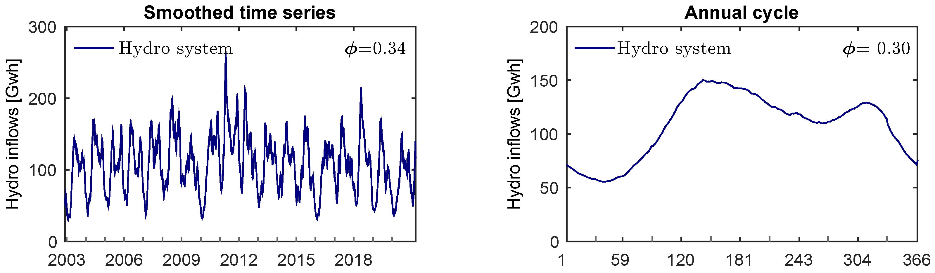
3.4. Case Study 4: Hydropower-Integrated Sources in the Colombian Electricity Market

One of the main advantages of the $\varphi$ index is that one can evaluate the complementarity between any number of series. To illustrate this capability, we quantify the complementarity between the monthly energy inflows to the 15 largest reservoirs of the Colombian hydropower system (described in Section 3.2). This analysis is worthwhile since these reservoirs are in different country regions with different geographic and climatic characteristics.

Figure 6 presents the daily series and annual cycle of the integrated hydro system with moving averages of 31 days. The $\varphi$ index shows a complementarity of 0.34 for the smoothed series and 0.30 for the annual cycles. The complementarity is somewhat higher for the unsmoothed series (not shown), reaching 0.38 and 0.46, respectively.

4. Discussion

This article proposes a novel method based on the concept of Total Variation. The new index ($\varphi$) is a consistent and suitable metric for complementarity between any number of series. The index $\varphi$ measures the regularity of the sum of the variables; this is one minus a measure of irregularity. The new index is not affected by the issues pointed out regarding correlation coefficients. Some essential properties of $\varphi$ are: (1) $\varphi$ is sensitive to the scale of the variables; (2) $\varphi$ works only with dimensionally homogeneous variables; (3) $\varphi$ applies to any number of variables; (4) $\varphi$ also depends on the persistence (autocorrelation) of the series, not only on their cross-correlation.

Given the intermittency of renewable energy sources, consistent evaluation of complementarity is a critical issue. Our proposed index fulfills this need, substantially contributing to energy planning.

The definition of $\varphi$ suggested using the variance instead of total variation to measure irregularity. The result uses the correlation coefficient to assess complementarity. This modification corrects the drawback of differences in the scales of the series discussed above. We call this modification the variance complementarity index, ${\varphi }^{\prime }$. Nevertheless, the correction produces overestimations of complementarity. This overestimation comes from the correlation being a second-order moment. This explanation leads to using the standard deviation instead of the variance to measure the irregularity of the sum. This third index, the Standard Deviation Complementarity Index, corrects the overestimation.

The applications to the Colombian power system show that the variance complementarity overestimates complementarity. In comparison, the Standard Deviation Complementarity Index is closer to the total variation index. However, the analytical results for the expected value of two cross-correlated autoregressive series demonstrate that ${\varphi }_s$ does not capture all the complementarity’s dependencies. In particular, the example shows that serial autocorrelation does affect complementarity.

Finally, we used the proposed indices to quantify the Colombian electricity system’s complementarity. This assessment is important due to its hydrological and climatic regional differences. The total variation complementarity index between the daily series of the hydro-resources is 0.30. This number estimates the complementarity between the 15 main rivers feeding the Colombian power system, which has never been achieved before. The total variation complementarity index, $\varphi$, between hydro and wind resources is almost null due to the wind component’s negligible contribution. When one uses scaled variables, it is 0.39, representing the potential complementarity between these resources and could stimulate a higher level of investment in wind capacity development. The proposed index put a solid basis and a concrete number on those intuitive ideas.

5. Conclusions

There is no agreement in the electricity industry and the scientific community on how to define and assess the complementarity of energy sources. The most frequently used approach is to associate complementarity with negative correlation. This article showed that correlation indices have several intrinsic shortcomings when used for that intention and proposes the uniformity of the sum of the resources as a more physically based concept of complementarity. As a consequence, dimensional homogeneity is a necessary condition for any set of variables before complementarity can be assessed.

There are other drawbacks to the use of correlation coefficients to assess complementarity. (1) If the series scales are very different, correlation coefficients may mislead complementarity. A negative correlation is a necessary but not sufficient condition for complementarity. (2) Correlation coefficients can only be used with pairs of variables, while the applied cases worldwide usually encompass multiple energy sources.

In this article, we propose a new method $\left(\varphi \right)$ based on the concept of Total Variation, which considers as a starting concept to assess complementarity the regularity measure of the sum of the variables. This method is sensitive to the scale of the variables, works only with dimensionally homogeneous variables, depends on the persistence of the series (not only on their cross-correlation), and can be applied to more than two series.

We also present two more indices based on variance $\left({\varphi }^{\prime }\right)$ and standard deviation $\left({\varphi }_s\right)$. We found that the $\left({\varphi }^{\prime }\right)$ index produces complementarity overestimation, on the other hand, although $\left({\varphi }_s\right)$ corrects the overestimation, this index does not capture all the complementarity’s dependencies between the time series.

References

1. Jurasz, J. Modeling and forecasting energy flow between national power grid and a solar–wind–pumped-hydroelectricity (PV–WT–PSH) energy source. Energy Convers. Manag. 2017, 136, 382–394. [Google Scholar] [CrossRef]
2. Moura, P.S.; de Almeida, A.T. Multi-objective optimization of a mixed renewable system with demand-side management. Renew. Sustain. Energy Rev. 2010, 14, 1461–1468. [Google Scholar] [CrossRef]
3. Castro, R.; Crispim, J. Variability and correlation of renewable energy sources in the Portuguese electrical system. Energy Sustain. Dev. 2018, 42, 64–76. [Google Scholar] [CrossRef]
4. Ren, G.; Wan, J.; Liu, J.; Yu, D. Spatial and temporal assessments of complementarity for renewable energy resources in China. Energy 2019, 177, 262–275. [Google Scholar] [CrossRef]
5. Monforti, F.; Huld, T.; Bódis, K.; Vitali, L.; D’Isidoro, M.; Lacal-Arántegui, R. Assessing complementarity of wind and solar resources for energy production in Italy. A Monte Carlo approach. Renew. Energy 2014, 63, 576–586. [Google Scholar] [CrossRef]
6. François, B.; Borga, M.; Anquetin, S.; Creutin, J.; Engeland, K.; Favre, A.C.; Hingray, B.; Ramos, M.; Raynaud, D.; Renard, B.; et al. Integrating hydropower and intermittent climate-related renewable energies: A call for hydrology. Hydrol. Process. 2014, 28, 5465–5468. [Google Scholar] [CrossRef]
7. Slusarewicz, J.H.; Cohan, D.S. Assessing solar and wind complementarity in Texas. Renew. Wind. Water Sol. 2018, 5, 7. [Google Scholar] [CrossRef] [Green Version]
8. Schindler, D.; Behr, H.D.; Jung, C. On the spatiotemporal variability and potential of complementarity of wind and solar resources. Energy Convers. Manag. 2020, 218, 113016. [Google Scholar] [CrossRef]
9. Kay, M. Forecasting and Characterising Grid Connected Solar Energy and Developing Synergies with Wind Project Results and Lessons Learnt; Australian Renewable Energy Agency: Canberra, Australia, 2015; p. 24.
10. Silva, A.R.; Pimenta, F.M.; Assireu, A.T.; Spyrides, M.H.C. Complementarity of Brazil’s hydro and offshore wind power. Renew. Sustain. Energy Rev. 2016, 56, 413–427. [Google Scholar] [CrossRef]
11. de Oliveira Costa Souza Rosa, C.; Costa, K.; da Silva Christo, E.; Braga Bertahone, P. Complementarity of Hydro, Photovoltaic, and Wind Power in Rio de Janeiro State. Sustainability 2017, 9, 1130. [Google Scholar] [CrossRef] [Green Version]
12. dos Anjos, P.S.; da Silva, A.S.A.; Stošić, B.; Stošić, T. Long-term correlations and cross-correlations in wind speed and solar radiation temporal series from Fernando de Noronha Island, Brazil. Phys. A Stat. Mech. Its Appl. 2015, 424, 90–96. [Google Scholar] [CrossRef] [Green Version]
13. Cantão, M.P.; Bessa, M.R.; Bettega, R.; Detzel, D.H.; Lima, J.M. Evaluation of hydro-wind complementarity in the Brazilian territory by means of correlation maps. Renew. Energy 2017, 101, 1215–1225. [Google Scholar] [CrossRef]
14. Xu, L.; Wang, Z.; Liu, Y. The spatial and temporal variation features of wind-sun complementarity in China. Energy Convers. Manag. 2017, 154, 138–148. [Google Scholar] [CrossRef]
15. Li, H.; Liu, P.; Guo, S.; Ming, B.; Cheng, L.; Yang, Z. Long-term complementary operation of a large-scale hydro-photovoltaic hybrid power plant using explicit stochastic optimization. Appl. Energy 2019, 238, 863–875. [Google Scholar] [CrossRef]
16. Cao, Y.; Zhang, Y.; Zhang, H.; Zhang, P. Complementarity assessment of wind-solar energy sources in Shandong province based on NASA. J. Eng. 2019, 2019, 4996–5000. [Google Scholar] [CrossRef]
17. Widen, J. Correlations Between Large-Scale Solar and Wind Power in a Future Scenario for Sweden. IEEE Trans. Sustain. Energy 2011, 2, 177–184. [Google Scholar] [CrossRef]
18. Peña Gallardo, R.; Medina Ríos, A.; Segundo Ramírez, J. Analysis of the solar and wind energetic complementarity in Mexico. J. Clean. Prod. 2020, 268, 122323. [Google Scholar] [CrossRef]
19. Denault, M.; Dupuis, D.; Couture-Cardinal, S. Complementarity of hydro and wind power: Improving the risk profile of energy inflows. Energy Policy 2009, 37, 5376–5384. [Google Scholar] [CrossRef]
20. D’Isidoro, M.; Briganti, G.; Vitali, L.; Righini, G.; Adani, M.; Guarnieri, G.; Moretti, L.; Raliselo, M.; Mahahabisa, M.; Ciancarella, L.; et al. Estimation of solar and wind energy resources over Lesotho and their complementarity by means of WRF yearly simulation at high resolution. Renew. Energy 2020, 158, 114–129. [Google Scholar] [CrossRef]
21. Solomon, A.; Child, M.; Caldera, U.; Breyer, C. Exploiting wind-solar resource complementarity to reduce energy storage need. AIMS Energy 2020, 8, 749–770. [Google Scholar] [CrossRef]
22. Genchi, S.A.; Vitale, A.J.; Piccolo, M.C.; Perillo, G.M. Assessing wind, solar, and wave energy sources in the southwest of Buenos Aires province (Argentina). Investig. Geogr. 2018, 97. [Google Scholar] [CrossRef]
23. Bett, P.E.; Thornton, H.E. The climatological relationships between wind and solar energy supply in Britain. Renew. Energy 2016, 87, 96–110. [Google Scholar] [CrossRef] [Green Version]
24. Sahin, A.Z. Applicability of Wind-Solar Thermal Hybrid Power Systems in the Northeastern Part of the Arabian Peninsula. Energy Sources 2000, 22, 845–850. [Google Scholar] [CrossRef]
25. Odeh, R.P.; Watts, D. Impacts of wind and solar spatial diversification on its market value: A case study of the Chilean electricity market. Renew. Sustain. Energy Rev. 2019, 111, 442–461. [Google Scholar] [CrossRef]
26. Viviescas, C.; Lima, L.; Diuana, F.A.; Vasquez, E.; Ludovique, C.; Silva, G.N.; Huback, V.; Magalar, L.; Szklo, A.; Lucena, A.F.; et al. Contribution of Variable Renewable Energy to increase energy security in Latin America: Complementarity and climate change impacts on wind and solar resources. Renew. Sustain. Energy Rev. 2019, 113, 109232. [Google Scholar] [CrossRef]
27. Gutiérrez, C.; Gaertner, M.Á.; Perpiñán, O.; Gallardo, C.; Sánchez, E. A multi-step scheme for spatial analysis of solar and photovoltaic production variability and complementarity. Sol. Energy 2017, 158, 100–116. [Google Scholar] [CrossRef]
28. Kougias, I.; Szabó, S.; Monforti-Ferrario, F.; Huld, T.; Bódis, K. A methodology for optimization of the complementarity between small-hydropower plants and solar PV systems. Renew. Energy 2016, 87, 1023–1030. [Google Scholar] [CrossRef]
29. Canales, F.A.; Jurasz, J.; Kies, A.; Beluco, A.; Arrieta-Castro, M.; Peralta-Cayón, A. Spatial representation of temporal complementarity between three variable energy sources using correlation coefficients and compromise programming. MethodsX 2020, 7, 100871. [Google Scholar] [CrossRef]
30. Paredes, J.R.; Ramírez, J.J. Variable Renewable Energies and Their Contribution to Energy Security: Complementarity in Colombia. Technical Report; Inter-American Development Bank: Washington, DC, USA, 2017. [Google Scholar]
31. Canales, F.A.; Jurasz, J.; Kies, A.; Beluco, A.; Arrieta-castro, M.; Peralta-cayón, A. Temporal complementarity between three variable renewable energy resources: A spatial representation. In Proceedings of the 11th International Conference on Applied Energy (ICAE), Västerås, Sweden, 12–15 August 2019; pp. 1–6. [Google Scholar]
32. Peña Gallardo, R.; Ospino Castro, A.; Medina Ríos, A. An Image Processing-Based Method to Assess the Monthly Energetic Complementarity of Solar and Wind Energy in Colombia. Energies 2020, 13, 1033. [Google Scholar] [CrossRef] [Green Version]
33. Parra, L.; Gómez, S.; Montoya, C.; Henao, F. Assessing the Complementarities of Colombia’s Renewable Power Plants. Front. Energy Res. 2020, 8. [Google Scholar] [CrossRef]
34. Henao, F.; Viteri, J.P.; Rodríguez, Y.; Gómez, J.; Dyner, I. Annual and interannual complementarities of renewable energy sources in Colombia. Renew. Sustain. Energy Rev. 2020, 134, 110318. [Google Scholar] [CrossRef]
35. Cantor, D.; Ochoa, A.; Mesa, O. Complementariedad hidrológica en Colombia. In Proceedings of the Día de la Energía 2019; Universidad EIA: Envigado, Colombia, 2019. [Google Scholar] [CrossRef]
36. Cantor, D.; Mesa, O.; Ochoa, A. Complementarity beyond correlation. In Complementarity of Variable Renewable Energy Sources; Jurasz, J., Beluco, A., Eds.; Academic Press: London, UK, 2022. [Google Scholar] [CrossRef]
37. Beluco, A.; de Souza, P.K.; Krenzinger, A. A dimensionless index evaluating the time complementarity between solar and hydraulic energies. Renew. Energy 2008, 33, 2157–2165. [Google Scholar] [CrossRef]
38. Borba, E.M.; Brito, R.M. An Index Assessing the Energetic Complementarity in Time between More than Two Energy Resources. Energy Power Eng. 2017, 9, 505–514. [Google Scholar] [CrossRef] [Green Version]
39. Han, S.; Zhang, L.n.; Liu, Y.q.; Zhang, H.; Yan, J.; Li, L.; Lei, X.h.; Wang, X. Quantitative evaluation method for the complementarity of wind–solar–hydro power and optimization of wind–solar ratio. Appl. Energy 2019, 236, 973–984. [Google Scholar] [CrossRef]
40. Neto, P.B.L.; Saavedra, O.R.; Oliveira, D.Q. The effect of complementarity between solar, wind and tidal energy in isolated hybrid microgrids. Renew. Energy 2020, 147, 339–355. [Google Scholar] [CrossRef]
41. Canales, F.A.; Jurasz, J.; Beluco, A.; Kies, A. Assessing temporal complementarity between three variable energy sources through correlation and compromise programming. Energy 2020, 192, 116637. [Google Scholar] [CrossRef] [Green Version]
42. Jurasz, J.; Canales, F.; Kies, A.; Guezgouz, M.; Beluco, A. A review on the complementarity of renewable energy sources: Concept, metrics, application and future research directions. Sol. Energy 2020, 195, 703–724. [Google Scholar] [CrossRef]
43. Kolmogorov, A.; Fomin, S. Introduction Real Analysis; Rev. English, Ed.; Dover: Mineola, NY, USA, 1970. [Google Scholar]
44. Lasota, A.; Mackey, M.C. Chaos, Fractals, and Noise: Stochastic Aspects of Dynamics, 2nd ed.; Springer: New York, NY, USA, 1994. [Google Scholar] [CrossRef]
45. Box, G.E.; Jenkins, G.M.; Reinsel, G.C. Time Series Analysis: Forecasting and Control; John Wiley & Sons: Hoboken, NJ, USA, 2011; Volume 734. [Google Scholar]
46. Matalas, N.C. Mathematical assessment of synthetic hydrology. Water Resour. Res. 1967, 3, 937–945. [Google Scholar] [CrossRef]
47. Urrea, V.; Ochoa, A.; Mesa, O. Seasonality of Rainfall in Colombia. Water Resour. Res. 2019, 55, 4149–4162. [Google Scholar] [CrossRef]
Figure 1. Expected value of the total variation of a univariate autoregressive process as a function of the lag-one autocorrelation coefficient ρ x = r . The points are the average of 100 simulations. The continuous line is Equation (19).
Sustainability 14 08514 g001
Figure 2. Left panel: Expected value of the total variation of the sum of two AR(1) series as a function of the cross-correlation coefficient ρ x y for different values of the serial autocorrelation coefficient ρ y = ρ x , curves are labeled with the respective values of ρ y . Right panel: same as left panel but as a function of ρ y = ρ x for different vales of ρ x y , curves are labeled with the respective values of ρ x y . Points are average of 100 simulations and the continuous line is computed with Equation (22).
Sustainability 14 08514 g002
Figure 3. Comparison of total variation complementarity indices, ϕ , ϕ , and ϕ s as function of ρ x , ρ y and ρ x , y for the sum of two AR(1) series: left panel, when ρ y = ρ x , in this case ϕ = ϕ s ; center panel, when ρ x y = 0.7 , and for the annotated values of ρ y , in this case ϕ = 0.85 and ϕ s = 0.613 ; and right panel, for the annotated values of ρ y = ρ x as a function of ϕ , in this case ϕ s = ϕ for ρ x = 0 .
Sustainability 14 08514 g003
Figure 4. Complementarity indices ϕ , ϕ and ϕ s between wind and hydraulic resources in the Colombia electricity market (time series were smoothed by a 31-day moving average filter). The scale factor in the case of scaled annual cycle is 1/100 for hydro-inflow series and 1/10 for wind-power generation series.
Sustainability 14 08514 g004
Figure 5. Assessment of complementarity by the ϕ , ϕ , and ϕ s indices between the Nare and Guavio rivers. Left panel: 31-day moving average daily inflows. Right panel: annual cycle at daily time-step.
Sustainability 14 08514 g005
Figure 6. Quantification of the complementarity with ϕ index between the energy inflows to the main 15 hydropower reservoirs of the Colombian electricity system, with smoothed moving averages of 31 days.
Sustainability 14 08514 g006